Hyperspectral classification optimization using multiobjective evolutionary algorithm

(1)

HYPERSPECTRAL CLASSIFICATION

OPTIMIZATION USING MULTIOBJECTIVE

EVOLUTIONARY ALGORITHM

CONY SUMORO

B.Eng. (Mechatronics Engineering)

Submitted in fulfilment of the requirements for the degree of

Master of Philosophy

AUSTRALIAN MARITIME COLLEGE

UNIVERSITY OF TASMANIA

(2)

(3)

III

DECLARATION OF ORIGINALITY

This thesis contains no material which has been accepted for a degree or diploma by the University or any other institution, except by way of background information and duly acknowledged in the thesis, and to the best of my knowledge and belief no material previously published or written by another person except where due acknowledgement is made in the text of the thesis, nor does the thesis contain any material that infringes copyrights.

(4)

IV

STATEMENT OF AUTHORITY OF ACCESS

This thesis may be made available for loan and limited copying and communication in accordance with the Copyright Act 1968.

(5)

V

ACKNOWLEDGEMENTS

“HE has made everything beautiful in its time”

– Ecclesiastes 3:11

This thesis would not have been possible without the support of my supervisory team: Hung

Nguyen, Fauzi Hardjanto, and Alex Forrest. I would like to express my sincere thanks to them

for their support and guidance throughout my entire studies.

I could not have completed this thesis without the help from Dr. Christiaan Roelfsema from

University of Queensland and Dr. Hannelie Botha from CSIRO who provide the seagrass

spectral data for research.

Special thanks to the Indonesian community in Launceston especially to Fera who cured my

homesickness with Indonesian food and to Ayu for making jokes to keep me sane. This

endeavour would not be possible without the enormous support from Martin who has been the

light in my life which keeps me motivated when I want to give up. I would like to thank Martin

for bringing balance in my postgraduate studies.

I am very grateful for my parents, Kenny and Irene ,who instil the desire to pursue higher

studies. I am very grateful to them for inspiring me to wander around the world in the pursuit

of knowledge. Last but not least, I would like to thank my brother, William and my sister, Ariel

(6)

VI

ABSTRACT

The development of hyperspectral imagers provides an avenue to exploit it as a bio-optical taxonomic identification tool. In order to classify the species based on their spectral characteristic, spectral similarity measures are usually applied. Five spectral similarity measures are examined: Spectral Correlation Angle (SCA) for calculating the angle of spectral cross-correlation vectors, Spectral Angle Measure (SAM) for the angle between two spectral vectors, Spectral Information Divergence (SID)for measuring the difference in the probability distribution of two spectra, and hybrid measures: SID-SAM and Normalized Spectral Similarity Measure (nSSM). However, currently there is no specific threshold value for each spectral similarity measure that defines positive classification of one specific species. The conventional method by applying either a fixed or an adaptive threshold value is found to be unreliable. The focus of this thesis is to explore the characteristics of different spectral similarity measures and to utilize the MOEA to find the best value for the threshold value. In addition, the research also put forward the parameter test to find the optimum parameter. A machine learning algorithm, SVM is used to compare the performance of MOEA.

(7)

VII

Table of Figures

Figure 1 – Mean ± standard deviation of spectral reflectance of three south-eastern Australian

seagrass species ((Fyfe, 2001) ... 16

Figure 2- (a) Halophia spinulosa (Bryce, 2017), (b) Syringodium isoetifolium (Boisset, 2011), (c) Halophia ovalis (Boisset, 2015), (d)Zostera muelleri (Pocklington, 2011), (e) Cymadosea serrulata (McKenzie, 2007), (f) Halodue univervis(Huisman, 2011) ... 23

Figure 3 – Origin of seagrass sample (Wangawallen banks, west of North Stradbroke island) is circled in red ... 24

Figure 4 - Reflectance spectra of seagrass after smoothing and noise removal ... 25

Figure 5 – Spectra data of terrestrial plants after smoothing and noise removal ... 27

Figure 6 - Flow chart of single objective genetic algorithm ... 28

Figure 7- The flowchart multiobjective GA (NSGA-II) ... 30

Figure 8 - Overview of chromosome initialization ... 32

Figure 9 – Determining false positive and false negative classification ... 34

Figure 10 – Selection in NSGA-II (Deb et al., 2002) ... 35

Figure 11 – Illustration of Non dominated sorting (Zitzler, 1999) ... 36

Figure 12 - Illustration of crowding distance calculation (Deb et al., 2000) ... 37

Figure 13 – Illustration of binary number crossover ... 37

Figure 14 - Probability of expanding and contracting depending on the value of ηc (Agrawal, 1995) 39 Figure 15 – The illustration of the simulated binary crossover with ηc = 20 ... 40

Figure 16- Illustration of binary number mutation ... 40

Figure 16 - The illustration of polynomial mutation ... 41

Figure 18 - The population in decision space (a) before NSGA-II, (b) after running 100th_{generation 42} Figure 18 - Illustration of the distance measurement ... 42

Figure 20 – Effects of different number of generation to misclassification rate (seagrass) ... 47

Figure 21 - Effects of different number of generation to misclassification rate (terrestrial plants) ... 48

Figure 22 - (a) normal probability plot of residuals and (b) residuals versus fitted values – Cymadocea serrulata ... 49

Figure 23 – Contour plot of misclassification rate – Cymadocea serrulata ... 50

Figure 24 – (a) normal probability plot of residuals and (b) residuals versus fitted values – Halodue univervis ... 51

Figure 25 - Contour plot of misclassification rate – Halodue univervis ... 51

Figure 26 – (a) normal probability plot of residuals and (b) residuals versus fitted values – Halophia ovalis ... 52

Figure 27 - Contour plot of misclassification rate – Halophia ovalis ... 53

Figure 28 – (a) Normal probability plot for residuals and (b) residuals versus fitted value – Halophia spinulosa ... 54

Figure 29 - Contour plot of misclassification rate – Halophia spinulosa ... 54

Figure 30- (a) normal probability plot of residuals and (b) residuals versus fitted values – Syringodium isoetofolium ... 55

Figure 31 – Contour plot of misclassification rate – Syringodium isoetofolium ... 56

Figure 32- (a) normal probability plot of residuals and (b) residuals versus fitted values – Zostera muelleri ... 57

Figure 33 – (a) Response surface and (b) contour plot of misclassification rate – Zostera muelleri .... 57

Figure 34- (a) normal probability plot of residuals and (b) residuals versus fitted values – Eucalyptus ... 58

(10)

X

Figure 36 - (a) normal probability plot of residuals and (b) residuals versus fitted values – Blackberry

... 60

Figure 37 - Contour plot of misclassification rate – Blackberry ... 60

Figure 38 - (a) normal probability plot of residuals and (b) residuals versus fitted values – Lemon ... 61

Figure 39 – (a) Response surface and (b) contour plot of misclassification rate – Lemon ... 62

Figure 40 - (a) normal probability plot of residuals and (b) residuals versus fitted values – Cherry plum ... 63

Figure 41 - Contour plot of misclassification rate – Cherry plum ... 63

Figure 42 - Comparison of misclassification rate among spectral similarity measures for seagrass .... 66

Figure 43 - Average misclassification rate among seagrasses for different methods ... 67

Figure 44 - Comparison of misclassification rate among spectral similarity measures for terrestrial plants ... 68

Figure 45 - Average misclassification rate among terrestrial plants for different methods ... 69

Figure 46 - PSD for different spectral measures applied to different type of seagrass ... 70

Figure 47 – PSD statistics for different similarity measures on terrestrial plants ... 71

Figure 48 –PWSD of different spectral similarity measures applied to (a) Cymadocea serrulata, (b) Halodue univervis, (c) Halophia ovalis, (d) Halophia spinulosa, (e) Syringodium isoetofolium, and (f) Zostera muelleri ... 72

(11)

XI

Table of Tables

Table 1- Matrix for false positive and false negative classification ... 33

Table 2 - Example of non-dominated sorting ... 36

Table 3 – Parameters for unoptimized MOEA ... 43

Table 4 – Result of 3-way ANOVA – Cymadocea serrulata ... 49

Table 5 – Result of 3-way ANOVA – Halodue univervis ... 50

Table 6 - Result of 3-way ANOVA – Halophia ovalis ... 52

Table 7- Result of 3-way ANOVA – Halophia spinulosa... 53

Table 8 - Result of 3-way ANOVA – Syringodium isoetofolium ... 55

Table 9 - Result of 3-way ANOVA – Zostera muelleri ... 56

Table 10 - Result of 3-way ANOVA – Eucalyptus... 58

Table 11- Result of 3-way ANOVA – Blackberry... 59

Table 12- Result of 3-way ANOVA – Lemon ... 61

Table 13 - Result of 3-way ANOVA – Cherry plum ... 62

Table 14 - List of the optimum parameters ... 64

(12)

XII

Nomenclatures

ri and si Spectral vectors

Relative entropy of 𝑠𝑠_𝑖𝑖 relative to 𝑟𝑟_𝑖𝑖 Relative entropy of 𝑟𝑟_𝑖𝑖 relative to 𝑠𝑠_𝑖𝑖 Self-information measure for ri

Self-information measure for 𝑠𝑠_𝑖𝑖 Probability vector p

Probability vector q

LU Upwelling radiance

Ed Downwelling irradiance

False positive rate Number of false positive Number of positive sample False negative rate

Number of false negative Number of negative sample Total probability of false negative Total probability of false positive Crowded comparison

Nondomination rank Crowding distance

Fi Front i

𝑖𝑖𝑡𝑡ℎ_{child with}_𝑘𝑘𝑡𝑡ℎ_{component (crossover)} 𝑖𝑖𝑡𝑡ℎ_{parent with}_𝑘𝑘𝑡𝑡ℎ_{component (crossover)} Random number

Crossover distribution index

Child with 𝑘𝑘𝑡𝑡ℎ component (mutation) Parent with 𝑘𝑘𝑡𝑡ℎ component (mutation) Upper bound of the parent

(13)

XIII Distance of ith_chromosome

xi Distance to the point on x-axis

yi Distance to the point on y-axis

(14)

XIV

Abbreviations

ANOVA Analysis of Variance

BB Blackberry

BLX-a Blend Crossover

CP Cherry Plum

CS Cymadocea Serrulata

EU Eucalyptus

FCB Fuzzy Connective Based

FR Fuzzy Recombination

GA Genetic Algorithm

HO Halophia ovalis

HS Halophia spinulosa

HU Halodue univervis

LM Lemon

MOEA Multiobjective Evolutionary Algorithm

NSGA Nondominated Sorting Genetic Algorithm

NSGA-II Nondominated Sorting Genetic Algorithm - II

nSSM Normalized Spectral Similarity Measure

PSD Probability of Spectral Discrimination

PWSD Power of Spectral Discrimination

SAM Spectral Angle Mapper

SBX Simulated Binary Crossover

SCA Spectral Correlation Angle

SCM Spectral Correlation Measure

SI Syringodium isoetofolium

SID Spectral Infromation Divergence

SID-SAM Spectral Infromation Divergence - Spectral Angle Mapper

VEGA Vector Evaluated Genetic Algorithm

VNIR Visible Near Infrared

(15)

15

Chapter 1 Introduction

"A trick is nothing but a puzzle mankind came up with. If you use your head, you can uncover the

logical answer."

Shinichi Kudo

1.1 Background

Periodic survey to identify plant in an ecosystem is important to monitor the health of ecosystem, which is measured by the change in the composition of species, for example, in the coastal environment (Rosenberg et al., 2004). Other than monitoring the health of the ecosystem, plant identification is also beneficial to early detection of the introduction of invasive species, such as Undaria pinnatifida or Wakame seaweed which was introduced by hull fouling to Australian coastal water (Hewitt et al., 1999).

(16)

16

continuous spectral information in a hyperspectral image allow for identification of different materials based on their spectral characteristics.

Hyperspectral imagers have been used in different areas of remote sensing application, such as geology (van der Meer, 2006), agriculture (Aasen et al., 2014), vegetation (Du et al., 2004) for decades. Reflectance spectra obtained from underwater hyperspectral imaging have been used as bio-taxonomic identification of corals (Kutser and Jupp, 2006, Botha et al., 2013), micro- and microalgae (Volent et al., 2009, Kutser and Metsamaa, 2006) and seagrass (Fyfe, 2001, Paringit et al., 2003). Fyfe (2001) sampled the spectral reflectance of three different seagrass species and found distinct spectral signatures of Zostera capricorni, Halophia ovalis, and Posidonia australis as shown in Figure 1. At 675 nm wavelength, Z.capricorni and P. Australis absorbed more light than H. Ovalis. Compared to the rest, Z. capricorni lacks intense green reflectance at 550 nm wavelength. The largest difference in the spectral

reflectance of the three species takes place at the Near Infra-Red (NIR) region (700nm – 900 nm).

Figure 1 – Mean ± standard deviation of spectral reflectance of three south-eastern Australian seagrass species ((Fyfe,

2001)

1.2 Quantification of Spectral Information and Species Identification

(17)

17

methods in hyperspectral classification due to its simplicity as it does not require complex analysis and dimension reduction(Ma et al., 2016). The accuracy of the spectral similarity measure depends on its discrimination threshold, which varies for different material or biological species. The use of spectral similarity measure to classify a target species is carried out by the comparison of the spectra from the target species with the reference spectra in a spectral library. The measure assumes that the target is of a particular species if the similarity measure of target spectra and reference spectra of that particular species in the library is under certain discrimination threshold.

To date, no specific way has been identified to ascertain the definitive threshold value for discriminating terrestrial and underwater plants. The conventional way in remote sensing of minerals is to apply a user-defined or fixed value on a specific spectral similarity measure, such as 0.1 for Spectral Angle Mapper (SAM) (Shahriari et al., 2014). However, the conventional fixed threshold value does not necessarily provide a high capability to discriminate plants. Schwarz and Staenz (2001) introduced an adaptive threshold on the assumption of Gaussian distribution of the spectral angles. They concluded that the threshold value might be given by the mean minus three standard deviation. Shahriari et al. (2014) generalized this idea and proposed that the threshold value might be given by the mean minus m times the standard deviation, where m is a value ranging from one to three. The adaptive method shows better identification compared to the use of typical fixed value or user-defined method.

An optimum threshold determination is defined by the minimization of the probability of both false-positive and false-negative identification of species. False false-positive, also known as “false alarm”, refers to a similarity detection of otherwise dissimilar species. False negative, or “missed detection”, refers to similar species being recognized differently. A minimization problem of this type constitutes a multiobjective optimization which can be solved using the multiobjective variant of genetic algorithm.

1.3 Machine Learning Classifier

(18)

18

infinite dimensional space, which gives the largest separation distance among the training data point. Since in principle, the larger separation distance the lower misclassification, SVM is a robust classification method. It has already been applied in the hyperspectral classification problem such as hyperspectral remote sensing classification (Gualtieri and Cromp, 1999), and underwater benthic classification (Bongiorno, 2014). Being considered as the state of art method of classification, SVM is used as a comparison benchmark in this thesis.

1.4 Research Aim and Objectives

The research in this thesis aims to optimize the classification of plant species using five different spectral similarity measures, namely Spectral Angle Mapper (SAM), Spectral Correlation Angle (SCA), Spectral Information Divergence (SID), SID-SAM and Normalized Spectral Similarity Measure (nSSM). As previously mentioned, the accurate classification requires the minimization of both false positive and false negative identification. The novel aspect of this research is about the formulation and the application of the Multiobjective Evolutionary Algorithm (MOEA), which is based on the genetic algorithm, to find the optimal threshold value of each of the five spectral similarity measures in identifying different seagrass and terrestrial species. Additionally, parameters contributing to the MOEA performance are also quantified. It is expected that the optimized threshold leads to more robust classification of seagrasses and terrestrial species using hyperspectral information.

1.5 Thesis Structure

(19)

19

Chapter 3 discusses the results of the MOEA algorithm to determine the optimum threshold value for each spectral similarity measure. It is followed by a comparison of the misclassification rate from the adaptive threshold method, SVM, MOEA with fixed parameters, and MOEA with optimized parameters.

(20)

20

Chapter 2 Methods

"Although this mirror can show a reflection, it cannot show you the truth."

Ai Haibara

2.1 Spectral Similarity Measures

The formulation of spectral similarity measures can be categorized as follows:

1. Deterministic, which includes Spectral Angle Mapper (SAM), Spectral Correlation Angle (SCA) and Normalized Spectral Similarity Measure (nSSM);

2. Stochastic, which includes Spectral Information Divergence (SID); and 3. Hybrid, such as SID-SAM.

The following sub-sections present a description of each measure:

2.1.1 Spectral Correlation Angle (SCA)

Van Der Meer and Bakker (1997) proposed a spectral correlation measure (SCM) of two spectral vectors, 𝑟𝑟_𝑖𝑖 and𝑠𝑠_𝑖𝑖, be given as a function of the Pearson’s cross correlation (Pearson, 1901) given by:

𝑆𝑆𝑆𝑆𝑆𝑆= 𝑛𝑛 ∑𝑛𝑛𝑖𝑖=1𝑟𝑟𝑖𝑖𝑖𝑖𝑠𝑠𝑖𝑖𝑖𝑖− ∑𝑛𝑛𝑖𝑖=1𝑟𝑟𝑖𝑖𝑖𝑖∑𝑛𝑛𝑖𝑖=1𝑠𝑠𝑖𝑖𝑖𝑖

�[𝑛𝑛 ∑𝑖𝑖=1𝑛𝑛 𝑟𝑟𝑖𝑖𝑖𝑖2−(∑𝑛𝑛𝑖𝑖=1𝑟𝑟𝑖𝑖𝑖𝑖)2][𝑛𝑛 ∑ 𝑠𝑠𝑖𝑖𝑖𝑖𝑛𝑛1 2−(∑𝑛𝑛𝑖𝑖=1𝑠𝑠𝑖𝑖𝑖𝑖)2]

(1)

where i is the index of wavelength, and n is the number of spectral bands. Bajwa et al. (2004) then converted the correlation measure to angle measure which is shown as follows:

𝑆𝑆𝑆𝑆𝑆𝑆�𝑠𝑠𝑖𝑖,𝑠𝑠𝑗𝑗�= 𝑐𝑐𝑐𝑐𝑠𝑠−1 �𝑆𝑆𝑆𝑆𝑆𝑆₂+ 1� (2)

(21)

21

allows the matching of different albedo; however, a small shift in the position of the absorption band and shape on the spectral vector affects the SCA value. The two spectra are considered as similar if the SCA is zero and dissimilar if SCA is 1.57.

2.1.2 Spectral Angle Mapper (SAM)

Spectral angle mapper measures the angle of the dot product of two spectral vectors 𝑟𝑟_𝑖𝑖 and 𝑠𝑠_𝑖𝑖:

𝑆𝑆𝑆𝑆𝑆𝑆(𝑟𝑟𝑖𝑖,𝑠𝑠𝑖𝑖) =𝑐𝑐𝑐𝑐𝑠𝑠−1 ⎝

⎛ ∑𝑛𝑛𝑖𝑖=1𝑟𝑟𝑖𝑖𝑖𝑖𝑠𝑠𝑖𝑖𝑖𝑖 �∑𝑛𝑛 𝑟𝑟_{𝑖𝑖𝑖𝑖}2

𝑖𝑖=1 �∑𝑛𝑛𝑖𝑖=1𝑠𝑠𝑖𝑖𝑖𝑖2_⎠

⎞ (3)

where i is the index of wavelength, and n is the number of bands. Similar to SCA, SAM is relatively insensitive to different brightness since the angle between two spectra vectors is independent from the length or magnitude of the vectors. The SAM goes from 0 when the spectra signatures are identical to 1.57 when they are completely different.

2.1.3 Normalized Spectral Similarity Measure (nSSM)

One of the most widely used metrics to measure the difference in albedo variation given by the spectral magnitude is the Euclidian distance (ED) (Keshava, 2004). Botha et al. (2013) introduced a Normalized Spectral Similarity Measures (nSSM) which combines the SAM that measures the difference in the spectral shape and a normalized Euclidian distance (NED) which accounts for the albedo variation. The nSSM is defined as:

𝑛𝑛𝑆𝑆𝑆𝑆𝑆𝑆 = �𝑆𝑆𝑆𝑆𝑆𝑆2₊_{𝑁𝑁𝑁𝑁𝑁𝑁}2 (4)

where SAM is given in Eq. (3) and NED of the spectral signatures, 𝑟𝑟_𝑖𝑖 and 𝑠𝑠_𝑖𝑖 is given as:

𝑁𝑁𝑁𝑁𝑁𝑁= �∑_∑𝑛𝑛𝑖𝑖=1(𝑟𝑟𝑖𝑖𝑖𝑖 − 𝑠𝑠𝑖𝑖𝑖𝑖)2 (𝑟𝑟𝑖𝑖𝑖𝑖 +𝑠𝑠𝑖𝑖𝑖𝑖)2 𝑛𝑛

𝑖𝑖=1

(5)

(22)

22

2.1.4 Spectral Information Divergence (SID)

Spectral information divergence is a stochastic measure which calculates the difference in the probability distribution of two spectra (Chang, 2003). The SID between two spectral signatures 𝑟𝑟_𝑖𝑖 and 𝑠𝑠𝑖𝑖 is defined as:

𝑆𝑆𝑆𝑆𝑁𝑁(𝑟𝑟𝑖𝑖,𝑠𝑠𝑖𝑖) =𝑁𝑁(𝑟𝑟𝑖𝑖||𝑠𝑠𝑖𝑖) +𝑁𝑁(𝑠𝑠𝑖𝑖||𝑟𝑟𝑖𝑖) (6) where,

𝑁𝑁(𝑟𝑟𝑖𝑖||𝑠𝑠𝑖𝑖) = � 𝑞𝑞𝑖𝑖�𝑆𝑆𝑖𝑖(𝑠𝑠𝑖𝑖)− 𝑆𝑆𝑖𝑖(𝑟𝑟𝑖𝑖)� 𝑛𝑛

𝑖𝑖=1

(7) and

𝑁𝑁(𝑠𝑠𝑖𝑖||𝑟𝑟𝑖𝑖) = � 𝑝𝑝𝑖𝑖�𝑆𝑆𝑖𝑖(𝑟𝑟𝑖𝑖)− 𝑆𝑆𝑖𝑖(𝑠𝑠𝑖𝑖)� 𝑛𝑛

𝑖𝑖=1

(8)

where i is the index of wavelength, and n is the number of spectral bands. 𝑁𝑁(𝑟𝑟_𝑖𝑖||𝑠𝑠_𝑖𝑖) and 𝑁𝑁(𝑠𝑠_𝑖𝑖||𝑟𝑟_𝑖𝑖) are called the relative entropy of 𝑠𝑠_𝑖𝑖 relative to 𝑟𝑟_𝑖𝑖 and the relative entropy of 𝑟𝑟_𝑖𝑖 relative to 𝑠𝑠_𝑖𝑖, respectively. The probability vector 𝑝𝑝= (𝑝𝑝1,𝑝𝑝2, … ,𝑝𝑝𝑖𝑖) and 𝑞𝑞= (𝑞𝑞1,𝑞𝑞2, … ,𝑞𝑞𝑖𝑖) are given as 𝑝𝑝𝑛𝑛=𝑠𝑠𝑖𝑖𝑖𝑖/∑𝑛𝑛_𝑖𝑖=1𝑠𝑠𝑖𝑖𝑖𝑖 and 𝑞𝑞𝑛𝑛=𝑠𝑠𝑗𝑗𝑖𝑖/∑𝑛𝑛𝑖𝑖=1𝑠𝑠𝑗𝑗𝑖𝑖. 𝑆𝑆𝑖𝑖(𝑟𝑟𝑖𝑖𝑖𝑖) and 𝑆𝑆𝑖𝑖(𝑠𝑠𝑖𝑖𝑖𝑖) are values of self-information measures given by 𝑆𝑆𝑖𝑖(𝑟𝑟𝑖𝑖𝑖𝑖) =

−log𝑞𝑞𝑖𝑖 and 𝑆𝑆𝑖𝑖(𝑠𝑠𝑖𝑖𝑖𝑖) = −log𝑝𝑝𝑖𝑖, respectively.

The value of SID is equal to zero when the two spectral vectors are perfectly identical, and SID reaches infinity when the two spectral vectors are totally different.

2.1.5 SID-SAM

This hybrid method was first introduced by Du et al. (2004). It increases discriminability by making two similar spectra more similar and two different spectra more distinctive. There are two versions of this technique:

SID-SAM(TAN) = SID(𝑟𝑟_𝑖𝑖,𝑠𝑠𝑖𝑖). tan�SAM(𝑟𝑟_𝑖𝑖,𝑠𝑠𝑖𝑖)� (9) and

(23)

23

where 𝑟𝑟𝑖𝑖 and 𝑠𝑠𝑖𝑖 are the spectral signatures. The value of SID-SAM is equal to zero when the two spectral vectors are completely similar and infinity when the two spectral vectors are entirely distinct.

2.2 Spectral Data

2.2.1 Seagrass Samples

In principle, the purest spectra are those that are measured in-situ. However, measuring spectra reflectance underwater has several challenges due to limited light underwater and equipment capabilities, and since the scope of this thesis is only focusing on the classification. Therefore, the seagrass samples are only of those taken in air.

Seagrass samples examined in this thesis are Halophia spinulosa (Figure 2a), Syringodium isoetifolium (Figure 2b), Halophia ovalis (Figure 2c), Zostera muelleri (Figure 2d), Halodue univervis (Figure 2e), and Cymadocea serrulata (Figure 2f).

(a) (b) (c)

(d) (e) (f)

Figure 2- (a) Halophia spinulosa (Bryce, 2017), (b) Syringodium isoetifolium (Boisset, 2011), (c) Halophia ovalis (Boisset,

2015), (d)Zostera muelleri (Pocklington, 2011), (e) Cymadosea serrulata (McKenzie, 2007), (f) Halodue univervis(Huisman,

[image:23.595.73.522.393.702.2]

(24)

24

The spectral data of each sample is obtained from Roelfsema et al. (2016). They measured the reflectance spectra for wavelengths between 400 and 1050 nm in 1024 bands using ASD VNIR spectrometer. To account for the upwelling radiance (LU) under the sunlight at the location of the

measurement, the spectrometer optics was placed 15 cm above the target. To estimate the downwelling irradiance, the reflectance of a spectralonTM_{panel, which is assumed to be 100% Lambertian surface,}

[image:24.595.186.411.281.644.2]

was measured at the same location within the same time period. The six types of seagrass species from different individuals were collected and measured on 16th January 2001 between 3 to 5 pm at Wangawallen banks, West North Stradbroke Island in Moreton Bay, Queensland (Figure 3).

Figure 3 – Origin of seagrass sample (Wangawallen banks, west of North Stradbroke island) is circled in red

(25)

25

[image:25.595.76.528.127.697.2]

the six different types of seagrass. The radiance-reflectance signature was obtained by dividing the measured reflectance by the radiance reflected by the Spectralon (LU/Ed).

Figure 4 - Reflectance spectra of seagrass after smoothing and noise removal

(26)

26

the signal and lead to lower correlation between spectral vectors. Figure 4 above shows the reflectance spectra after smoothing and removal of the noise.

The ten spectral data for each species are divided randomly into two sets: five spectra for training set and five spectra for evaluation set. The training set used for optimization purposes and the evaluation set is used to assess the performance of the optimized parameters of MOEA.

2.2.2 Terrestrial Plant Samples

Collection of spectral data of four species of terrestrial plants was carried out by the author of this thesis. The four species include Eucalyptus (Eucalyptus globulus), Lemon (Citrus limon), Blackberry (Rubus fruticosus agg.), and Cherry plum (Prunus cerasifera). The measurement was performed using Ocean Optics STS-VIS spectrometer which measures the reflectance between 350 – 800 nm. The data acquisition was taken indoor using the OCEANVIEW program with Ocean Optics ECO-VIS light as light source and Spectralon as reference. Other source of light indoor was minimized during measurement to prevent interference on the reflectance.

(27)

27

Figure 5 – Spectra data of terrestrial plants after smoothing and noise removal

2.3 Genetic Algorithm

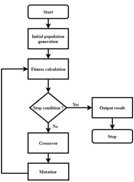
Genetic algorithm (GA) is a directed random search algorithm that is inspired by natural evolution selection and genetics (Goldberg, 1988). It is, therefore, suited for applications in optimization or machine learning problems. Genetic algorithm was developed by John Holland and his collaborators at the University of Michigan (Holland, 1975).

The idea of GA is to evolve the population of solutions using operators, i.e. crossover and mutation which are based on the mechanics of natural selection and genetic variation. The crossover is the swapping of the parents’ solutions (genes) to produce different offspring. Mutation is the mutating one solution (gene) in the parent chromosome to produce a different offspring. These operators aim to improve the fitness of the chromosomes over the generations. The fitness is defined as the closeness of the solutions to the optimum. The individuals that provide better solution (fitness) have greater probability to be preserved and reproduced in the next generation (Davis, 1991). The algorithm efficiently exploits the fitness evaluation of previous solution to predict a new solution with the expectation for an improved accuracy.

(28)

[image:28.595.162.434.68.437.2]

28

Figure 6 - Flow chart of single objective genetic algorithm

(29)

29

The multi-objective evolutionary algorithm (MOEA), on the other hand, tries to determine a set of pareto optimal solutions. Pareto optimal solutions offer the best trade-off among the objectives. This approach is considered more robust than the preference based approaches since a large optimization search space can be handled and multiple alternative trade-offs can be generated within a single run (Zitzler, 1999, Deb et al., 2002).

2.4 Multiobjective Evolutionary Algorithm

(30)

30

[image:30.595.128.474.64.621.2]

(31)

31

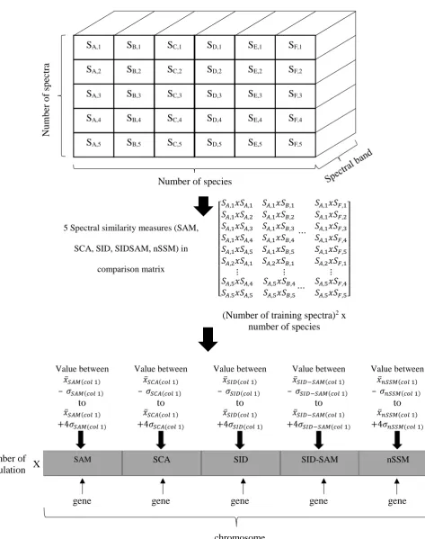
2.5 Initialization

The first step in applying the MOEA is the initialization of chromosomes. A chromosome is a set of parameters that define the proposed solutions to the problem. Instead of randomly generated numbers to initialize chromosome, this research uses the spectral similarity measures from the spectra to obtain guided chromosome values.

(32)

32

5 Spectral similarity measures (SAM,

SCA, SID, SIDSAM, nSSM) in

comparison matrix ⎣ ⎢ ⎢ ⎢ ⎢ ⎢ ⎢ ⎢ ⎢

⎡𝑆𝑆_𝑆𝑆𝐴𝐴,1𝑥𝑥𝑆𝑆𝐴𝐴,1

𝐴𝐴,1𝑥𝑥𝑆𝑆𝐴𝐴,2

𝑆𝑆𝐴𝐴,1𝑥𝑥𝑆𝑆𝐴𝐴,3

𝑆𝑆𝐴𝐴,1𝑥𝑥𝑆𝑆𝐵𝐵,1

⋯

𝑆𝑆𝐴𝐴,1𝑥𝑥𝑆𝑆𝐹𝐹,1

⋮ ⋮ ⋮

𝑆𝑆𝐴𝐴.5𝑥𝑥𝑆𝑆𝐴𝐴,5

𝑆𝑆𝐴𝐴,5𝑥𝑥𝑆𝑆𝐵𝐵,5⋯

𝑆𝑆𝐴𝐴,5𝑥𝑥𝑆𝑆𝐹𝐹,5⎦

⎥ ⎥ ⎥ ⎥ ⎥ ⎥ ⎥ ⎥ ⎤

(Number of training spectra)2_x

number of species

Value between

𝑥𝑥̅𝑆𝑆𝐴𝐴𝑆𝑆(𝑐𝑐𝑐𝑐𝑖𝑖1)

– 𝜎𝜎𝑆𝑆𝐴𝐴𝑆𝑆(𝑐𝑐𝑐𝑐𝑖𝑖1)

to 𝑥𝑥̅𝑆𝑆𝐴𝐴𝑆𝑆(𝑐𝑐𝑐𝑐𝑖𝑖1)

+4𝜎𝜎𝑆𝑆𝐴𝐴𝑆𝑆(𝑐𝑐𝑐𝑐𝑖𝑖1)

Value between

𝑥𝑥̅𝑆𝑆𝑆𝑆𝐴𝐴(𝑐𝑐𝑐𝑐𝑖𝑖1)

– 𝜎𝜎𝑆𝑆𝑆𝑆𝐴𝐴(𝑐𝑐𝑐𝑐𝑖𝑖1)

to 𝑥𝑥̅𝑆𝑆𝑆𝑆𝐴𝐴(𝑐𝑐𝑐𝑐𝑖𝑖1)

+4𝜎𝜎𝑆𝑆𝑆𝑆𝐴𝐴(𝑐𝑐𝑐𝑐𝑖𝑖1)

Value between

𝑥𝑥̅𝑆𝑆𝑆𝑆𝑆𝑆(𝑐𝑐𝑐𝑐𝑖𝑖1)

– 𝜎𝜎𝑆𝑆𝑆𝑆𝑆𝑆(𝑐𝑐𝑐𝑐𝑖𝑖1)

to 𝑥𝑥̅𝑆𝑆𝑆𝑆𝑆𝑆(𝑐𝑐𝑐𝑐𝑖𝑖1)

+4𝜎𝜎𝑆𝑆𝑆𝑆𝑆𝑆(𝑐𝑐𝑐𝑐𝑖𝑖1)

Value between

𝑥𝑥̅𝑆𝑆𝑆𝑆𝑆𝑆−𝑆𝑆𝐴𝐴𝑆𝑆(𝑐𝑐𝑐𝑐𝑖𝑖1)

– 𝜎𝜎𝑆𝑆𝑆𝑆𝑆𝑆−𝑆𝑆𝐴𝐴𝑆𝑆(𝑐𝑐𝑐𝑐𝑖𝑖1)

to 𝑥𝑥̅𝑆𝑆𝑆𝑆𝑆𝑆−𝑆𝑆𝐴𝐴𝑆𝑆(𝑐𝑐𝑐𝑐𝑖𝑖1)

+4𝜎𝜎𝑆𝑆𝑆𝑆𝑆𝑆−𝑆𝑆𝐴𝐴𝑆𝑆(𝑐𝑐𝑐𝑐𝑖𝑖1)

Value between

𝑥𝑥̅𝑛𝑛𝑆𝑆𝑆𝑆𝑆𝑆(𝑐𝑐𝑐𝑐𝑖𝑖1)

– 𝜎𝜎𝑛𝑛𝑆𝑆𝑆𝑆𝑆𝑆(𝑐𝑐𝑐𝑐𝑖𝑖1)

to 𝑥𝑥̅𝑛𝑛𝑆𝑆𝑆𝑆𝑆𝑆(𝑐𝑐𝑐𝑐𝑖𝑖1)

+4𝜎𝜎𝑛𝑛𝑆𝑆𝑆𝑆𝑆𝑆(𝑐𝑐𝑐𝑐𝑖𝑖1)

Number of population X

gene gene gene gene gene

[image:32.595.66.540.94.694.2]

chromosome Figure 8 - Overview of chromosome initialization

SAM SCA SID SID-SAM nSSM

SA,5 SB,5 SC,5 SD,5 SE,5 SF,5

N um be r of s pe ct ra

(33)

33

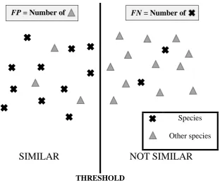
2.6 Fitness Evaluation

The fitness of the chromosome is evaluated using by means of false positive and false negative classification of species in the training set as shown in the Table 1.

Table 1- Matrix for false positive and false negative classification

Predicted

Positive Negative

Actual

Positive True Positive (TP)

False Negative (FN)

Total Number of Positive NP = TP + FN

Negative

False Positive (FP)

True Negative (TN)

Total Number of Negative NN = FP + TN

(34)

34

Species Other species

SIMILAR

NOT SIMILAR

[image:34.595.155.468.68.327.2]

THRESHOLD

Figure 9 – Determining false positive and false negative classification

The objective function of this problem is minimization of the probability of false positive (PFP) and

minimization of probability of false negative (PFN) which is shown below:

𝑃𝑃𝐹𝐹𝐹𝐹 =𝐹𝐹𝑃𝑃/𝑁𝑁𝑁𝑁, (11)

and

𝑃𝑃𝐹𝐹𝐹𝐹= 𝐹𝐹𝑁𝑁/𝑁𝑁𝑃𝑃 (12)

where FP is the number of false positives, FN is the number of false negatives, NP is the number of positive classifications and NN is the number of negative classifications. PFP and PFN are computed for

each gene since one gene represents the threshold value for a specific spectral similarity measures.

Since PFP and PFN for each gene, or threshold value, are statistically independent, the fitness function

per chromosome can be written as:

𝑃𝑃𝑡𝑡𝑐𝑐𝑡𝑡𝑡𝑡𝑖𝑖𝐹𝐹𝐹𝐹= ∑ 𝑃𝑃𝐹𝐹𝐹𝐹,𝑖𝑖 𝑘𝑘 𝑖𝑖=1

𝑘𝑘 (13)

𝑃𝑃𝑡𝑡𝑐𝑐𝑡𝑡𝑡𝑡𝑖𝑖𝐹𝐹𝐹𝐹=∑ 𝑃𝑃𝐹𝐹𝐹𝐹,𝑖𝑖 𝑘𝑘 𝑖𝑖=1

𝑘𝑘 (14)

(35)

35

where k is the number of genes, which is equal to five, i.e. the five different spectral similarity measures. Fitness value close to zero corresponds to the better optimization of the threshold.

2.7 Selection

The selection is the process to select which chromosomes are preserved for the next generation. The selection algorithm assigns two attributes to every chromosome 𝑖𝑖 in the population: nondomination rank (𝑖𝑖𝑟𝑟𝑡𝑡𝑛𝑛𝑘𝑘) and crowding distance (𝑖𝑖𝑑𝑑𝑖𝑖𝑑𝑑𝑡𝑡𝑡𝑡𝑛𝑛𝑐𝑐𝑑𝑑).

The chromosomes in the next generation are chosen based on the rank after the non-dominated sorting. If two or more chromosomes have the same rank, then the individual from less crowded neighbourhood is chosen as illustrated in Figure 10. Further explanation on the non-dominated sort is given in Section 2.7.1 and on crowding distance in Section 2.7.2.

Figure 10 – Selection in NSGA-II (Deb et al., 2002)

2.7.1 Non-dominated Sort

Once the fitness values assigned to the chromosomes, they are sorted based on the non-dominated rule. Chromosome A is said to dominate B if A’s fitness value of one objective is no worse than the B’s and at least one of A’s fitness value is better than the B (Seshadri, 2006) .The example is shown in Table 2.

Parents

Offspring

F1

F2

F3

Rejected

Non-dominated sorting Crowding distance sorting

(36)

[image:36.595.165.390.479.705.2]

36

Table 2 - Example of non-dominated sorting

Fitness value

Objective 1 Objective 2

Chromosome A 0.1 0.2

Chromosome B 0.1 0.4

In Table 2, it is shown that chromosome A and chromosome B have same fitness value for objective 1. However, for objective 2, chromosome A has lower fitness value than chromosome B. In this case, chromosome A dominates chromosome B.

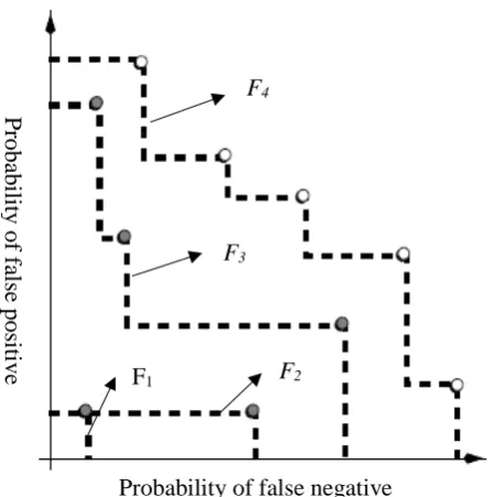
An illustration of the non-dominated sorting is shown in Figure 11 where F1, F2, F3, and F4 represent

fronts 1, 2, 3, and 4, respectively. The front means a set of solutions ranked by the closeness to the optimum solution. In this case, front 1 has the highest rank since it is the closest to the optimum solution which is the origin of the coordinate system. The optimum solution in this case refers to the minimization of false negative classification and minimization of false positive classification. The front 1 is also called the non-dominated front as other fronts are further from the optimum solution. The idea of non-dominated sorting emphasizes good attributes and ensure maintaining healthy chromosome.

Figure 11 – Illustration of Non dominated sorting (Zitzler, 1999) F4

F3

F2

F1

Probability of false negative

P

roba

b

ili

ty

of

f

al

se

pos

iti

(37)

37

2.7.2 Crowding Distance

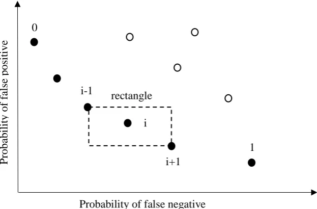
The purpose of crowding distance is to maintain the diversity of chromosomes in the population by selecting an individual from the less crowded neighbourhood. The level of crowding that surrounds a solution i is estimated by taking the average Euclidean distance between two solutions on either side of i on the same front. In Figure 12 the crowding distance of the i-th solution is the length of the longer

side of rectangle with the solution i-1 and i+1 defining its diagonal. Thus, greater crowding distance implies less crowded neighbourhood.

2.8 Crossover

1 0 1 1 0

0 1 1 0 1

Parent chromosomes

1 0 1 0 1

0 1 1 1 0

[image:37.595.145.457.266.471.2]

Child chromosomes

Figure 13 – Illustration of binary number crossover rectangle

0

1 i+1

i-1

i

P

roba

b

il

it

y

of

f

al

se

pos

it

ive

(38)

38

The genetic algorithm uses crossover and mutation to create children that are different from the parents. The crossover happens when two parents exchange their genetic parts to make two children as shown in Figure 13 for binary coded crossover. The main purpose of crossover is to increase the diversity of the population since the selection process as described in Section 2.7 reduces diversity. Another purpose is to preserve the mean of the population since the crossover is not dependent on fitness values.

In a binary coded GA chromosomes are fixed in length and the crossover operation is easier to implement and visualize. However, in this research, the chromosome is coded in real number and it is more challenging to define decision vector in real number to create new offspring. There are many variants of real-number-coded crossover operators, such as simulated binary crossover (SBX) introduced by Agrawal (1995), blend crossover (BLX-a) by Goldberg (1991), fuzzy recombination (FR) by Voigt et al. (1995), fuzzy connective based (FCB) by Herrera et al. (1997), unfair crossover by Nomura and Miyoshi (1996). In the study by Beyer and Deb (2000) shows that SBX, BLX, and FR crossover operators have similar performance and act as a mean-preserving operator, whereas, other crossover operators do not preserve the population mean. Therefore, the SBX is chosen in this research.

2.8.1 Simulated Binary Crossover

Unlike other real value crossover, SBX uses a probability distribution which is similar, in principle, to binary coded chromosome crossover. SBX is based on a single point crossover in binary coded GA. The binary coded crossover is given as:

𝑐𝑐1,𝑘𝑘 = 1₂�(1− 𝛽𝛽𝑘𝑘)𝑝𝑝1,𝑘𝑘+ (1 +𝛽𝛽𝑘𝑘)𝑝𝑝2,𝑘𝑘� (15)

𝑐𝑐2,𝑘𝑘= 1₂�(1− 𝛽𝛽𝑘𝑘)𝑝𝑝1,𝑘𝑘+ (1 +𝛽𝛽𝑘𝑘)𝑝𝑝2,𝑘𝑘� (16)

where 𝑐𝑐_𝑖𝑖_,_𝑘𝑘 is the 𝑖𝑖𝑡𝑡ℎ child with 𝑘𝑘𝑡𝑡ℎ component (k is gene element), 𝑝𝑝_𝑖𝑖_,_𝑘𝑘 is the selected parent chromosome and 𝛽𝛽_𝑘𝑘 is a random number with the density of:

(39)

39

𝑝𝑝(𝛽𝛽) = 1₂(𝜂𝜂𝑐𝑐+ 1)_𝛽𝛽𝜂𝜂𝑐𝑐+21 , if 𝛽𝛽> 1. (18)

This distribution, 𝛽𝛽, is obtained from uniformly sampled random number u between (0,1) and distribution index for crossover, 𝜂𝜂_𝑐𝑐, given as

𝛽𝛽(𝑢𝑢) = (2𝑢𝑢)(𝜂𝜂+11 ) , if u ≤ 0.5

(19) 𝛽𝛽(𝑢𝑢) = 1

[2(1−𝑢𝑢)](𝜂𝜂+11 ) , if u > 0.5

(20)

[image:39.595.164.418.347.578.2]

The distribution index, 𝜂𝜂_𝑐𝑐, is kept constant through the process. It determines how close the offspring is to the parents. Large 𝜂𝜂𝑐𝑐 means the offspring character is close to that of the parent and vice versa. This is illustrated in Figure 14.

Figure 14 - Probability of expanding and contracting depending on the value of ηc (Agrawal, 1995)

An illustration of the probability distribution of the offspring character resulting from SBX is given in Figure 15. It shows that the probability of obtaining a child whose character is closer to that of the parents is higher than the probability of obtaining a child whose character is completely different from that of the parents.

P

roba

b

il

it

y di

st

ri

b

ut

ion

ηc = 20

ηc = 2

ηc = 0

(40)

40

2.9 Mutation

Mutation alters one or more genetic values in the chromosome from its initial state. Similar to the crossover operators, the aim of mutation is to increase the diversity of the solutions. In the case of binary-coded GA, a mutation refers to randomly flipping the value of a gene, i.e. from 1 to 0 or vice versa, as shown in Figure 16.

1 0 1 0 1

Parent chromosome

1 0 0 0 1

Child chromosome

Figure 16- Illustration of binary number mutation

Mutation of binary-coded chromosomes can have a negative effect on finding an optimum solution as it may disrupt the optimization process (Deb, 2001). In the case of chromosomes being coded in real number Gaussian and polynomial mutation may be used to ensure higher probability of having offspring whose character is close to that of the parent. Deb and Deb (2014) found that there is no difference in the resulting probability distribution between Gaussian and polynomial mutation, and hence polynomial mutation is adopted in the current work.

P

ro

b

abi

li

ty

d

ens

it

y

of

t

he

of

fs

pr

in

g

𝑝𝑝1,𝑘𝑘 𝑝𝑝2,𝑘𝑘

(41)

41

Polynomial mutation was first introduced by Deb and Goyal (1996) and is based on the polynomial distribution:

𝑐𝑐𝑘𝑘= 𝑝𝑝𝑘𝑘+ (𝑝𝑝𝑘𝑘𝑈𝑈− 𝑝𝑝𝑘𝑘𝐿𝐿)𝛿𝛿𝑘𝑘 (21) where 𝑐𝑐_𝑘𝑘 is the offspring chromosome and 𝑝𝑝_𝑘𝑘 is the parent chromosome with 𝑝𝑝_𝑘𝑘𝑈𝑈 being upper bound, 𝑝𝑝𝑘𝑘𝐿𝐿 is the lower bound of the parent component and 𝛿𝛿𝑘𝑘 is deviation factor calculated from polynomial distribution as follows:

𝛿𝛿𝑘𝑘 = (2𝑟𝑟𝑘𝑘)

1

𝜂𝜂𝑚𝑚+1−1, if 𝑟𝑟_𝑘𝑘 < 0.5 (22)

𝛿𝛿𝑘𝑘 = 1−[2(1− 𝑟𝑟𝑘𝑘)]𝜂𝜂𝑚𝑚+11 _{, if}_𝑟𝑟_𝑘𝑘 _≥_0.5 (23)

where 𝑟𝑟_𝑘𝑘 is a randomly sampled number between 0 and 1 and 𝜂𝜂_𝑚𝑚 is mutation distribution index which is a user-defined parameter. This thesis uses 𝜂𝜂_𝑚𝑚 = 20 to maintain similar distribution spread of the offspring as crossover where 𝜂𝜂𝑚𝑚 = 20 is used. An example of the probability distribution of the offspring character that results from polynomial mutation is illustrated in Figure 16.

Figure 17 - The illustration of polynomial mutation

𝑝𝑝𝑘𝑘𝐿𝐿 𝑝𝑝𝑘𝑘 𝑝𝑝_𝑘𝑘𝑈𝑈

P

ro

b

abi

li

ty

d

ens

it

y

of

t

he

of

fs

pr

in

(42)

42

2.10 Output of Final Chromosome

(a) (b)

Figure 18 - The population in decision space (a) before NSGA-II, (b) after running 100th_generation

As shown in Figure 18 the population of the chromosomes or solutions converges to a single front in the decision space after many generations. The population is the pareto optimal line where some solutions favour false positive and some solutions favour false positive. The final chromosome, i.e. the solution that minimizes both probability of false negative and probability of false positive, is determined by finding the minimum misclassification rate as the Euclidean distance to the origin of the coordinate system of the decision space as shown in Figure 18.

𝑚𝑚𝑖𝑖𝑠𝑠𝑐𝑐𝑚𝑚𝑚𝑚𝑠𝑠𝑠𝑠𝑖𝑖𝑚𝑚𝑖𝑖𝑐𝑐𝑚𝑚𝑚𝑚𝑖𝑖𝑐𝑐𝑛𝑛𝑟𝑟𝑚𝑚𝑚𝑚𝑟𝑟= �𝑅𝑅𝐹𝐹𝐹𝐹2₊_{𝑅𝑅𝐹𝐹𝐹𝐹}2 ₍₂₄₎

0.1 0.2 0.3 0.4 0.5 0.6 0.7 0.8

0 0.1 0.2 0.3 0.4 0.5 0.6 0.7

Probability of false positive

0 0.05 0.1 0.15 0.2 0.25 0.3

Probability of false positive

RFP R_FN P roba b il it y of f al se pos it ive

(43)

43

2.11 Application to Evaluation Set and Parametric Studies

After the optimum parameters of the MOEA are identified using the training set, the parameters are then applied to the classification of species in the evaluation set.

In this thesis, different parameters were examined to compare the performance of unoptimized MOEA and that of optimized MOEA. The unoptimized MOEA is based on the default values described in Section 2.11.1, whereas, the optimized MOEA uses the best estimated values from a series of parametric study.

2.11.1 Unoptimized MOEA

[image:43.595.73.522.423.663.2]

The unoptimized MOEA uses the default values in NSGA-II as recommended in (Deb et al., 2000) Seshadri (2006) such as crossover rate of 0.9 and mutation rate of 0.1. The parameters for unoptimized MOEA are presented in Table 3 below.

Table 3 – Parameters for unoptimized MOEA

Variable representation Real number

Decision variable 5 (SAM, SCA, SID, SID-SAM, nSSM)

Population size 100 chromosomes

Number of generation 100 generations

Selection Non-dominated sorting and crowding distance Crossover operator Binary simulated crossover with rate of 0.9 Mutation operator Polynomial mutation with rate of 0.1

Performance measure The optimum of the final population i.e. the shortest distance to the origin (see Eq. (24))

2.11.2 Optimized MOEA

(44)

44

of MOEA when the parameters are varied and to find out which parameters significantly affect its performance. While there are many factors that may contribute to the performance of the MOEA, such as different type of crossover and mutation formulation, the following four parameters are considered to affect the performance of MOEA the most:

1. Number of generation;

2. Initialization of chromosomes; 3. Crossover rate; and

4. Mutation rate.

The first study covers the number of generation, which is considered one of significant factors affecting the performance of GA. If the number of generation is not sufficient, the search is terminated when optimum solution has not been reached. The study runs for 30 times on the training set which is chosen randomly from the spectral data and the result is taken as the average of the run. The optimum number is said to have reached convergence when there is 0.01% or less change in the solution. The study runs on initialization range of (𝑥𝑥̅ − 𝜎𝜎 to 𝑥𝑥̅+ 4𝜎𝜎), crossover rate of 0.9, and mutation rate of 0.1. Then, the optimum number of generation is then used for the next study.

In his thesis on statistical analysis of GA, Czarn (2008) argued that the initialization chromosome seeds can be a statistically significant factor in the MOEA result. Since initialization chromosome may interact with crossover and/or mutation rate, this parametric study uses 3-way ANOVA to test their significance. The study is performed with 4 different level initialization seeds, 4 different level of crossover rate, and 4 different level of mutation rate. So, in total, there are 43_{= 64 combinations. In}

(45)

45

power calculations were carried out using GPOWER (Erdfelder et al., 1996) assuming that the effect size is moderate yielded at least 7 runs per sample group.

(46)

46

Chapter 3 Results

“Life is short so it will be appreciated. We live to our fullest due to that”

Heiji Hattori

3.1 Result of Parametric Studies on MOEA Optimization

This section presents the results of the parametric studies described in Section 2.11 on optimization of MOEA, which focuses on four different parameters, i.e. number of generations (Section 3.1.1) , crossover rate, mutation rate, and initialization of chromosome (Section 3.1.2).

3.1.1 Number of Generations

As explained in Section 2.11.2, the number of generations is being investigated since MOEA requires sufficient generations to reach convergence before it is being terminated. The investigation results for determining the optimum number of generation are presented in Figure 20 for the six types of seagrass, and in Figure 21 for the four types of terrestrial plants.

(47)

47

(48)

48

Figure 21 - Effects of different number of generation to misclassification rate (terrestrial plants)

The result presented in Figure 21 shows that the terrestrial plants converge relatively faster than the seagrass species. The difference in the number of generations required for convergence might be attributed to the low variation in the terrestrial plant’s spectra reflectance. The eucalyptus converges after 190 generations, blackberry converges after 300 generations, lemon converges after 170 generations and cherry plum after 120 generations. These computed optimum numbers of generations are used in the subsequent study of finding optimum initialization of chromosome, crossover and mutation rate in Section 3.1.2.

3.1.2 Initialization of Chromosome, Crossover and Mutation Rate

(49)

49

3.1.2.1 Cymadocea serrulata

The result of 3-way ANOVA for Cymadocea serrulata is shown in Table 4. Table 4 – Result of 3-way ANOVA – Cymadocea serrulata

Source Sum Sq. d.f. Mean Sq. F Prob > F

Crossover 0.00087 3 0.00029 11.6 0

Mutation 0.00038 3 0.00013 4.99 0.007

Range 0.00044 3 0.00015 5.81 0.0034

Crossover * Mutation 0.00023 9 0.00003 1 0.461

Crossover* Range 0.0006 9 0.00007 2.65 0.0242

Mutation*Range 0.00031 9 0.00003 1.36 0.2559

Error 0.00068 27 0.00003

Total 0.00349 63

The result presented in Table 4 implies that the crossover rate, mutation rate, and initialization of chromosome are statistically significant. In addition, the ANOVA also finds that the interaction between crossover and range is significant. To ensure that this conclusion is correct, the study on normality of residuals and autocorrelation of residuals is presented in Figure 22.

(a) (b)

Figure 22 - (a) normal probability plot of residuals and (b) residuals versus fitted values – Cymadocea serrulata

(50)

50

(a) Contour plot with initialization range of 3 (b) Contour plot with mutation rate of 0.1

Figure 23 – Contour plot of misclassification rate – Cymadocea serrulata

The surface response contour plot in Figure 23(a) and (b) suggests that low misclassification rate favours high crossover rate, high mutation rate, and low initialization range for initial chromosome.

3.1.2.2 Halodue univervis

The result of three-way ANOVA for Halodue univervis is presented below in Table 5. Table 5 – Result of 3-way ANOVA – Halodue univervis

Crossover 0.00061 3 0.0002 40.12 0

Mutation 0.00005 3 0.00002 3.45 0.0304

Range 0.00005 3 0.00002 3.17 0.0402

Crossover * Mutation 0.0001 9 0.00001 2.09 0.067

Crossover* Range 0.00003 9 0.00001 0.62 0.7726

Mutation*Range 0.0008 9 0.00001 1.74 0.1291

Error 0.00014 27 0.00001

Total 0.00105 63

(51)

51

(a) (b)

Figure 24 – (a) normal probability plot of residuals and (b) residuals versus fitted values – Halodue univervis

The normal probability plot of residuals in Figure 24(a) and plot of residuals versus fitted values appear to be satisfactory. Hence, there can be ascertained that the conclusion of ANOVA is valid. Then, the response surface contour plots (Figure 25) are generated using regression model to analyse the parameters.

Figure 25 - Contour plot of misclassification rate – Halodue univervis

(52)

52

3.1.2.3 Halophia ovalis

The outcome of three-way ANOVA test for Halophia ovalis is presented in Table 6. Table 6 - Result of 3-way ANOVA – Halophia ovalis

Crossover 0.00276 3 0.00092 92.87 0

Mutation 0.00012 3 0.00004 4.08 0.0164

Range 0.00073 3 0.00024 24.65 0

Crossover* Range 0.00061 9 0.00007 6.83 0

Mutation*Range 0.00014 9 0.00002 1.53 0.1879

Error 0.00027 27 0.00001

Total 0.00473 63

The result of ANOVA indicates that the crossover rate, mutation rate, and initialization range are statistically significant to the misclassification rate. There is also significant interaction between the crossover rate and initialization range. To confirm if the ANOVA is valid, the normality analysis on the residuals and the non-correlation among the variables on the residuals are presented below in Figure 26.

(a) (b)

Figure 26 – (a) normal probability plot of residuals and (b) residuals versus fitted values – Halophia ovalis

(53)

53

Figure 27 - Contour plot of misclassification rate – Halophia ovalis

The response surface contour plot shown in Figure 27 displays that low misclassification favours high crossover rate, low mutation rate, and low initialization range.

3.1.2.4 Halophia spinulosa

The 3-way ANOVA test for Halophia spinulosa is shown in Table 7. Table 7- Result of 3-way ANOVA – Halophia spinulosa

Crossover 0.00023 3 7.67E-5 22.4 0

Mutation 0.00005 3 1.58E-5 4.61 0.0099

Range 0.00005 3 1.69E-5 4.94 0.0073

Crossover * Mutation 0.00006 9 6.66E-6 1.95 0.0873

Crossover* Range 0.00004 9 4.68E-6 1.37 0.2506

Mutation*Range 0.00002 9 2.40E-6 0.7 0.7015

Error 0.00009 27 3.42E-6

Total 0.00054 63

(54)

54

(a) (b)

Figure 28 – (a) Normal probability plot for residuals and (b) residuals versus fitted value – Halophia spinulosa

Both normal probability plot of residuals and plot of residuals versus fitted values in Figure 28. These plots appear to be satisfactory, so there can be ascertained that the conclusion of ANOVA is valid. The response surface that explains the relation of the parameters to the misclassification rate is shown in Figure 29.

Figure 29 - Contour plot of misclassification rate – Halophia spinulosa

(55)

55

3.1.2.5 Syringodium isoetofolium

The result of 3-way ANOVA for Syringodium isoetofolium is presented in Table 8 below. Table 8 - Result of 3-way ANOVA – Syringodium isoetofolium

Crossover 0.00072 3 0.00024 18.7 0

Mutation 0.00015 3 0.00005 3.89 0.0196

Range 0.00182 3 0.00061 47.36 0

Crossover* Range 0.0001 9 0.00001 0.84 0.5883

Mutation*Range 0.00017 9 0.00002 1.49 0.2028

Error 0.00035 27 0.00001

Total 0.00338 63

The ANOVA result shows that all three measured parameters i.e. crossover rate, mutation rate and range are statistically significant. However, there are no significant interaction among the parameters. The investigation on the assumptions of ANOVA is shown in Figure 30.

(a) (b)

Figure 30- (a) normal probability plot of residuals and (b) residuals versus fitted values – Syringodium isoetofolium

(56)

56

Figure 31 – Contour plot of misclassification rate – Syringodium isoetofolium

Figure 31a shows the response surface contour plot when the initial chromosomes starts with range (𝑥𝑥̅ − 𝜎𝜎 to 𝑥𝑥̅+𝑚𝑚𝜎𝜎) where m is 3. Figure 31 is the response surface contour plot when the mutation rate is 0.1. Both contour indicate that minimization of misclassification rate requires crossover rate and mutation rate to be high and initialization range to be low.

3.1.2.6 Zostera muelleri

The result of three-way ANOVA is shown below in Table 9.

Table 9 - Result of 3-way ANOVA – Zostera muelleri

Crossover 0.00025 3 8.48E-5 13.15 0

Mutation 0.00001 3 3.21E-6 0.5 0.686

Range 0.00016 3 5.32E-5 8.26 0.0005

Crossover * Mutation 0.00008 9 8.69E-6 1.35 0.2598

Crossover* Range 0.00002 9 2.52E-6 0.39 0.9283

Mutation*Range 0.00007 9 7.57E-6 1.17 0.3495

Error 0.00017 27 6.44E-6

Total 0.00077 63

(57)

57

(a) (b)

Figure 32- (a) normal probability plot of residuals and (b) residuals versus fitted values – Zostera muelleri

The normal probability of residuals and residuals versus fitted values plots in Figure 32 confirm the valid conclusion of ANOVA. To analyse the relation of the significant parameters, the response surface and contour plot are generated by regression model which are shown in Figure 33. Since the mutation rate is found to be non-significant, therefore the response surface can be plotted with crossover rate and initialization range variables in Figure 33(a).

(a) Response surface (b) Contour plot

Figure 33 – (a) Response surface and (b) contour plot of misclassification rate – Zostera muelleri

Figure 33 indicates that the low misclassification rate favours high crossover rate and high initialization range.

3.1.2.7 Eucalyptus

(58)

[image:58.595.72.525.315.507.2]

58

Table 10 - Result of 3-way ANOVA – Eucalyptus

Crossover 0.00233 3 0.00078 64.15 0

Mutation 0.00059 3 0.0002 16.21 0

Range 0.00016 3 0.00005 4.37 0.0124

Crossover* Range 0.00013 9 0.00001 1.21 0.3275

Mutation*Range 0.00016 9 0.00002 1.49 0.2018

Error 0.00033 27 0.00001

Total 0.00382 63

The ANOVA result indicates that the statistical significant correlation of crossover rate, mutation rate, and initialization range towards misclassification rate. However, there is no statistical significance between the parameters. The examination of ANOVA’s validity is presented in Figure 34.

(a) (b)

Figure 34- (a) normal probability plot of residuals and (b) residuals versus fitted values – Eucalyptus

(59)

59

[image:59.595.76.525.71.266.2]

Figure 35 – Contour plot of misclassification rate - Eucalyptus

The surface response contour plots in Figure 35(a) and (b) imply that the minimization of misclassification rate requires high crossover rate, high mutation rate, and low initialization range (m = 3).

3.1.2.8 Blackberry

The result of three-way ANOVA for blackberry is shown below in Table 11. Table 11- Result of 3-way ANOVA – Blackberry

Crossover 0.00726 3 0.00242 44.95 0

Mutation 0.00076 3 0.00025 4.69 0.0092

Range 0.00135 3 0.00045 8.33 0.0004

Crossover* Range 0.00034 9 0.00004 0.71 0.6969

Mutation*Range 0.00079 9 0.00009 1.62 0.1596

Error 0.00145 27 0.00005

Total 0.01234 63

[image:59.595.74.523.445.565.2]

(60)

60

[image:60.595.75.525.71.264.2]

(a) (b)

Figure 36 - (a) normal probability plot of residuals and (b) residuals versus fitted values – Blackberry

Figure 36(a) shows slight skew on the normal probability plot of residuals. A further investigation using Jarque-Bera test shows that the normality distribution is not violated. The residuals versus fitted plot in Figure 36(b) appears to be satisfactory. Therefore, there is no doubt about the validity of ANOVA. The response surface contour plots as displayed in Figure 37 show the relations of the parameters to the misclassification rate.

Figure 37 - Contour plot of misclassification rate – Blackberry

[image:60.595.75.524.418.602.2]

(61)

61

3.1.2.9 Lemon (Citrus limon)

[image:61.595.73.525.146.268.2]

The result for three-way ANOVA for lemon is presented below in Table 12. Table 12- Result of 3-way ANOVA – Lemon

Crossover 5.39E-5 3 1.79E-5 89.27 0

Mutation 1.79E-6 3 5.98E-7 2.97 0.0496

Range 1.02E-6 3 3.41E-7 1.69 0.1917

Crossover * Mutation 3.90E-6 9 4.33E-7 2.15 0.0601

Crossover* Range 1.46E-6 9 1.63E-7 0.81 0.6115

Mutation*Range 1.80E-6 9 2.01E-7 1.01 0.4654

Error 5.44E-6 27 2.01E-7

Total 6.94E-5 63

The ANOVA result shows that only crossover and mutation rate are significant to the misclassification rate. In order to ascertain the assumptions of ANOVA are valid, the normal probability plot of residuals and residuals versus fitted values plot are displayed in Figure 38.

[image:61.595.75.526.371.564.2]

(a) (b)

Figure 38 - (a) normal probability plot of residuals and (b) residuals versus fitted values – Lemon

(62)

62

[image:62.595.72.523.73.266.2]

(a) Response surface (b) Contour plot

Figure 39 – (a) Response surface and (b) contour plot of misclassification rate – Lemon

The surface response and contour plot in Figure 39 suggest that the minimization of misclassification rate favours the high crossover rate and low mutation rate. In this case, the crossover rate is to be 1, and mutation rate to be 0.1.

3.1.2.10 Cherry Plum

The result for a three-way ANOVA test on Cherry plum is shown below in Table 13. Table 13 - Result of 3-way ANOVA – Cherry plum

Crossover 1.40E-5 3 4.69E-6 36.32 0

Mutation 2.76E-6 3 9.20E-7 7.1 0.0011

Range 1.21E-6 3 4.03E-7 3.12 0.0426

Crossover * Mutation 3.13E-6 9 3.48E-7 2.69 0.0224

Crossover* Range 2.43E-6 9 2.70E-7 2.09 0.0678

Mutation*Range 1.86E-6 9 2.07E-7 1.6 0.165

Error 3.49E-6 27 1.29E-7

Total 2.90E-5 63

[image:62.595.73.522.441.563.2]

Hyperspectral classification optimization using multiobjective evolutionary algorithm