Strongly overdamped dissipative particle dynamics for fluid-solid systems

Strongly Overdamped Dissipative Particle Dynamics for

Fluid-Solid Systems

N. Phan-Thien

, N. Mai-Duy

, B.C. Khoo

, and D. Duong-Hong

1

_{Department of Mechanical Engineering, Faculty of Engineering,}

National University of Singapore, Singapore.

2

_{Computational Engineering and Science Research Centre,}

School of Mechanical and Electrical Engineering,

University of Southern Queensland, Toowoomba, QLD 4350, Australia.

3

_{Welch Allyn Singapore Pte. Ltd.,}

438B Alexandra Road, #01-03 Alexandra Technopark, Singapore 119968

Submitted to

Applied Mathematical Modelling

, 5/Feb/2015; revised,

8/Nov/2015;

revised (2), 4/Dec/2015

Abstract In this paper, a numerical scheme is used to study strongly-overdamped

Dissi-pative Particles Dynamics (DPD) systems for the modelling of fluid-solid systems. In the

scheme, the resultant set of algebraic equations for the velocities are directly solved in an

iterative manner. Different test problems, e.g., viscometric flows, particulate suspensions

and flows past a periodic square array of cylinders, are used to verify the proposed method.

In the simulation of particulate suspensions, a new simple model for massless suspended

particles is presented. A DPD fluid in the overdamped limit is shown to possess several

attractive properties including much faster dynamic response and near-incompressibility.

Keywords: Dissipative Particles Dynamics, strongly overdamped systems, compressibility,

dynamic response, particulate suspension

1

Introduction

Dissipative Particles Dynamics (DPD) is a particle-based method originally designed for the

simulation of complex fluids on mesoscopic length scale [1-5]. In DPD, a fluid is modelled by

a system of particles interacting with each others through pairwise forces. These particles are

supposed to model the fluid behaviour (viscous, or otherwise dictated by the specification of

the microstructure connectivity) when seen in a representative volume. Objects suspended

in the fluid, e.g., rigid particles and droplets, can also be represented by DPD particles with

appropriate forms of interactions. These features make the DPD method (and its variants)

very attractive in the modelling of complex fluid systems. DPD has been used with varying

degrees of success to simulate various problems: particulate suspensions, emulsions, polymer

solutions, polymer melts, red blood cell modelling, etc.

In [6], the equivalent Poisson ratio of a DPD fluid (a measure of compressibility) in the

absence of conservative forces was estimated as 0.24, and measured in a simulated four-rolled

mill at a value of 0.48 (at best), less than the incompressible limit of 0.5. This compressibility

nature of a DPD fluid implies that unwanted effects due to compressibility of a DPD flow

will occur, and special care is needed in interpretation of the flow results, especially at

high Re number. The Mach number, which is the ratio of a characteristic velocity of the

fluid to its sonic velocity, can also be used to estimate the effects of compressibility. The

fluid flow may be considered weakly compressible (or nearly incompressible) when the flow

Mach number is less than 0.3. Another past issue is the Schmidt number, the ratio of the

diffusion of momentum to the diffusion of mass in a fluid, governing the dynamic response

of a fluid. For a standard-parameter DPD fluid, the Schmidt number is of the order unity.

For a real water-like fluid, the Schmidt number is O(103_{), and there is the need to improve}

on the dynamic behaviour of the DPD system. By some slight modifications to its standard

parameters, a DPD fluid could be designed to have a Schmidt number of O(103_{) [7].}

The Reynolds (Re), Mach (M) and Schmidt (Sc) numbers are defined as [5]

Re= mnUL

η ; M =

U cs

, c2s =

kBT

m +

π 15

anr4

c

m ; Sc=

η

where U is a flow characteristic velocity, L a flow characteristic length, m the mass of the

particle, n the number density, η the dynamic viscosity, cs the speed of sound, kBT the

Boltzmann temperature (mean kinetic energy of the particles), a the repulsion coefficient,

rc the cut-off radius for the particles interactions, and D the fluid diffusion coefficient. It

is therefore possible to control the three quantities Re, M and Sc collectively by means of

m. A strongly overdamped system results with the limit of m → 0; the limit corresponds

to Re → 0, M → 0 and Sc → ∞. This limit also corresponds to the inertial time scale

mγ−1 _{→0 (γ the coefficient characterising the strength of the dissipative force, refer to (3)}

below). It is noted that highly overdamped Brownian dynamics systems and their behaviour

have been extensively studied and well established, but no such studies exist for overdamped

DPD systems. In [8,9], the use of low mass was proposed in the DPD modelling of slow

(creeping) flow in which high sonic speed, low Reynolds and high Schmidt numbers are

achieved altogether. This comes at the expense of solving stiff stochastic differential

equa-tions for which exponential time differencing (ETD) schemes may be more efficient than

standard solvers. In [10], the overdamped limit for a simple DPD system was investigated,

where DPD particles are of the same type and the imposed boundary conditions are all

periodic. The resultant system matrix has zero row and zero column sums, corresponding to

a loss of second-order time derivatives, and a multiplicity of solutions (each solution differs

from the other by a rigid-body motion). It was shown that a possible and practical

itera-tive solution scheme is to add to the original system the eigenvectors weighted by the inner

product formed from the eigenvectors and the solution vector (which is in fact the constraint

of zero center of mass velocity) - this later step was recognised as a Wielandt’s deflation

technique.

The present work is an extension of our previous study of strongly-overdamped DPD, with

included movable and stationary solid bodies, also modelled using a subset of DPD particles.

It will be shown that the velocity constraints on stationary particles render a unique solution

to the system without the need for Wielandt’s deflation. Emphasis will be placed on: (i) the

effects of using frozen particles on the flow; (ii) the effects of including physical constraint of

constant velocity of the mass centre in the DPD system; and (iii) the modelling of massless

suspended particles. Basic DPD equations in the overdamped limit are given in Section 2.

in Section 4. Section 5 gives some concluding remarks.

2

DPD equations for strongly overdamped systems

The DPD equations can be written as

dr_i

dt =vi, (2)

mi

dvi

dt =

N

X

j=1,j6=i

aijwCeij − N

X

j=1,j6=i

γwD(eij ·vij)eij + N

X

j=1,j6=i

σwRθijeij, (3)

where i= (1,2,· · · , N), N is the number of particles, mi, ri and vi the mass, position and

velocity vector of the ith particle, t the time, vij = vi −vj, eij = rij/rij (rij = ri −rj,

rij =|rij|), aij, γ and σ are constant parameters, wC, wD and wR are the weight functions

that vanish ifrij ≥rc, and θij a Gaussian white noise (θij =θji) with stochastic properties

hθiji= 0, (4)

hθij(t)θkl(t′)i= (δikδjl+δilδjk)δ(t−t′),withi6=k and j 6=l. (5)

The first term on the right side of (3) is the conservative force (Fij,C), the second the

dissipative force (Fij,D) and the last the random force (Fij,R). The equilibrium and detailed

balance (Fluctuation-Dissipation theorem, [2]) of the system requires

wD(rij) = (wR(rij))2, (6)

kBT =

σ2

2γ, (7)

where kBT is the Boltzmann temperature (mean kinetic energy of the particles). In this

study, we take the weighting functions in the form wC(rij) = 1 − rij/rc and wD(rij) =

(1−rij/rc)1/2. It is noted that the exponent in the expression for wD is taken to be 1/2

instead of 2 to increase theSc number by a factor of 10 and thereby improve on the dynamic

response of the DPD fluid [7]. The DPD forces are centre-to-centre and thus both linear

that DPD particles interact through a soft potential, the simulation can be carried out on

length and time scales far beyond those associated with molecular dynamics (MD). Viscous

interactions are accounted for by dissipative forces depending on the relative velocity of the

particle.

Calculation of mean quantities

The flow domain is divided into bins which are used to collect local data. The

assuming-ergodic flow properties are calculated by time averaging over all sampled data in each bin.

The fluid density and linear momentum are, respectively, defined as

ρ(r, t) = *

X

i

mδ(r−ri)

+

, (8)

ρ(r, t)u= *

X

j

mvjδ(r−rj)

+

. (9)

The stress tensor is found for a microscopic system of particles by the Irving-Kirkwood

method

T=−n *

X

i

mV_iV_i+1 2

X

i

X

j6=i

r_ij(F_ij,C +F_ij,D) +

, (10)

where Vi = vi −u is the peculiar velocity of particle i with respect to the mean field

velocity u and h.i denotes the ensemble average. The sums on the right side of (10) denote

the contributions to the stress from the momentum transfer of DPD particles and from the

interaction forces, respectively. The pressure can be defined as the trace of the stress tensor

p=−1

3trT. (11)

It is noted that these mean quantities satisfy conservation laws:

∂

∂tρ(r, t) +∇ ·(ρ(r, t)u(r, t)) = 0, ∇=∂/∂r, (12)

and

∂

∂t (ρu) +∇ ·(ρuu) = ∇ ·T. (13)

(12)-(13). Adopting this particle-based point of view, DPD particles may be thought of as a

model of a behaviour (e.g., viscous compressible fluid), not merely particles of some exclusion

sizes. More details can be found in [5,11], for instance.

Strongly overdamped DPD systems: In the overdamped limit (m/γ2 _{→ 0), equation}

(3) reduces to a balance of forces

N

X

j=1,j6=i

γwDeijeij ·(vi−vj) = N

X

j=1,j6=i

aijwCeij + N

X

j=1,j6=i

σwRθijeij. (14)

3

Proposed numerical procedure

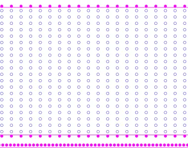
Consider a DPD system as shown in Figure 1. In the wall regions, as represented by two

boxes, top and bottom, the wall particles, numbered Nw, are frozen. We can arbitrarily

number the DPD particles consecutively as i = 1, . . . , Ns, Ns + 1, . . . , N, where Ns is the

number of DPD particles representing the fluid (the solvent), and N = Ns+Nw the total

number of DPD particles. Initially, the fluid particles are distributed uniformly, and their

velocities are generated randomly with a zero sum in all directions.

We construct the DPD system by lettingi taking values from 1 to Ns in (14)

Av=f, (15)

where A is the system matrix, v the column vector of unknown velocity vectors and f the

column vector of right hand force vectors and part of the original left hand matrix multiplied

by known velocity vectors:

A=          PN

j=2γwDe1je1j −γwDe12e12 · · · −γwDe1Nse1Ns −γwDe21e21 PN_j=1,j6=2γwDe2je2j · · · −γwDe2Nse2Ns

... ... . .. ...

−γwDeNs1eNs1 −γwDeNs2eNs2 · · ·

PN−1

j=1 γwDeNsjeNsj          , (16)

v= (v1,v2,· · · ,vNs)

T

f =          PN

j=2a1jwCe1j +

PN

j=2σwRθ1je1j

PN

j=1,j6=2a2jwCe2j +PNj=1,j6=2σwRθ2je2j

... PN−1

j=1 aNsjwCeNsj + PN−1

j=1 σwRθNsjeNsj          +          PN

j=Ns+1γwDe1je1jvj PN

j=Ns+1γwDe2je2jvj ...

PN

j=Ns+1γwDeNsjeNsjvj          . (18)

Since the known velocity vectors, corresponding to the wall particles, on the left side of (14)

are moved to the right side (the last term in (18)), the row and column sums of the system

matrix A are no longer zero and consequently, the problem of multiple solutions due to a

rigid-body motion is no longer a concern. It can be seen that A is a sparse matrix because

the construction of rows of this matrix involves only particles within the interaction zone.

Below are two iterative schemes for solving the system Av = f. They are applicable for

2D and 3D space. In Scheme 2, the Wielandt’s deflation method is utilised to reduce the

spectral radius (faster convergence). In this regard, Scheme 2 is expected to be more efficient

than Scheme 1.

3.1

Scheme 1

We decompose the system (15) into

Iv+Kv=f, (19)

where I =          PN

j=2γwDe1je1j 0 · · · 0

0 PN_j=1,j6=2γwDe2je2j · · · 0

..

. ... . .. ...

0 0 · · · PN_j=1−1γwDeNsjeNsj          , (20) and K=         

0 −γwDe12e12 · · · −γwDe1Nse1Ns

−γwDe21e21 0 · · · −γwDe2Nse2Ns

... ... . .. ...

−γwDeNs1eNs1 −γwDeNs2eNs2 · · · 0

The inverse ofI can be computed in the following form

I−1 =          PN

j=2γwDe1je1j

−1

0 · · · 0

0 PN_j=1,j6=2γwDe2je2j

−1

· · · 0

... ... . .. ...

0 0 · · · PN_j=1−1γwDeNsjeNsj

−1          . (22)

Multiplying both sides of (19) byI−1 _{results in}

v+Hv=b, (23)

where H = I−1_{K and b = I}−1_{f. To solve (23), a simple Picard’s iteration scheme can be}

used

vl_i =−Hivl−1+bi, (24)

wherei= (1,2,· · · , Ns),

Hi = N

X

j=1,j6=i

γwDeijeij

!−1

−γwDei1ei1,· · · ,−γwDei(i−1)ei(i−1),0,−γwDei(i+1)ei(i+1),· · · ,−γwDeiNseiNs

, (25)

and

b_i =

N

X

j=1,j6=i

γwDeijeij

!−1 _N

X

j=1,j6=i

aijwCeij + N

X

j=1,j6=i

σwRθijeij + N

X

j=Ns+1

γwDeijeijvj

! .

(26)

The iterative process stops when the following convergence measure is satisfied

norm(vl−vl−1)<10−7norm(vl), (27)

where the notation norm is used to denote the Euclidean distance.

A first-order Euler algorithm is employed here

rk_i+1 =rk_i +vk_i∆t, (28)

where ∆t=tk+1_−tk_.

Now we investigate the effects of frozen particles in the wall regions on the flow. Consider

the ith wall particle (i= (Ns+ 1,· · · , N)). Its motion is governed by

mdvi dt =

N

X

j=1

(Fij,C +Fij,D+Fij,R) +Fi,W, (29)

where Fi,W is the constraint (reaction) force from the ground/base. Since the particle i is

frozen (v_i =0), the constraint force on it is computed as

F_i,W =−

N

X

j=1

(F_ij,C +F_ij,D+F_ij,R). (30)

The total force exerted on the DPD system from the base is thus given by

e

F=

N

X

i=Ns+1

Fi,W =− N

X

i=Ns+1

N

X

j=1

(Fij,C+Fij,D+Fij,R) = Ns X i=1 N X j=1

(Fij,C+Fij,D+Fij,R).

(31)

It can be seen that the total force exerted on the fluid region from the walls is also Fe.

The centres of mass of the fluid interior and the wall particles are given by

mNsRsc = Ns X

i=1

mr_i, mNwRwc = N

X

i=Ns+1

mr_i. (32)

Note that (i) the centre of mass of the whole DPD system is

NRc =NsRcs+NwRwc; (33)

and (ii) the three centres are initially located at the origin with zero velocities.

In the present system, there are two types of forces, the DPD and reaction forces. The

which are forces exerted on the frozen forces from the ground/base, do not cancel out. As a

result, the mass centre of the system/fluid region will not move at constant (zero) velocity

any longer. Consider a domain of 10×10 in reduced units (10×12 if the two wall regions

are included) as shown in Figure 1. We employ the standard DPD parameters: aij = 18.5,

n = 4, σ = 3, rc = 1 and kBT = 1, and take ∆t = 0.005. The number of particles in the

fluid region are 400. In each wall region, there are two boundary layers on which 20 and

50 uniformly-distributed fixed particles are employed. The total number of particles used

are thus 540. It is observed that (i) velocity components of the mass centre are oscillatory

with zero mean and magnitude in the range of -15 to 15 for the x component and of -8 to

8 for the y component; (ii) the location of the mass centre moves far away from its original

position and displacements in the x direction are much larger than in the y direction (for

2500 time steps, −0.6< xcm <1.2 and −0.1 < ycm <0.1); and the total of reaction forces

also fluctuates with zero mean. It appears that the reaction forces are transmitted into the

fluid region, just like “external forces”, producing some fluid motion, which is a consequential

artefact of the wall constraints.

3.2

Scheme 2

In this scheme, the DPD system incorporates the physical constraint of constant velocity of

the centre of mass in order to enhance the efficiency of the iterative solving process as well

as to offset against the fluid motion induced by constraint forces.

We now introduce the relative motion of the particles

xi =ri−Rcs, i= (1,· · · , Ns). (34)

Differentiating equation (34) with respect to time twice and making use of (3), (32), (30)

and (31) yield

mx¨i = N

X

j=1,j6=i

(Fij,C +Fij,D+Fij,R)−

1 Ns

e

F. (35)

This relative motion of fluid DPD particles (equivalent to describing the motion in a frame

is now guaranteed to have their centre of mass in this moving frame stationary. It should

be emphasised that the new force term in (35) is only present with wall particles, when a

transmission of forces from the wall to the fluid region occurs. If there are no wall particles,

these reaction forces are zero, and this mentioned force field vanishes. The sum of all forces

exerted on the DPD system completely vanishes.

Let the fluid density and linear momentum in the moving frame, respectively, be defined as

ρ(x, t) = *

X

i

mδ(x−xi)

+

, (36)

ρ(x, t)u= *

X

j

mx˙jδ(x−xj)

+

. (37)

Note thatr=x+Rs_c and r_i =x_i+Rs_c, and thus r−r_i =x−x_i. Equation (8) becomes

ρ(r, t) = *

X

i

mδ(r−ri)

+ =

* X

i

mδ(x−xi)

+

=ρ(x, t). (38)

Note thatr =x+Rs_c andrj =xj+Rsc, and thusvj =x˙j+R˙sc andr−rj =x−xj. Equation

(9) becomes

ρ(r, t)u= *

X

j

mvjδ(r−rj)

+

= *

X

j

mx˙jδ(x−xj)

+ +

* X

j

mR˙s_cδ(r−rj)

+

=ρ(x, t)u+ *

X

j

mR˙s_cδ(r−r_j) +

, (39)

where the second term on the right side of (39) can be regarded as the side effect of freezing

the wall particles. One expects this term to approach zero as the number of time steps used

for the time averaging process increases (in the case when periodic boundary conditions are

applied, this can be demonstrated to be zero). The velocityuto be determined is the wanted

part of the velocity u.

Note that ri = xi +Rsc, rj = xj +Rsc, vi =x˙i+R˙sc and u =u+hR˙sci, and thus rij = xij

andVi =vi−u=Vi+

˙

i in the relative motion. Equation (10) can be rewritten as

T=−n *

X

i

mViVi+

1 2

X

i

X

j6=i

rij(Fij,C +Fij,D)

+ ,

=−n *

X

i

mViVi+

X

i

mR˙s_c − hR˙s_ci R˙s_c− hR˙s_ci+ 1 2

X

i

X

j6=i

xij(Fij,C +Fij,D)

+ .

(40)

Owing to the facts that (i) R˙s_c − hR˙s_ci is not spatial dependent and (ii) only the pressure

gradient (not the pressure itself) matters in the momentum balance equation, the stress

tensor computed in the moving frame is in fact the stress tensor (10) modulo an un-important

isotropic pressure term. Expressions (38), (39) and (40) are valid for any value ofm.

With the presence of frozen wall particles, the motion of DPD particles in reference to

the centre of mass is a better means of representation of the flow as the artefacts of the

wall constraints are absent. The centre of mass of the present system has constant (zero)

velocities. Hereafter, for the sake of simplicity, notations for the position, velocity, etc., in

the moving frame are taken to be the same as those in the fixed frame. Furthermore, the

DPD formulation can now be reformulated with the help of Wielandt’s deflation method

[12,13] to deflate the largest value of the eigenvalues of the matrixH and thus to reduce the

spectral radius (faster convergence)

v+Hv+ǫ_x[v,ǫ_x] +ǫ_y[v,ǫ_y] +ǫ_z[v,ǫ_z] =be, (41)

where [·,·] denotes the natural inner product of two vector elements in the underlying space,

ǫ_x = U_x,U_x, ...,U_x)T pN_sU_x, U_x = (1,0,0)T, U2

x =Ux·Ux, (42)

ǫ_y = (U_y,U_y, ...,U_y)T pN_sU_y, U_y = (0,1,0)T, U2

y =Uy ·Uy, (43)

ǫ_z = (U_z,U_z, ...,U_z)T pN_sU_z, U_z = (0,0,1)T, U2

z =Uz·Uz, (44)

and

e

b=b+I−1(− 1

Ns

e

F,· · ·,− 1

Ns

e

F

| {z }

Ns

The last three terms on the left of (41) represent the constraint of zero velocity of the centre

of mass [10] and therefore they do not contribute to the governing equation.

To solve (41), a simple Picards iteration scheme can be used

v_il=−Hivl−1−ǫ_xhvl−1,ǫ_xi −ǫ_yhvl−1,ǫ_yi −ǫ_zhvl−1,ǫ_zi+be_i, (46)

wherei= (1,2,· · · , Ns). Note that equation (23) of Scheme 1 and equation (46) of Scheme

2 can be constructed and solved in parallel to enhance the computational efficiency.

Numerical results obtained show that the velocity field has a zero sum (i.e.,<10−8_{) in each}

direction as the scheme is designed to do so. Also, as expected, the centre of mass is observed

to be stationary (i.e. |xc|,|yc|<10−10).

4

Numerical examples

The proposed two schemes are verified in 2D flows: Couette flows, flows past a periodic square

array of cylinders and particulate suspensions. The flows are modelled using a DPD system

in two dimensions with the following standard parameters: aij = 18.5, n= 4, σ = 3,rc = 1

andkBT = 1. Cutoff radius and Boltzmann temperature are commonly normalized to unity.

Repulsion parameter aij is chosen from the requirement that the DPD fluid is supposed to

have the same isothermal compressibility to that of water. For the modelling of single phase

systems, DPD is known to possess a scale-free property over the whole mesoscopic range.

The larger the number of fluid molecules packed into a DPD particle (larger DPD particle),

the higher the coarse graining level will be. With an appropriate scaling scheme, numerical

results from solving the DPD equations of motion can be independent to the number density

chosen. The noise level σ = 3 is recommended as its larger values may render the system

unstable. Under these values, fast simulations (∆t = O(10−3_)−O(10−2_{)) can be achieved}

[4]. In the present work, we employ a time step in the range of 0.005 to 0.01 and observe that

the temperature is maintained constant. In solving the velocity DPD equation, the Picards

4.1

Couette flow

This example is chosen to study the performance of Scheme 1 and Scheme 2. Consider a flow

in the space between two horizontal parallel plates, Lx×Ly = 10×10. The two plates are

sliding in opposite directions of a speed U = 10. We impose periodic boundary conditions

on the left and right boundaries of the flow domain and the velocity U = (±U,0)T _{on the}

wall frozen particles. Before the simulation is started, the DPD particles are allowed to

equilibrate from a uniform configuration and initial velocities are chosen in such a way that

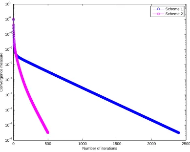
their sums in all directions are zero. Both Scheme 1 and Scheme 2 are employed. Figure 2

shows Scheme 2 converges much faster than Scheme 1 for a given time step. With a given

tolerance of 10−7_{, the Picard algorithm typically requires about 2100 iterations for Scheme}

1 and about 450 iterations for Scheme 2. The ratio of the CPU time required for Scheme 1

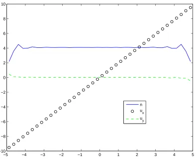
to that of Scheme 2 is about 3.65. Figure 3 displays the distribution of number density and

velocities on the flow cross section by Scheme 2. It can be seen that an approximately linear

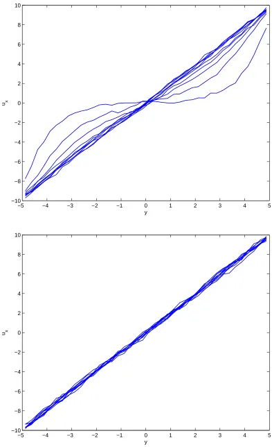
velocity profile is obtained. In Figure 4, we compare the development of the x−component

velocity profile between two cases: m = 0 (overdamped) and m = 1 (standard), revealing

that the DPD fluid in the overdamped limit has a much faster dynamic response.

4.2

Flow past a periodic square array of fixed cylinders

This example is chosen to investigate compressibility of the overdamped DPD system.

Be-cause of periodicity, one can replace the infinite domain with a finite one containing only

one cylinder to analyse the flow (Figure 5). Assume that the motion of a fluid is driven by

a pressure drop in the x direction. Using Fourier series, Hasimoto [14] derived an analytic

expression for the drag on a cylinder in a periodic arrangement,

F = 4πηU

ln(h/a)−1.3105 +· · ·, (47)

where U is the mean velocity in the x direction, a the cylinder radius and h the

centre-to-centre distance between two adjacent cylinders. If the denominator is approximated by the

cylinders.

Figure 5 shows an initial configuration of the DPD system for the reduced domain. We take

the domain size as 6×6 and model a cylinder by using 4 fixed basic DPD particles placed

at vertices of the square whose side length is 0.1. Boundary conditions are all periodic on

the outer faces of the computational domain. Figure 6a shows a contour plot of the radial

component of the repulsive/conservative force field caused by fixed particles representing the

cylinder, i.e., P4_i=1aij(1−rij/rc)eij ·eoj (o the centre of the cylinder). Figure 6b shows an

exclusive zone of circulate shape generated in no flow simulation, where image resolution

is based on 10×10 bins per unit area. It is thus possible to use a few DPD particles to

represent a cylinder, which appears to be more effective and efficient than the way of placing

much larger numbers of DPD particles on the surface of a cylinder (further discussion will

be given in the next example). We utilise the radial distribution function

g(q) = 1

N/A s

2πq∆q, (48)

to measure the exclusion size, whereA is the area of the domain containing N particles and

sis the number of particles in a circular shell of widthq →(q+ ∆q) at a distanceqfrom the

centre of the cylinder. Using ∆q= 0.01, an exclusion zone of radiusa ≈0.25 corresponding

to the area, where g(q)<0.001, is estimated.

To verify the proposed method, we apply an external forceP= (P,0)T _{to each particle inside}

the simulation domain and then measure the total force on the cylinder exerted by the solvent

particles. Consider P in the range of 0.1 to 1 with an increment of 0.1. Figure 7 shows the

drag forces obtained by the analytic solution (47) and present simulation. Note that the

present drag forces are computed at m = 0 and thus at Re = 0. A very good agreement is

achieved for small mean flow velocities (small external forces). At large external forces, the

computed values are a bit lower than the analytic ones, probably due to compressibility that

will be numerically investigated next.

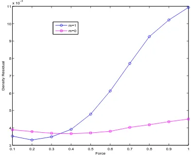
As remarked earlier, the Mach number is dependent on the particle mass, mean flow velocity,

and investigate the variation in number density, measured through

1 Nb

v u u

tN

b X

i=1

(ni−n)2, (49)

where Nb is the number of bins in the fluid region and ni the calculated number density in

bin i. This may be regarded as a measure of compressibility. Results obtained are shown

in Figure 8. With increasing external force, the residual in number density of the unit mass

case grows much faster than in the case of zero mass (for the external force increasing from

0.1 to 1, this compressibility measure increases by 3.10 times form= 1 and only 1.16 times

form = 0). Regarding the variation in divergence of velocity (∇.u), the behaviour is similar.

As the external force changes from 0.1 to 1, the increase in ∇.u is 4.60 times for m= 1 and

only 1.41 times form= 0. The overdamped limit clearly promotes incompressibility.

4.3

Particulate suspensions

A suspended particle of spherical/circular shape can be modelled using a single DPD particle

[15-19,8] or a set of frozen DPD particles [20-23]. The single particle model involves three

groups of DPD parameters: the first group associated with the interactions between

solvent-solvent particles, the second with solvent-solvent-colloidal particles and the third with

colloidal-colloidal particles. They all need be defined in advance; more effort is required for the second

group, particularly for the case of polydispersed suspensions (colloidal particles having a size

distribution). The frozen particle model requires a relatively large number of DPD particles

on the surface to represent a colloidal particle, resulting in systems of larger size for a given

volume fraction. The position and velocity of a colloidal particle are advanced according to

the Newton-Euler equation. The present work is concerned with the modelling of massless

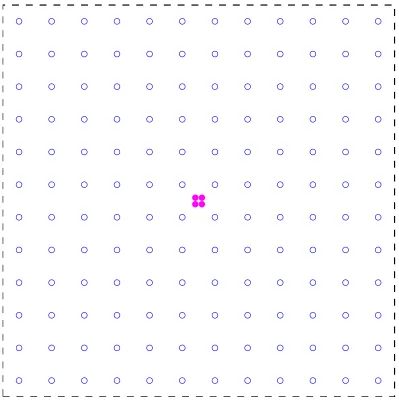
suspended particles (cylinders). We propose to use a set of only three basic DPD particles

(referred to here as “constituent particles”) to represent a colloidal particle, in which they are

connected together via springs(Figure 9a). The stiffness of springs is chosen to be large but

still maintaining the fluctuating motion part of these DPD particles (constituent particles).

Consequently, the motion of a colloidal particle is also updated using DPD equation, which

denote a pair of constituent particles of a colloidal particle. The velocity DPD equations for

the particlesα and β become

N

X

j=1,j6=α

(Fαj,C+Fαj,D+Fαj,R)−H(rαβ−rαβ)

r_αβ

rαβ

= 0, (50)

N

X

j=1,j6=β

(Fβj,C+Fβj,D+Fβj,R) +H(rαβ−rαβ)

rαβ

rαβ

= 0, (51)

where H is the stiffness of springs and rαβ the reference length (the initial length of the

spring). The proposed model only involves DPD parameters of the fluid case and one extra

parameter, namely the stiffness of springs, which can be easily chosen. Constituent particles

of the colloids are basically the same as solvent particles since they are all subject to the

same values of DPD parameters including the thermodynamic temperature. In this regard,

the volume fraction can be simply defined as φ = N0

c/(Ns +Nc0), where Ns is the number

of basic particles used to represent the solvent phase and N0

c the number of basic particles

used to model the colloidal phase.

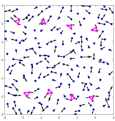
Our computational domain is taken as 6×6. With n= 4, there are 144 free DPD particles

used to represent the fluid phase. An illustration of the spatial configuration of the DPD

system at an instant time is shown in Figure 9b. We employ a shear rate in the range of

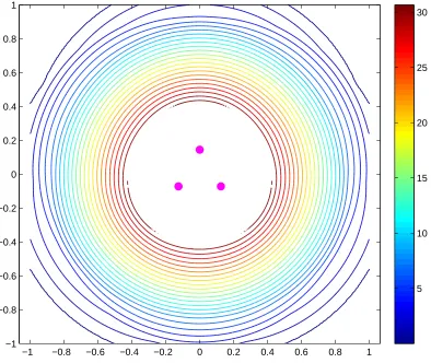
0.25 to 33 and spring stiffness H = 1000. Figure 10 displays the radial component of the

conservative force field generated by three basic particles that are located at the vertices

of an equilateral triangle with rαβ = 0.25. We utilise expression (48) to measure the size

of particles, resulting in a nearly zero size (a < 0.01) for a solvent particle and a ≈ 0.2

for a colloidal particle (Figure 11). We observe that the spring forces on the constituent

particles of the colloidal particle are oscillatory with zero mean and they thus do not make

any contributions to the stress tensor. The self diffusion D is measured by means of mean

squared displacement (MSD)

D= 1

4tlim→∞

d

dth|ri(t)−ri(0)|

2_{i, (52)}

which is calculated in ensemble-average sense for the solvent particle and time-average sense

latter. The self diffusion is seen to reach a stable stage very quickly. In the solvent case, the

MSD curves contain some fluctuations, probably due to the combination of zero mass (i.e.,

no inertial forces) and small particle size. The P´eclet number is defined as P e = ˙γa2_/D,

where ˙γ,a and Dare the shear rate, radius and diffusion coefficient of a suspended particle,

respectively. This number measures the relative importance of dissipative (hydrodynamic

contribution) and random (random contribution) forces.

For 2D dilute suspensions, the relative/reduced viscosity, which is the ratio of the effective

viscosity of the suspension to that of the suspending fluid, has been shown to be [24]

ηr = (1 + 2φ), (53)

whereφis the volume fraction. We employ several sets of colloids: (1,2,3,4,6,8),

correspond-ing to volume fraction in range of 0.0204 to 0.1429. Figure 12 shows good agreement between

the present relative viscosities and those predicted by (53) asφapproaches zero. We observe

a decrease in viscosity with increasing P´eclet number (i.e., shear thinning) for low values of

φ as shown in Figure 13.

5

Concluding remarks

We investigate the behaviour of strongly overdamped DPD systems in modelling the

inter-action between fluid and solid objects. Two iterative numerical schemes are proposed for

solving the resultant sparse DPD system at each time step. With the presence of frozen

particles in wall regions, a relative representation of particle motion with respect to the

centre of mass is a better means to model the flow - in this representation, the artifacts

due to the reaction forces are eliminated. In addition, the inclusion of the physical velocity

constraint of the mass centre into the DPD system significantly enhances the efficiency of the

iterative solving process. Solid objects of circular shape can be modelled using 3 or 4 basic

DPD particles only. Results obtained for flows in periodic arrays of cylinders and particulate

suspensions at a dilute/semi-dilute regime and zero Reynolds number agree well with those

improves the dynamic response of the DPD fluid, allowing creeping flows of complex fluids

(suspension, emulsion, polymer solution, polymer melt, etc.) to be effectively modelled.

Acknowledgement

This work is supported by The Agency for Science, Technology and Research (A*STAR)

through grant #102 164 0145. N. Mai-Duy also would like to thank the Australian Research

Council for an ARC Future Fellowship (FT0990768).

References

1. P.J. Hoogerbrugge, J.M.V.A. Koelman, Simulating microscopic hydrodynamic

phe-nomena with dissipative particle dynamics, Europhysics Letters. 19(3) (1992) 155-160.

2. P. Espa˜nol, P. Warren, Statistical mechanics of dissipative particle dynamics,

Euro-physics Letters. 30(4) (1995) 191-196.

3. P. Espa˜nol, Hydrodynamics from dissipative particle dynamics, Phys. Rev. E. 52

(1995) 1734-1742.

4. R.D. Groot, P.B. Warren, Dissipative particle dynamics: Bridging the gap between

atomistic and mesoscopic simulation, J. Chem. Phys. 107 (1997) 4423.

5. C. Marsh, Theoretical aspect of dissipative particle dynamics (PhD Thesis), University

of Oxford, 1998.

6. D. Pan, N. Phan-Thien, N. Mai-Duy, B.C. Khoo, Numerical investigations on the

compressibility of a DPD fluid, Journal of Computational Physics. 242 (2013)

196-210.

7. X.J. Fan, N. Phan-Thien, S. Chen, X. Wu, T.Y. Ng, Simulating flow of DNA suspension

using dissipative particle dynamics, Phys. Fluids. 18(6) (2006) 063102.

8. N. Mai-Duy, D. Pan, N. Phan-Thien, B.C. Khoo, Dissipative particle dynamics

9. N. Phan-Thien, N. Mai-Duy, D. Pan, B.C. Khoo, Exponential-time differencing schemes

for low-mass DPD systems, Computer Physics Communications. 185(1) (2014)

229-235.

10. N. Mai-Duy, N. Phan-Thien, B.C. Khoo, A numerical study of strongly overdamped

Dissipative Particle Dynamics (DPD) systems, Journal of Computational Physics. 245

(2013) 150-159.

11. N. Phan-Thien, Understanding Viscoelasticity: An Introduction to Rheology, second

Edition, Springer-Verlag, Berlin, 2013.

12. E. Bodewig, Matrix Calculus, North-Holland Publishing, Amsterdam, 1956.

13. N. Phan-Thien, S. Kim, Microstructures in Elastic Media: Principles and

Computa-tional Methods, Oxford University Press, New York, 1994.

14. H. Hashimoto, On the periodic fundamental solutions of the Stokes equations and their

application to viscous flow past a cubic array of spheres, Journal of Fluid Mechanics.

5(2) (1959) 317-328.

15. W. Dzwinel, D.A. Yuen, A two-level, discrete-particle approach for simulating ordered

colloidal structures, Journal of Colloid and Interface Science. 225(1) (2000) 179-190.

16. V. Pryamitsyn, V. Ganesan, A coarse-grained explicit solvent simulation of rheology

of colloidal suspensions, J. Chem. Phys. 122 (2005) 104906.

17. W. Pan, I.V. Pivkin, G.E. Karniadakis, Single-particle hydrodynamics in DPD: A new

formulation, EPL. 84(1) (2008) 10012.

18. W. Pan, B. Caswell, G.E. Karniadakis, Rheology, microstructure and migration in

Brownian colloidal suspensions, Langmuir. 26(1) (2010) 133-142.

19. M. Whittle, K.P. Travis, Dynamic simulations of colloids by core-modified dissipative

particle dynamics, J. Chem. Phys. 132 (2010) 124906.

20. J.M.V.A. Koelman, P.J. Hoogerbrugge, Dynamic simulations of hard-sphere

21. E.S. Boek, P.V. Coveney, H.N.N. Lekkerkerker, P. van der Schoot, Simulating the

rheology of dense colloidal suspensions using dissipative particle dynamics. Phys. Rev.

E. 55(3) (1997) 3124-3133.

22. N.S. Martys, Study of a dissipative particle dynamics based approach for modeling

suspensions, J. Rheol. 49 (2005) 401.

23. S. Chen, N. Phan-Thien, B.C. Khoo BC, X.-J. Fan, Flow around spheres by dissipative

particle dynamics, Phys. Fluids. 18(10) (2006) 103605.

24. J.F. Brady, The Einstein viscosity correction in n dimensions, International Journal of

0 500 1000 1500 2000 2500 10−8

10−7 10−6 10−5 10−4 10−3 10−2 10−1 100 101

Number of iterations

Convergence measure

Scheme 1 Scheme 2

Figure 2: Couette flow: Scheme 2 converges much faster than Scheme 1. Given a tolerance of 10−7_{, the Picard algorithm typically requires about 2100 and 450 iterations for Scheme 1}

−5 −4 −3 −2 −1 0 1 2 3 4 5 −10

−8 −6 −4 −2 0 2 4 6 8 10

n u_x

u_y

Figure 3: Couette flow, Lx×Ly = 10×10, ∆t = 0.01: variations of number density and

−5 −4 −3 −2 −1 0 1 2 3 4 5 −10

−8 −6 −4 −2 0 2 4 6 8 10

y

u x

−5 −4 −3 −2 −1 0 1 2 3 4 5

−10 −8 −6 −4 −2 0 2 4 6 8 10

y

u x

−1 −0.8 −0.6 −0.4 −0.2 0 0.2 0.4 0.6 0.8 1 −1

−0.8 −0.6 −0.4 −0.2 0 0.2 0.4 0.6 0.8 1

5 10 15 20 25 30 35 40 45 50 55

−3 −2 −1 0 1 2 3

−2.5 −2 −1.5 −1 −0.5 0 0.5 1 1.5 2 2.5

0 1 2 3 4 5 6

0 1 2 3 4 5 6 7 8 9 0

20 40 60 80 100 120 140 160 180

Mean velocity

Drag force

Hasimoto, 1959 Present DPD

0.1 0.2 0.3 0.4 0.5 0.6 0.7 0.8 0.9 1 3

4 5 6 7 8 9 10 11x 10

−3

Force

Density Residual

m=1 m=0

-3 -2 -1 0 1 2 3 -3

-2 -1 0 1 2 3

−1 −0.8 −0.6 −0.4 −0.2 0 0.2 0.4 0.6 0.8 1 −1

−0.8 −0.6 −0.4 −0.2 0 0.2 0.4 0.6 0.8 1

5 10 15 20 25 30

0 0.1 0.2 0.3 0.4 0.5 0.6 0.7 0.8 0.9 1 0

0.2 0.4 0.6 0.8 1 1.2 1.4

Distance

RDF

0 0.1 0.2 0.3 0.4 0.5 0.6 0.7 0.8 0.9 1 0

0.5 1 1.5

Distance

RDF

−0.021 0 0.02 0.04 0.06 0.08 0.1 0.12 0.14 0.16 1.05

1.1 1.15 1.2 1.25 1.3 1.35 1.4

Volume fraction

Relative viscosity

DPD Theories

10−1 100 101 102 2.6

2.7 2.8 2.9 3 3.1 3.2 3.3 3.4 3.5 3.6

Pe

Viscosity

φ=0.02

φ=0.06

φ=0.11

φ=0.14