Thesis by
Christopher David White
In Partial Fulfillment of the Requirements for the Degree of
Doctor of Philosophy
CALIFORNIA INSTITUTE OF TECHNOLOGY Pasadena, California
2019
c 2019
Christopher David White ORCID: 0000-0002-8372-2492
ACKNOWLEDGEMENTS
ABSTRACT
This thesis describes two studies of the dynamics of many-body quantum sys-tems with extensive numerical support.
In Part I we first give a new algorithm for simulating the dynamics of one-dimensional systems that thermalize (that is, come to local thermal equilib-rium). The core of this algorithm is a new truncation for matrix product operators, which reproduces local properties faithfully without reproducing non-local properties (e.g. the information required for OTOCs). To the ex-tent that the dynamics depends only on local operators, timesteps interleaved with this truncation will reproduce that dynamics.
We then apply this to algorithm to Floquet systems: first to clean, non-integrable systems with a high-frequency drive, where we find that the system is well-described by a natural diffusive phenomenology; and then to disordered systems with low-frequency drive, which display diffusion—not subdiffusion— at appreciable disorder strengths.
PUBLISHED CONTENT AND CONTRIBUTIONS
This thesis contains material from:
White, C.D., Zaletel, M.,, Mong, R.S.K., and Refael, G. “Quantum Dynamics of Thermalizing Systems.” Phys. Rev. B 97, 035127 (2018). DOI: 10.1103/phys-revb.97.035127.
CDW constructed the algorithm used, wrote the algorithm-specific code, con-structed the benchmarking protocol, carried out the simulations, and performed the analysis.
Ye, B., Machado, F., White, C.D., Mong, R.S.K., and Yao, N. “Emergent hydrody-namics in Floquet quantum systems”. arXiv:1902.01859.
CDW participated in the conception of the project and the analysis of the re-sults (in particular the framing in terms of hydrodynamics). In addition, the project used CDW’s algorithm-specific code.
Yunger Halpern, N., White, C.D., Gopalakrishnan, S., and Refael, G. “Quantum engine based on many-body localization”. Phys. Rev. B. 99, 024203. DOI: 10.1103/physrevb.99.024203
TABLE OF CONTENTS
Acknowledgements . . . iii
Abstract . . . iv
Published Content and Contributions . . . v
Table of Contents . . . vi
Introduction . . . ix
Chapter I: Background: MBL and MPS . . . 1
1.1 Many body localization . . . 1
1.1.1 Many-body localization in perturbation theory . . . 1
1.1.2 Long-time memory in MBL systems . . . 5
1.1.3 Level spacing . . . 7
1.1.4 Local dynamics at finite time . . . 10
1.2 Matrix product states . . . 10
1.2.1 Graphical notation for tensors and tensor contractions 14 1.2.2 Expectation values and correlations in MPSs . . . 15
1.2.3 Canonical forms and orthogonality centers . . . 16
1.3 Dynamics and matrix product states . . . 20
1.4 Matrix product operators . . . 21
1.4.1 MPO representation of an exponential interaction . . . 22
1.4.2 MPO representation of a power-law Hamiltonian . . . . 23
1.4.3 MPDOs . . . 24
1.4.4 Matrix product density operator representations of Gibbs states . . . 26
1.5 Some essentials of quantum thermodynamics . . . 26
I Thermalizing systems and matrix product density
operators
28
Chapter II: Simulating quantum dynamics of thermalizing systems . . 292.1 Background and intuition . . . 30
2.1.1 Background: matrix product state methods . . . 30
2.1.2 Intuition: thermalization and computation . . . 33
2.2 Method: truncation of MPDOs . . . 36
2.2.1 Setting, notation, and tools . . . 37
2.2.2 Re-writing the MPDO to expose properties whose preser-vation we guarantee . . . 39
2.2.3 Modifying the MPDO . . . 41
2.2.4 Preservation of l-site operators . . . 44
2.3 Results . . . 46
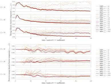
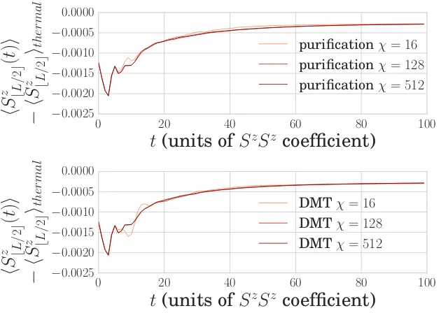
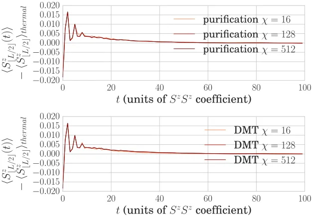
2.3.2 Application: pure-state evolution . . . 47
2.3.3 Application: mixed-state evolution (near equilibrium) . 52 2.3.4 Application: mixed-state evolution (far from equilibrium) 52 2.4 Conclusion . . . 55
Chapter III: Heating, prethermalization, and hydrodynamics in a high-frequency Floquet system . . . 59
3.1 Model and Floquet phenomenology . . . 60
3.2 Benchmarking DMT . . . 65
3.2.1 Benchmarking Krylov subspace dynamics . . . 65
3.2.2 DMT and Krylov . . . 66
3.2.3 Entropy in DMT . . . 69
3.2.4 Effect of Trotter step size on DMT numerics . . . 69
3.3 Analysis and results . . . 71
3.3.1 Approach to Gibbs Ensemble . . . 73
3.3.2 Heating . . . 77
3.3.3 Extracting diffusion coefficients of a spatially uniform, static Hamiltonian . . . 78
3.3.4 Classical diffusion equation . . . 82
3.3.5 Hydrodynamics in large spin chains . . . 86
3.4 Discussion . . . 86
Chapter IV: Hydrodynamics in a disordered low-frequency Floquet system 88 4.1 Model . . . 89
4.2 Method . . . 90
4.2.1 Convergence testing . . . 91
4.2.2 Comparison with exact simulations . . . 93
4.2.3 Quantity of interest . . . 95
4.2.4 Disorder averaging . . . 96
4.3 Results . . . 97
4.4 Discussion . . . 99
II MBL-mobile: Many-body-localized engine
101
Chapter V: MBL and thermodynamic engines . . . 102Chapter VI: The MBL-Mobile in its adiabatic limit . . . 105
6.1 Qubit toy model for the mesoscale engine . . . 105
6.2 Set-up for the mesoscale MBL engine . . . 107
6.3 Notation and definitions: . . . 110
6.4 Quantitative analysis of the adiabatic mesoscale engine: some easy limits . . . 111
6.5 Quantitative analysis of the adiabatic mesoscale engine: a more detailed calculation . . . 113
6.5.1 Partial-swap model of thermalization . . . 113
6.5.2 Average heat hQ2i absorbed during stroke 2 . . . 114
6.5.3 Average heat hQ4i absorbed during stroke 4 . . . 116
6.5.5 Efficiency ηMBL in the adiabatic approximation . . . 120
6.6 MBL engine in the thermodynamic limit . . . 121
6.7 Numerical simulations . . . 125
6.7.1 Hamiltonian . . . 125
6.7.2 Scaling factor . . . 126
6.7.3 Representing states and Hamiltonians . . . 129
6.7.4 Strokes 1 and 3: tuning . . . 129
6.7.5 Stroke 2: Thermalization with the cold bath . . . 130
6.7.6 Results . . . 131
Chapter VII: The MBL-Mobile at finite speed . . . 133
7.1 Diabatic corrections . . . 133
7.1.1 Fractional-Landau-Zener transitions . . . 134
7.1.2 Landau-Zener transitions . . . 135
7.1.3 APT transitions . . . 136
7.2 Numerical simulations . . . 137
7.2.1 Simulating finite-time tuning . . . 138
7.2.2 Enlightenment from numerical methods . . . 139
7.3 Precluding communication between subengines . . . 140
7.4 Lower bound on the cycle time from cold thermalization . . . . 141
Chapter VIII: Racing the MBL-mobile . . . 144
8.1 Comparisons with competitor Otto engines . . . 144
8.1.1 Comparison with bandwidth engine . . . 144
8.1.2 Comparison with MBL engine tuned between same-strength disorder realizations . . . 145
8.1.3 Quantum-dot engine . . . 147
8.1.4 Anderson-localized engine . . . 147
8.2 Order-of-magnitude estimates . . . 148
8.3 Outlook . . . 149
INTRODUCTION
Numerical methods for many-body quantum systems go back to the earliest days of electronic computers. The physicists of Los Alamos during World War II relied heavily on numerical simulations; the first calculations were done by human “computers” or with mechanical calculators,1 but soon after the war they began using ENIAC, the first programmable electronic computer [84]. We need simulations because the phenomena we study are complex. This was certainly the case for the pioneers of computational physics, simulating weapons physics at Los Alamos, and it is the case for us now. We may have a microscopic Hamiltonian, but analytically solving the Schr¨odinger equation with that Hamiltonian is out of the question, and tightly-controlled approx-imations are frequently unavailable. So we are forced to rely on heuristic approximations justified by physical arguments. But these approximations need to be checked: do they describe the model’s behaviour well? At the very least, do they describe some essential phenomenon at work in the system? Nu-merical simulations of a model catch hidden assumptions and subtle mistakes in your physical arguments—and they suggest further approximations to make and phenomena to investigate. (The work of Part II of this thesis proceeded in exactly this fashion, as an ongoing three-part conversation between physical argument, careful analytical work, and numerical simulation.)
But numerical methods are not simply devices for checking your intuitions and arguments. Developing anew numerical method and teasing out a characteri-zation of where it succeeds, where it fails, and why it succeeds or fails provides important insight into the physics of the systems that method simulates Take the history of thedensity matrix renormalization group(DMRG) and thematrix product state(MPS).2 Steve White developed the method in 1993 [226, 227] as an extension of Wilson’s numerical renormalization group (NRG) [230], and it quickly saw wide application [82, 100, 127, 180], not only for computing ground states but also for simulating low-energy dynamics. Meanwhile, in 1995, Ostlund and Rommer [248] showed that “infinite-system” DMRG could be formulated in terms of matrix product states, which had existed for some time, e.g. as a mechanism for writing down the ground
1The Los Alamos physicists required numerical stability from their algorithms because
dust caused frequent errors.
state of the AKLT Hamiltonian [9, 10, 59], and in 1999 Takasaki et al. [203] showed that “finite-system” DMRG is precisely a variational procedure, which iteratively minimizes the energy over the manifold of matrix product states. The notion of truncation was crucial to the practical developments. Matrix product states offer not only a compact representation of low-entanglement states, but also an obvious procedure for “lossy compression”—for optimally approximating one matrix product state by another that requires less memory and computation time to store and use.
The growing understanding that ground states of gapped Hamiltonians have efficient matrix product state representations (in particular the work of Hast-ings, e.g. [86]) gave physicists the confidence to use DMRG as, essentially, a black-box method. Since most translation-invariant local Hamiltonians are gapped (see [131] for a recent proof) and ground states of gapped Hamilto-nians have efficient matrix product representations, one expects DMRG to reliably find the ground state of an arbitrarily-chosen Hamiltonian. And DMRG is generally self-diagnosing: even if it does fail, you can tell by checking convergence in the simulation parameters, without having to com-pare to an exact result, or argue without empirical evidence that it should give the right answer.3 Even if you are not a specialist, you can choose from a number of carefully-optimized, well-engineered MPS implementations, e.g. ITensor [1] or TeNPy3 [87], and expect that either DMRG will work or you will see clear evidence that it fails. The long list of papers using ITensor (http://itensor.org/docs.CGI?page=papers) testifies to the impact of this
development.
But that understanding also led to a number of analytical results, notably Xie Chen and friends’ classification of bosonic symmetry protected topological phases (SPTs) [36]; cf Pollmann and friends’ [169, 170]. [170] is particularly close to the spirit of this thesis: in it, Pollmann and his collaborators ask how symmetry operations act on the vector space in which the entanglement spectrum of an MPS in mixed canonical form lives. They find that the decomposition of that vector space into irreducible projective representations of the symmetry group strongly constrains the entanglement spectrum.
3A few of DMRG’s failure modes, notably difficulty capturing rare long-range
And DMRG also gave rise to a variety of numerical methods for time evolution, notably TEBD [213, 214, 228]. (I discuss TEBD in some detail in Sec. 1.3, and give an opinionated discussion of a variety of MPS-based time evolution methods in Sec.2.1.1.) These numerical methods in turn shed light on one of the fundamental questions of computational physics—what physical processes can one efficiently simulate on a classical computer?—by carving out a set of quantum problems—namely those that generate little entanglement—that can be efficiently simulated. This question in turn is intimately related to the
extended Church-Turing thesis. Other work along these lines includes the Gottesman-Knill theorem [73], which shows that computations involving only Clifford gates are efficiently simulable on classical computers.
A feedback loop between development and characterization of numerical meth-ods, on the one hand, and analytical work of varying degrees of rigor on the other, is clearly a fruitful way to do research: it leads to both practical nu-merical methods and to a deeper analytical understanding of the phenomena we started out trying to simulate.
Because thermalizing systems generate entanglement quickly, TEBD is of lim-ited utility, and numerical studies were for some time restricted to exact di-agonalization (e.g. [115]), with occasional forays into special-purpose MPS or matrix-product operator (MPO) calculations (e.g. [113]). But in the last few years, three methods—TDVP [133], CTWA [233, 234], and my own density matrix truncation, or DMT—have density matrix truncation come into use; they promise to shed light on the physics of thermalizing systems. This thesis sits in the tradition I have sketched of using both sides of this feedback loop to advance the discipline.
I present necessary background in Chapter 1. The later chapters assume some basic knowledge of many-body localization, matrix product states, and algo-rithms for time evolution. Chapter 1 communicates that knowledge. I aim more for intuition than rigor. Nothing in 1 is original; most of the contents are ambient cultural knowledge, so I include few citations.
Part I describes DMT and the physics we can use it to study. DMT is a new describe a new algorithm for approximating matrix product representations of density matrices that takes advantage of our understanding of thermalization. It succeeds at simulating previously unsimulable systems, and its convergence properties already prompt interesting insights into those systems.
In Ch. 2, we argue that truncating MPDOs in such a way that the expectation values of the conserved quantities of some thermalizing Hamiltonian do not change should not change the long-time dynamics of that Hamiltonian. We construct a truncation procedure that does this, and find that it does indeed capture the long-time dynamics of a fruit-fly thermalizing Hamiltonian. In Ch. 3 we apply DMT to a high-frequency Floquet system. We find that it accurately captures not only the system’s hydrodynamics but also the Floquet heating process; the degree to which it does this illuminates the details of that process. We also find that the long-time prethermal dynamics of the system are well-described by a phenomenological diffusion equation In Ch. 4, we apply DMT to a low-frequency disordered Floquet system, and find that even for substantial disorder its hydrodynamics are diffusive. We also comment on some subtleties in evaluating DMT’s accuracy, and the degree to which it is self-diagnosing.
relatively straightforward adiabatic limit (Ch. 6); we then analyze finite-speed effects (Ch. 7), and compare it to competitor engines (Ch. 8).
C h a p t e r 1
BACKGROUND: MBL AND MPS
1.1 Many body localization
1.1.1 Many-body localization in perturbation theory
Consider a random paramagnet—a system with Hamiltonian Hrpara =
X
hzjσ z
j , (1.1)
where thehz
j are drawn independently from the uniform distribution on [−h, h].
A system governed by this state has “perfect memory” in the sense that if it starts out in some product of σz
j eigenstates, say
|0xC0FFEEi=|↑↑↓↓↓↓↓↓↑↑↑↑↑↑↑↑↑↑↑↓↑↑↑↓i , (1.2) it will remain in that state forever: e−iHt|0xC0FFEEi = |0xC0FFEEi, up to a
phase, for all t. In terms of operators d
dthσ
z
ji=−ih[Hrpara, σ z
j]i= 0 . (1.3)
Indeed [Hrpara, σjz] = 0: the σzj are conserved quantities of the Hamiltonian
Hrpara.
Now suppose we change the Hamiltonian. Suppose in particular that we add a nearest neighbor interaction:
HRFH =Hrpara+t
X
j
[σx jσ
x j+1+σ
y jσ
x
j+1] + ∆
X
j
σz jσ
z j+1] =tX
j
[σxjσ x j+1+σ
y jσ
x
j+1] + ∆
X
j
σjzσ z j+1+
X
j
hzjσ z j ,
(1.4)
hz
j still random in [−h, h]. (I choose this Hamiltonian with malice aforethought.
Since the work of Pal and Huse [160] this Hamiltonian, called the random-field Heisenberg Hamiltonian, has served as the fruit-fly model for the study of many body localization: see inter alia multa [246].) Then
i.e. theσz
j are no longer conserved quantities. Disaster!
But if h is large, the σz
j are almost conserved. First, take ∆ = 0 and add
h6= 0. Then the Hamiltonian is H& =t
X
j
[σjxσ x j+1+σ
y jσ
x j+1] +
X
j
hzjσ z
j . (1.6)
On Jordan-Wigner transformation this is the single-particle Hamiltonian H& = 2t
X
j
[c†jcj+1+ h.c.] +
X
j
hzjnj . (1.7)
I’m going to take as read the fact that this Hamiltonian displays Anderson localization, so its single-particle eigenstates are localized with some local-ization length, call it ζ.
To put that statement about localized single-particle eigenstates in a more useful form, write ˜nj for the occupation number operator of the eigenstate
centered at site j, and write τz
&j = 2˜nj. (Similarly Jordan-Wigner transform
˜
c†∼τ+.) τz
&j is called an (Anderson) l-bit. Then
H& =
X
j
h0jτz
&j , (1.8)
where the h0
j are the eigenenergies of the single-particle eigenstates. There is
some unitary U& (namely the unitary diagonalizing H&) such that U&†τz
&jU& =σz (1.9)
and U&†τ&+jU& = σ+, etc. Since the single-particle eigenstates are localized with localization length ζ,
τz
&j ∼σjz+ X
kl
Rjkle−(|k−j|+|j−l|)/ζσ+
kσ
−
l (1.10)
for some appropriate random Rjkl.
How do interactions change this picture? Add an interaction term V =
P
jσjzσjz+1, for
HRFH =H&+V =
X
~σj ·~σj+1+
X
j
We would hope to treat this as a perturbation. We can only do so if
Dhαα|V−|Dαβi
1. (1.12)
To estimate this, suppose two states|αi,|βidiffer on a subsystem of diameter l: that is,
|αihβ|=τ&+a1. . . τ&+anτ&−b1. . . τ&−bm , (1.13) where the sites a1, . . . an, b1, . . . , bm are all in a subsysteml. Then
hβ|σz jσ
z
j+1|αi= tr
σz jσ
z
j+1|αi hβ|
= trσz jσ
z
j+1τ&+a1. . . τ
+ &anτ
− &b1. . . τ
− &bm
= trh(U&†σz
jσzj+1U&)σ+a1. . . σ
+
anσ
−
b1. . . σ
−
bm i
.
(1.14)
What is the operator content of this strange construction U†σz
jσjz+1U? We know that conjugation byU maps
U&σjzU
† &∼ 1 ζσ z j + X kl
Rjkle−(|k−j|+|j−l|)/ζσk+σl− (1.15)
with Rklj ∼ζ−1 random, so it is reasonable to suppose thatU†σz
jσjz+1U is U†σz
jσ z j+1U =
X
~ ν
Rj~ν2−2`[~ν]e−`[~ν]/ζσ~ν , (1.16)
whereRj~ν ∼ 1ζ,~ν =ν1ν2ν3. . . νl, νj ∈0. . .3 label Pauli stringsσ~ν, we take each
~ν to have at least oneνj 6= 0, and`[~ν] is the natural notion of the diameter of
the Pauli string σ~ν
`[~ν]≡max{j :νj 6= 0} −min{j :νj 6= 0}. (1.17)
The factor of 2−2`[~ν] ensures normalization. Then hβ|σz
jσ z
j+1|αi= tr
(U†σz jσ
z
j+1U)σa+1. . . σ
+
anσ
−
b1. . . σ
−
bm
∼2−l/2e−l/ζ . (1.18)
The energy difference is typically not less than the spacing of levels on l sites:
So our condition forV to act perturbatively is that for most α, β
1
Dhαα|V−|Dββi
∼el(ln 2−ζ
−1)
(1.20)
or equivalently that the bare model H& have localization length
ζ−1 >ln 2. (1.21)
(This is a heuristic sketch of certain elements of de Roeck et al.’s “avalanche picture”; see also [5, 49, 145, 171, 206, 207]. The chief element I have not treated is the possibility—near certainty, in fact—that some regions will be resonant in the sense in the sense that the condition (1.20) is not satisfied; de Roeck and friends give an RG-like scheme for determining whether these “resonant regions” destabilize the Anderson-localized system.)
If you carry this diagonalization out in full you will find a unitaryU such that τz
j =U τ&zjU†=U U&σjzU
† &U
†
& is a conserved quantity of HRFH:
[HRFH, τjz] = 0 . (1.22)
Based on the condition (1.20) and the expectation that higher-order terms will scale as
[nth-order term] ∼el(ln 2−ζ−1)n , (1.23) one expects these l-bits to have the form localization length
τjz ∼U
†
U&†σzjU&U ∼ 1 ξσ
z
j +
X
kl
Rjkle−(|k−j|+|j−l|)/ξσ+kσ−l (1.24)
where
ξ= (ln 2−ζ−1)−1 . (1.25) (Again this is morally consistent with the results of the avalanche picture, but they run this quantity through an RG scheme.) We have therefore constructed extensively many local integrals of motion. These are l-bits in the usual sense [34, 92].
Figure 1.1: Left: Notional density of states (hence entropy density) for a disor-dered many-body system. Right: Notional phase diagram, per (1.21). Com-pare the phase diagram found in [146] for the isotropic random-field Heisenberg model.
1. Systems with larger onsite Hilbert spaces, from the prosaic (spin-3/2 sites) to the exotic (SYK puddles), will require larger disorder to localize (if they localize at all: constructing this Anderson route to MBL will require creativity).
2. Since for real systems the entropy density is a function of energy density, the condition (1.21) (as well as the more sophisticated treatments of de Roeck et al.) na¨ıvely predict a mobility edge. See Fig. 1.1. But de Roeck et al. argue in [48] that a mobility edge is impossible, in the sense that it will destabilize localized states at lower energies. Per this arguement, interacting systems must be fully MBL (no mobility edge) or not MBL at all. On the other hand, numerics (e.g. [146]) consistently show a mobility edge consistent with the na¨ıve prediction of (1.21)). My own belief is that that the mobility edge exists, but this will require a great deal of work to sort out.
In addition, the full avalanche picture predicts that MBL cannot exist ind≥2 dimensions. You can already glimpse how this comes about: if you construct a perturbative scaling in some lengthl based on (1.20), the level spacing shrinks exponentially in ld, while the matrix element only shrinks exponentially in l.
So in d≥2, couplings are always resonant at sufficiently long length scales.
1.1.2 Long-time memory in MBL systems
We started with a simple question about a system’s memory: supposing I started out in state |0xCOFFEEi, does the system remain recognizably in that state? If the system is a random paramagnet, it obviously does: [H, σz
If the system is goveerned by a random-field Heisenberg model, the situation is more complicated. Then [HRFH, σjz]6= 0, but as we have just seen there are
operators τz
j not so different from σzj that are conserved.
Instead of worrying about the instantaneous decay d dtσ
z
j =−i[HRFH, σjz], attack
the long-time limit directly. Work in the fermion picture, withnj = 12(σjz+ 1).
If Eα are the eigenenergies of HRFH, then lim
t→∞nj(t) = limt7→∞
X
αβ
e−i(Eα−Eβ)t|αi hα|n
j|βi hβ| . (1.26)
This is strongly oscillatory, so the outcome could depend strongly on when exactly we take the measurement. Clearer would be to start a measurement after some timet0 and let the measurement go on for some very long timeT:
1
T t0,Tlim→∞ Z t0+T
t0
nj(t) = X
αβ
|αihα|nj|βihβ|
1
T t0,Tlim→∞ Z t0+T
t0
e−i(Eα−Eβ)t
=X
α
tr [|αihα|nj] .
(1.27)
The eigenstates|αiare specified by l-bit occupations, e.g. |αi=|10011101. . .i, so eigenstate projections are
|αihα|=Y
j∈α
˜ nj
Y
k6∈α
˜
nk , (1.28)
where j ∈α indicates that l-bitj is occupied in state|αi, and I write
˜ nj =
1 2(τ
z
j + 1)∼
1 ξnj+
X
jk
e−ξ|j−k|
c†jck+. . . (1.29)
for the occupation operator of the l-bit centered atj. That occupation operator looks like
˜ nj ∼
1 ξn z j + X kl
Rjkle−(|k−j|+|j−l|)/ξc†
kcl . (1.30)
Then 1
T t0,Tlim→∞ Z t0+T
t0
nj(t) = X
α
tr
" Y
k∈α
˜ nk
Y
k06∈α ˜ nk0nj
#
Since
nj ∼
1
ξn˜j + [multiple l-bit flips with small coeff’s], (1.32) this is roughly
1
T t0,Tlim→∞ Z t0+T
t0
nj(t) =
1 ξ
X
α
tr
" Y
k∈α
˜ nk
Y
k06∈α ˜ nk0nj
#
|αihα| 'n˜j :
(1.33)
the long-time expectation value is given by the nearest l-bit.
1.1.3 Level spacing
This long-time memory, while conceptually satisfying, is too blunt a knife either for diagnostics or for detailed considerations of dynamics. Level spacing statistics—in particular, the distribution of gaps between nearest-in-energy eigenstates, is a much finer tool: it is a standard diagnostic of thermalization and localization, and we will use it extensively in Part II.
To understand the level-spacing statistics of a disordered Hamiltonian, think once again about a random-field Heisenberg model, this time on a system of size L with closed boundaries. To estimate the distribution of smallest gaps, start in an eigenbasis of the underlying Anderson-localized system. Once again, we’ll proceed by perturbation theory, but along a different route. Suppose for the moment that the system is many-body localized, and take two eigenstates |αi,|α+ 1i of H& with energies E&α, E&α+1. Nearest-in-energy eigenstates will differ on most of the system’s Anderson l-bits, so on the one hand
δ&≡E&α+1−E&α ∼2−L, (1.34)
and on the other
λ≡ hα|σjzσ z
j+1|α+ 1i ∼2
−L/2e−L/ζ
. (1.35)
We can then write an effective two-level Hamiltonian on these two levels
H =
"
δ& λ λ −δ&
#
Figure 1.2: Heuristic derivation of level-spacing distribution
The eigenvalues of (1.36) are
E =±h
q
δ2
&+λ2 , (1.37)
so the gap is δ=pδ2 &+λ2.
What is probability distribution of gaps δ? Suppose now that the system is MBL, and indeed far from the transition. Both δ& and λ are uniformly distributed on their respective scales, but λδ&: this is the condition (1.20) for the system to be MBL. To see the distribution ofδ, Imagine plottingδ&, λ in a plane (cf Fig. 1.2). For small δ (i.e. δ .λ) the ensemble-averaged level-spacing distribution is
lim
s→0p(δ)dδ∼δ dδ, δ.λ; (1.38) for δ&λ,
p(δ)dδ ∼const.×dδ, λ .δ.h . (1.39) We are therefore unlikely to see gaps smaller than
λ∼2−L/2e−L/ζ . (1.40)
This logic was for gaps δ 2−L. If the gap is larger, δ ∼ 2−L, the reasoning
above still holds—but δ ∼ δ&, and you must concern yourself with the fact that δ& is not uniform. Take two Anderson levels separated by a gap δ&0 . As δ0
& increases, the two levels with which you have concerned yourself are increasingly unlikely to be nearest-neighbors in specrum: there is likely to be a level in between. Taking this into account, one finds that
where µ = 2L is [average Anderson gap]−1. (In Part II, we will frequently concern ourselves with the detail that the rate µ can vary with energy.) So
p(δ)∼
δ δ .λ
µe−δ δ &λ . (1.42)
It is convenient to have a single parameter to characterize this level repulsion. Your first thought is probably to compute moments of the level-spacing dis-tribution (1.42), but none are suitable: hsi = 1 by construction, and higher moments capture the large-s behavior—not the small-s behavior we’re after. Moreover, estimating the level-spacing distribution requires that finicky nor-malization by the density of states.
Instead, it is conventional to use the so-called gap ratio, frequently called the r-parameter. Given two adjacent level spacingsδj =Ej−Ej−1 andEj+1−Ej,
the gap ratio is
rj =
min (δj, δj+1) max (δj, δj+1)
. (1.43)
The gap ratio characterizes the distribution (1.42), so one should average it both over levels of a single Hamiltonian and over Hamiltonians drawn from whatever ensemble you’re studying.
To get some intuition, consider two limiting cases:
• If the system has an exact two-fold degeneracy (e.g. a global spin-flip) then small gaps are frequent, and
min (δj, δj+1) = 0 max (δj, δj+1)6= 0
(1.44)
for
r= 0. (1.45)
• If the eigenvalues are uniformly spaced then small gaps never show up, and
δj =δj+1 (1.46)
so min (δj, δj+1) = max (δj, δj+1) for
1.1.4 Local dynamics at finite time
We can use the level spacing to tease out details of the intermediate-time dy-namics of MBL systems. Think about the evolution of the Heisenberg operator
σz(t). (1.48)
How many sites does the operator touch? That is, how many sites in the initial state does hσz
j(t)i depend on? This is essentially a time-dependent correlation
length: σz
j(t) and σkz(t) will be correlated to the extent that they depend on
the same sites in the initial state.
To compute this correlation function, note that on a timescale tthe dynamics is insensitive to gaps smaller thant−1: if two levels are separated by a smaller gap they will not have had time to dephase. All levels differing on a subsystem of diameter
l(t)∼ lnt
ln 2−ζ−1 ∼ξlnt, (1.49) then, will have had time to dephase, but many levels separated on longer length scales will not—so σz(t) will have supportl(t)∼ξlnt. (Cf [109, 158].)
This in turn predicts that the entanglement entropy should be
S ∼ls∝lnt, (1.50)
where s is an entropy density; this is exactly what MPS simulations see [16, 194].
This reasoning will make a reappearance in Chs. 6 and 7.
1.2 Matrix product states
So take an arbitrary state
|ψi= X
s1...sN
ψs1...sN|s1. . . sNi (1.51)
with short-range correlations on anN-site system with closed boundary condi-tions. We want a “computationally efficient” representation for the state—that is, an approximation to|ψi such that that
1. the representation requires little memory, as long as |ψi has a short correlation length;
2. typical operations require little time (polynomial in system size), again as long as |ψi has a short correlation length;
3. the representation can “expand” to represent even states that are not short-range entangled.
Such a representation exists: the matrix product stateorMPS. The stan-dard reference on matrix product states is the review of Schollw¨ock [187] . The field has seen many new developments since that review (some described in this thesis), but none have achieved the widespread acceptance of DMRG or TEBD have. For a very different perspective, see the book of Xie Chen et al. [242] .
To get some intuition for matrix product states work, start with a Schmidt decomposition. Imagine cutting the state in two at some bond l (that is, the bond to the right side of site l). One slightly roundabout way to find the reduced density matrix of the left part of the system is to take the tensor ψs1...sN of Eq. (1.51), group indices to turn it into a matrix,
1 and do a
singular value decomposition (SVD) ψ(s1...sl)(sl+1...sN)=
X
α
U(s1...sl)αsαV(sl+1...sN). (1.52)
This gives
|ψi=X
α
|xLαisα|xRαi (1.53) 1In this case, “grouping indices” is exactly thereshapeoperation in NumPy or Julia.
with
|xLαi= X
s1...sl
U(s1...sl)α|s1. . . sli
|xRαi= X
sl+1...sN
V(sl+1...sN)α|sl+1. . . sNi
(1.54)
Since U, V are isometries
hxLα|xRβi=hxLα|xRβi=δαβ . (1.55)
(Eq. (1.53) is therefore a Schmidt decomposition.) The reduced density ma-trices left and right of bond l are then immediately
ρL= X
α
s2α|xLαihxLα|
ρR= X
α
s2
α|xRαihxRα| .
(1.56)
So the singular valuessαare (the square roots of the) eigenvalues of the density
matrices ρ{L,R}, and entirely specify the state’s entanglement properties: the
2nd R´enyi and von Neumann entanglement entropies, for example, are S2 =
X
α
s4α
SN = X
α
2s2αlgsα .
(1.57)
If the state has low entanglement entropy at bond l, it should require only a few Schmidt vectors to capture—that is, we should be able to write a pretty good approximation by truncating the sum in Eq. (1.53)
If we follow that line of attack, we’re still faced with the problem of representing the states |x{L,R}αi. What we require is a generalization of Eq. (1.53) that in
some sense offers Schmidt decompositions at every bond simultaneously. A matrix product state offers exactly this property. It consists of a decom-position of the tensor ψs1...sN into a product of matrices (hence the name)
ψs1...sN =A
s1
1 As22. . . A
sN
N (1.58)
where each of theAsj
j is a matrix of dimension χ×χ for someχ not too large
(except for As1
1 and A
sN
the bond dimension of the MPS; it controls the computational properties and the entanglement of the MPS. The state is
|ψi= X
s1...sN
As1
1 A
s2
2 . . . A
sN
N |s1. . . sNi (1.59)
(relabeling α 7→α1—in the future such relabelings will be silent) for ψs1(s2...sN)=A
s1
αrαVα(s2...sN) . (1.60)
The index α1 has dimension χ1 given by the rank of the d ×dN−1 matrix ψs1(s2...sN). Now apply roughly the same process to rV: regroup indices so
that it is a (χ1d)×dN−2 and perform an SVD
rαV(α1s2)(s3...sN)=U(α1s2)α2rα2Vα2(s3...sN) . (1.61)
Identify
As2
α1α2 =U(α1s2)α2 (1.62)
for
ψs1s2...sN = X
α1α2
As1 α1A
s2
α1α2rα2Vα2(s3...sN). (1.63)
The index α2 has dimension χ2 given by the rank of the χ1d×dN−1 matrix rαV(α1s2)(s3...sN) Proceed in this way until you find (after doing N −1 SVDs)
ψs1s2...sN =
X
α1α2...αN−1
As1 α1A
s2
α1α2. . . A sN−1
αN−2αN−1VαN−1sN) ; (1.64)
call VαN−1sN) ≡A
sN
αN−1, so
ψs1s2...sN =
X
α1α2...αN−1
As1 α1A
s2
α1α2. . . A sN−1 αN−2αN−1A
sN
αN−1 (1.65)
—this is exactly the form required for Eq. (1.59).
We can bound the bond dimension inductively. χ1 is the rank of a d×dN−1 matrix, so
χ1 ≤d, χ1 ≤dN−1 . (1.66) χ2 is the rank of a (χ1d)×dN−2 matrix, so
Proceeding in this way
χn≤dn, χn ≤dN−n, (1.68)
and in general
χn≤dbn/2c . (1.69)
In fact one rarely constructs an MPS in this way. The utility of MPSs is in the fact that they are efficient representations of states too large to represent otherwise. If the system size is small enough that one can store the whole coefficient tensor ψs1...sN you are almost certainly better off working with the
exact state in an ordinary representation. But the fact that all states can be represented exactly is useful. By taking large bond dimensions, one can perform exact simulations and use them to check your low-bond dimension approximate simulations (we will do this over and in Part I). More generally, this motivates convergence testing. Suppose you are using an approximation method that cuts MPSs down to some low bond dimension cap. If doubling (say) that bond dimension cap doesn’t change the results, you can argue that— since the method will give the exact result for sufficiently large bond dimension cap—this insensitivity means that you have the right answer.
1.2.1 Graphical notation for tensors and tensor contractions
Writing out indices in sums like (1.65) is flexible but cumbersome, while the matrix-multiplication form of Eq. (1.59) is compact but inflexible. It is custom-ary to use a compact graphical notation for tensors and tensor contractions. Tensors are represented by boxes with legs, each leg representing a tensor index, so for example
As2
α1α2 = . (1.70)
The mapping between leg and index is generally to be understood from context and implicit convention; in this case, the left and right legs represent α1, α2 respectively, and the bottom leg s2. Frequently the box is omitted, and a tensor is represented by a vertex:
As2
Tensor contraction—in which one sets indices equal and sums—is indicated by joining the lines corresponding to the indices, so
X
α1
As1 α1A
s2
α1α2 = . (1.72)
In this notation the coefficient tensorψ is ψs1s2...sN =
X
α1α2...αN−1
As1 α1A
s2
α1α2. . . A sN−1 αN−2αN−1A
sN
αN−1 = . (1.73)
Complex conjugation is represented by flipping the diagram top-to-bottom
ψs∗1s2...sN , (1.74)
so a state’s normalization is hψ|ψi= X
s1...sN
ψs1s2...sNψ
∗
s1s2...sN = . (1.75)
1.2.2 Expectation values and correlations in MPSs
One is not typically satisfied with computing the normalization of a state. Suppose one has an onsite operator B with matrix elements Bss0. Then
Bss0 = (1.76)
and
hψ|B|ψi= . (1.77)
(Ordinarily the operators are Hermitian; if they are not, some care must be taken in interpreting diagrams like this one.)
This is less difficult to evaluate than it may appear. One can perform the contractions in a diagram like Eq. (1.77) by “sweeping in” from left and right— this is much more efficient than forming ψs1...sN explicitly. Reordering the
and right environment tensors
ELj ≡ =
ELj =
ERj ≡ =
ELj =
(1.78)
Then the expectation value is
hψ|B|ψi= . (1.79)
Multi-site operators are an easy generalization: if O is a two-site operator, it has matrix elements
Oss0 = (1.80)
and expectation value
hψ|B|ψi= (1.81)
None of these computations require constructing the coefficient tensorψ, which would require memory (and time) exponential in system size. Rather, they require time and memory linear in system size and polynomial in the maximum bond dimensionχ, and if you want many expectation values you can store the environment tensors and amortize the cost of computing them.
1.2.3 Canonical forms and orthogonality centers
The time-consuming part of the expectation value constructions of Sec. 1.2.2 is the computation of the environment tensors of Eq. (1.78). But if we choose the A matrices to have appropriate properties, then computing the environment tensors (1.78) becomes immediate.
Suppose that the MPS is constructed as in Sec. ??. Then, because the A matrices are (for j < N) the left unitary matrices of SVDs, we have
X
sjαj−1
Asj∗
αj−1αjA
sj∗
αj−1αj0 =δαjα
0
j, j < N (1.82)
or in graphical notation
= , (1.83)
So
EL1 = = EL2 = =
ELn = = .
(1.84)
To find the analogous result for the right side, return to decompositions of the form Eq. (1.63). After n−1 steps we have
ψs1s2...sN = X
α1α2
As1 α1A
s2
α1α2. . . A sn−1
αn−1αnrαnVαn(sn...sN) (1.85)
so, comparing with Eq. (1.65),
X
αn+1...αN−1
Asn
αnαn+1. . . A sN
αN−1 = X
αn
rαnVαn(sn...sN (1.86)
and
E = = X
sn...sN
rαnrα0nV
∗
αn(sn...sN)Vα0n(sn...sN) =r
2
αδαα0 .
(1.87)
Working from right to left one can deduce the right-side analogue of the local condition Eq. (1.83):
X
sjαj
Asj∗
αj−1αjA
sj
α0
j−1αj =r
2
αj−1δαj−1α0j−1, j < N (1.88)
or in graphical notation
= . (1.89)
The diamond conventionally indicates a diagonal matrix, here with diagonal entries r2
αj. Now a single-site expectation value is
.= . (1.90)
MPSs analogously: these are MPSs |ψi= X
s1...sN
Bs1
1 B
s2
2 . . . B
sN
N |s1. . . sNi . (1.91)
such that X
sjαj−1
Bsj∗
αj−1αjB
sj
αj−1α0j =r
2
αjα0j , (1.92)
and typically
X
sjαj
Bsj∗
αj−1αjB
sj
αj−1α0j =δαj−1α
0
j−1 , (1.93)
j < N, or
= (1.94)
Expectation values are then
hψ| |B|ψi= . (1.95)
How does one switch between left and right canonical forms? One’s first thought is to write
Bsj
αj−1αj = (r
(j−1)
αj−1 )
−1Asj
αjαj−1r
(j)
j , (1.96)
(where I writerα(j−1),(j)to emphasize that these are two different sets of singular
values r). This gives the same state, because the r(j−1) on the right side of B(j−1) will multiply the [r(j−1)]−1 on the left side ofB(j). In principle this gives the desired result, but it is numerically unstable because it involves dividing by the singular values rα(jj−−1)1 , which generically range in magnitude from ∼ 1
to numerical precision.
Better is to sweep from right to left, performing SVDs at each site. Start with a left-canonical MPS
|ψi= X
s1...sN
As1
1 A
s2
2 . . . A
sN
N |s1. . . sNi . (1.97)
SVD
AαNsN =UαNα0Nrα
0
NVα
0
Identify
BsN
α0
N ≡Vα
0
NsN ; (1.99)
now
|ψi= X
s1...sN
As1
1 A
s2
2 . . . A
sN−2 N−2A
sN−1 N−1U rB
sN
N |s1. . . sNi , (1.100)
where BN satisfies the right canonical relation (1.92) Now multiply that U r
into the A to its left, defining XsN−1
αN−2αN−1 =A sN−1
αN−2αN−1rαN−1 . (1.101)
SVD
XαN−2(αN−1sN−1)=UαN−2γN−2rγN−2VγN−2(αN−1sN−1) . (1.102)
Identify
BsN−1
αN−2αN−1 =VαN−2(αN−1sN−1) ; (1.103)
this B again satisfies the right canonical relation (1.92). |ψi= X
s1...sN
As1
1 As22. . . A
sN−2
N−2 U r B
sN−1 N−1 B
sN
N |s1. . . sNi . (1.104)
Proceeding in this way, after N −n SVDs |ψi= X
s1...sN
As1
1 A
s2
2 . . . AsnnU r B sn+1 n+1 . . . B
sN
N |s1. . . sNi (1.105)
and after N −1
|ψi= X
s1...sN
Bs1
1 . . . B
sN
N |s1. . . sNi (1.106)
with all the B satisfying (1.92): we have put the MPS into right canonical form, as desired, without ever dividing by singular values.
A state in the intermediate form (1.105) is said to have a (zero-site) orthog-onality center at bond n2, or to be in mixed canonical form. This is equivalent to the Schmidt decomposition.
2One sometimes uses “zero-site” to distinguish MPSs like (1.105) from those in which
1.3 Dynamics and matrix product states
In Sec. 1.1 we asked what happened to a state
|0xC0FFEEi=|↑↑↓↓↓↓↓↓↑↑↑↑↑↑↑↑↑↑↑↓↑↑↑↓i , (1.107) under evolution by a Hamiltonian
HRFH=
X
~σj·~σj+1+
X
j
hjσjz . (1.108)
We found that at long times the system retained some memory of that initial state |0xC0FFEEi, and that it develops correlations slowly—with a correlation length l ∼ ξlogt, ξ the localization length of HRFH. Then I argued (briefly) that matrix product states are natural tools for numerically simulating MBL, and described (at length) natural operations on those matrix product states. Now I need to describe one more “natural operation”—time evolution.
A Hamiltonian like HRFH acts locally. If I time evolve |0xCOFFEEi by HRFH for some timeδt1, then it is unreasonable to expect that the state of site 1 will come to depend on the state of site 20 in any substantial way—except to the extent that they depended on each other to start out with. Hamiltonian does not quickly introduce new correlations. This is doubly true of an MBL system.
We can attempt to quantify the notion that the Hamiltonian does not quickly introduce long-distance correlations by noticing that
e−iHδt = 1
−iHδt+O(Hδt2) (1.109) is local. Eq. 1.109 is of dubious suitability for describing dynamics, though, because not unitary. We can remedy this defect, while preserving insight into locality, by splitting the Hamiltonian up into even and odd terms and time evolving first by the odd terms, and then by the even terms. Write two-site gates
Fj(δt) = exp
−iδt
1 2(h
z j +h
z
j+1) +~σj·~σj+1
. (1.110) Then—as one can see by comparing Taylor series—
e−iHRFHδt =U
δt+O(δt2) Uδt ≡ L/2
Y
j=1
[F2j(δt)] L/2
Y
j=1
and
e−iHRFHt=U
δt(t) +O(δt), Uδt(t)≡[Uδt] t/δt
+O(δt). (1.112) There exist Trotter decomposition’s with faster convergence, e.g. the second-order decomposition
e−iHRFHδt =U(2)
δt +O(δt
3),
Uδt(2) =
L/2
Y
j=1
[F2j(δt/2)] L/2
Y
j=1
[F2j+1(δt)]
L/2
Y
j=1
[F2j(δt/2)]
(1.113)
which takes little more time than (1.112) to compute, thanks to a convenient telescoping property.
This higher-order convergence is of secondary (practical) importance for times t & 1 in “natural units” (some coupling). In fact the error estimate O(δt) in Eq. (1.112) is extraordinarily pessimistic: one can show that Uδt(t)
approxi-mates e−iHRFHt well to times exponentially large in 1/δt[4, 6, 7, 57, 126, 155].
Alternatively, we can decompose
e−iHδt
'
LY−1
j=1
[Fj(δt/2]
| {z }
leftward sweep after 1
Y
j=L−1
[Fj(δt/2]
| {z }
rightward sweep
; (1.114)
the error is again of order Lkhjk3δt3, where khjk is an estimate of the typical
magnitude of the terms hj. We call this a “boustrophedon” Trotter
decom-position. If you wish to time evolve an MPS in mixed-canonical form and truncate at the orthogonality center, as we will in 2, this makes it easy to move the orthogonality center.
1.4 Matrix product operators
operator O, decompose it in a basis of local operators O = X
µ1...µN
Oµ1...µNσ
µ1. . . σµN , (1.115)
and decompose the tensor Oµ1...µN as a product of matrices
Oµ1...µN =A
µ1. . . AµN . (1.116)
All of the tricks for manipulating MPSs (gauge transformations, canonical forms, truncations, etc.) apply to MPOs, but frequently with altered interpre-tation. The operators are vectors in a larger Hilbert space than the system’s physical Hilbert space—but their inner product is
hA|Bi= trA†B . (1.117)
1.4.1 MPO representation of an exponential interaction
Take a (portion of a) Hamiltonian Hexp =
X i<j σz iσ z je
−s|j−i| (1.118)
for some constant s. We can build this Hamiltonian by walking in from the right end of the chain with the recursion relation
HRi
hRi
IRi =
Ii σxi 0
0 e−sI i σxi
0 0 Ii ⊗
HRi+1
hRi+1
IRi+1
(1.119)
starting with a right-end base case
HRL+1
hRL+1
IRL+1 = 0 0 1
. (1.120)
The Hamiltonian is thenHR0—that is, the thing in the first slot when you’ve
The matrices constituting the MPO are then
W1 =
I1 σz
1 0
W1<i<L=
Ii σzi 0
0 s−1I
i σiz
0 0 Ii
WL=
0 σz
i
Ii
(1.121)
1.4.2 MPO representation of a power-law Hamiltonian
This is from [241]; cf [240]. Take for concreteness
H =Hlocal+Hpower, Hpower =
X
i<j
σz iσjz
|j−i|q ,
(1.122)
where Hlocal is 2-local.
1.4.2.1 Exact representation
To understand how to represent this as an MPO, first note that there exist unique Dk, k = 1. . . L, such that
1 jq =
L X
k=1
Cse−jsk/L, j ∈1. . . L, sk=k/L (1.123)
—this simply by linear independence of the vectors e−jsk/L.
Then
Hpower=
X
k
Ck X
i<j
e−|j−i|sk/Lσz
iσ z
which has a recursion relation representation
HRi
hRi
IRi =
Ii C1σiz C2σiz . . . 0
0 e−s1I
i 0 . . . σiz
... . .. ...
e−sLI
i σiz
0 . . . 0 Ii
⊗
HRi+1
hRi+1
IRi+1
(1.125)
and resulting MPO representation. The Hamiltonian has an MPO represen-tation given by adding the MPO represenrepresen-tations for Hpower and Hlocal.
1.4.2.2 Approximate representation
The key insight in [241] is that you can get away with many fewer than L exponentials if you’re willing to accept small errors in your interaction. This is apparently well-studied in the control system literature under the name model reduction.
The approximation is given by the recursion relation
HRi
hRi
IRi
=Wi⊗
HRi+1
hRi+1
IRi+1
(1.126)
with
Wi ≡
Ii C1σiz C2σzi . . . 0
0 e−s1I
i 0 . . . σiz
... . .. ...
e−snI
i σiz
0 . . . 0 Ii
(1.127)
(with resulting MPO representation) where the n < L decay wavevectors s1. . . sn are chosen by the algorithm. Note that thesk can be complex.
1.4.3 MPDOs
1.4.3.1 Closed-system dynamics of an MPDO
Consider a Hamiltonian
H =XHj (1.128)
(for instance (2.40)) where Hj is supported on sites j, j + 1. Call the onsite
0
10
20
30
index
k
0
1
2
3
de
ca
y r
at
e
s
k=
ln|
[image:38.612.221.394.74.197.2]d|
Figure 1.3: Decay ratessk for a power law 1/j1.5
0
10
20
30
index
k
0
50
100
De
ca
y l
en
gt
h
(s
k)
1
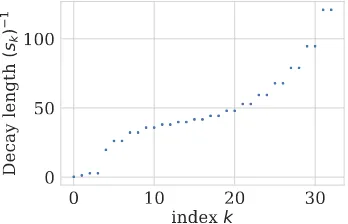
Figure 1.4: Decay lengths s−k1 for a power law 1/j1.5
H=H⊗L
j , and density operatorsρ in a Hilbert spaceH ⊗ H
∗ = [H
j⊗ H∗j]⊗L.
Closed-system Hamiltonian evolution, then, is d
dtρ=−i[H, ρ]≡ −iH
]ρ (1.129)
with a linear superoperator Hamiltonian defined H]:
H ⊗ H∗ → H ⊗ H∗,
H]=H⊗1−1⊗H. (1.130) For a spin-1/2 chain, we can writeSjx,y,z for operators on the ordinary (“ket”) spaceHj andTjx,y,zfor operators on the dual (“bra”) spaceH
∗
j; in this notation,
the superoperator corresonding to our fruit-fly Ising Hamiltonian (2.40) is H] =XHj]
≡X h(Sz jS
z
j+1−TjzT z j+1) +1
2h
x(Sx
j −T
x j ) +
1 2h
z(Sz
j −T
z j)
i
[image:38.612.220.394.240.352.2]WithH] in hand, we can proceed by Trotter decomposition, as with an MPS. 1.4.4 Matrix product density operator representations of Gibbs
states
1.4.4.1 Construction
In sections 2.3.3 and 2.3.4 we will require a Gibbs MPDO as our initial state. The Gibbs state is
ρ∝e−βH =e−βH/2Ie−βH/2 , (1.132) which is precisely the imaginary-time evolution of the product MPDO I by the Hamiltonian superoperator
Htherm] =H⊗1 + 1⊗H (1.133)
out to timeβ/2. We approximate this imaginary-time evolution not by tDMRG with the boustrophedon Trotter decomposition (1.114), but by ordinary TEBD using the trick of Hastings for numerical stability (as described in 7.3.2 of Schollw¨ock’s magisterial review [187], q.v.).
1.4.4.2 Estimating thermal expectation values
In analyzing the time evolution of ETH states, one naturally requires Gibbs state expectation values as a function of total energy (or, equivalently, energy density): the long time limit of an expectation value is given by its expectation value in a Gibbs state whose energy density matches that of the initial state. We tabulate energy densities and observables of interests for Gibbs states at a variety of temperatures using MPDOs as described above; to find the long-time limit of an expectation value, we measure the energy density of the initial state and linearly interpolate between the two nearest Gibbs energy densities. Note that this does not account for Trotter heating (that is, the fact that— because the system actually simulated is a Floquet system with period given by the Trotter step δt, its energy as measured by the Hamiltonian simpliciter gradually increases).
1.5 Some essentials of quantum thermodynamics
The classical Otto engine consists of a gas that expands, cools, contracts, and heats [179]. During the two isentropic (constant-entropy) strokes, the gas’s volume is tuned between values V1 and V2 < V1. The compression ratio is defined as r := V1
The engine outputs a net amount Wtot of work per cycle, absorbing heat Qin>0 during the heating isochore.
A general engine’s thermodynamic efficiency is
η:= Wtot Qin
. (1.134)
The Otto engine operates at the efficiency
ηOtto = 1− 1
rγ−1 < ηCarnot. (1.135) A ratio of the gas’s constant-pressure and constant-volume specific heats is denoted byγ := CP
Cv. The Carnot efficiencyηCarnot upper-bounds the efficiency
of every thermodynamic engine that involves just two heat baths.
A quantum Otto cycle for harmonic oscillators was discussed in Refs. [3, 51, 53, 102, 123, 190, 215, 244]. The quantum harmonic oscillator’s (QHO’s) gap plays the role of the classical Otto engine’s volume. Let ω and Ω > ω denote the values between which the angular frequency is tuned. The ideal QHO Otto cycle operates at the efficiency
ηQHO = 1− ω
Ω. (1.136)
This oscillator model resembles the qubit toy model that informs our MBL Otto cycle (Sec. 6.1).
The heat and work exchanged by slowly tuned systems are defined as
W :=
Z τ
0
dtTr
ρdH dt
and (1.137)
Q:=
Z τ
0
dtTr
dρ dt H
(1.138)
Thermalizing systems and
matrix product density
operators
C h a p t e r 2
SIMULATING QUANTUM DYNAMICS OF THERMALIZING
SYSTEMS
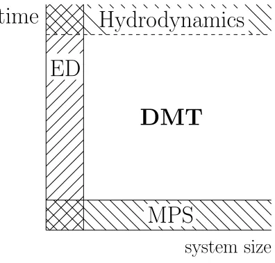
Questions about how (and whether) hydrodynamic behavior emerges from mi-croscopic quantum physics arise frequently in condensed matter physics. The exploration of this physics is hampered by the limitations of existing numerical methods (cf Fig. 2.1). Numerically exact methods (like exact diagonalization and Krylov subspace methods) can treat the dynamical properties of small systems at arbitrary times, but require memory and computation time expo-nential in system size. Matrix product state methods, on the other hand, can treat large systems—but only when the systems have little entanglement en-tropy. This means that for thermalizing systems, whose entanglement entropy grows linearly with time, MPS methods can only treat short-time behavior (see Figure 2.1).
This chapter describes a numerical method (“density matrix truncation” or “DMT”) based on matrix product representations of density operators. The
al-system size
time
MPS
ED
Hydrodynamics
[image:42.612.209.407.430.619.2]DMT
gorithm can accurately simulate not only short-time, low-entanglement behav-ior and long-time, hydrodynamic behavbehav-ior, but also the complex intermediate-time behavior from which the hydrodynamics emerges. While using matrix-product representations of mixed states is not new, the core of our algorithm is a new method for truncating matrix product density operators (MPDOs). This truncation exactly preserves the energy density of the system and other local conserved quantities, with the aim of leaving the hydrodynamics unaf-fected. It also avoids generating unphysical density matrices with negative entropy. At the same time, it is efficient enough that by taking large (but constant in system size) bond dimension one can capture the thermalization process.
We first (in Sec. 2.1) offer some background on matrix product state methods and intuition for why a method using MPDOs should be able to efficiently simulate time evolution governed by Hamiltonians satisfying the eigenstate thermalization hypothesis (ETH) to arbitrary times. We also motivate cer-tain properties of our method. We then describe (in Sec. 2.2) our algorithm for time evolution. This algorithm consists of the time-evolution framework described in Sec. 1.3 (cf [214]), paired with a novel scheme for truncating MP-DOs. We then apply our algorithm to time evolution starting from a pure state (Sec. 2.3.2) and find that it qualitatively improves upon existing meth-ods. Applied to a mixed state (Sec. 2.3.3 and Sec. 2.3.4), we find that our algorithm DMT matches or exceeds the state of the art. We conclude with directions we hope will improve on the method.
2.1 Background and intuition
2.1.1 Background: matrix product state methods
Simulating real-time evolution of many-body quantum-mechanical systems is hard: a system ofLsites generically requires storage and computation time ex-ponential inL. One line of attack, e.g. time-evolving block decimation (TEBD) [213, 214, 228], proceeds by representing unitary time evolution as a series of small time-steps applied to a matrix-product state (MPS) representation of a pure state. These matrix-product structures offer efficient representations of certain states (broadly speaking, “low-entanglement states”) in the sense that typical operations require polynomial time and memory.
product state, memory and computation time requirements grow exponentially in the entanglement entropy among the subsystems, so this linear growth in entanglement entropy sets a hard upper limit on the timescales on which ma-trix product states are useful, though a variety of methods have been used in attempts to circumvent this limit. [14, 58, 64, 78–81, 90, 157, 204, 223, 231]. One case in which entanglement growth does not limit the useful timescale of matrix product state simulations is the dynamics of many-body localized sys-tems, which exhibit a modest logarithmic entanglement growth [16, 192]. On the thermal side of the localization transition, however, entanglement grows quickly, and even the transition itself is expected to show extensive (volume-law) entanglement [76]—consequently, pure-state time evolution under Hamil-tonians remains restricted to short times.
Research into mixed-state time evolution and Lindblad dynamics has also pro-gressed. It has been proven that density matrices (and purifications) of Gibbs states of local Hamiltonians have efficient matrix product representations [85, 154, 163, 247]. Two schools of thought have used this insight to develop a series of methods for simulating time evolution. One school employs density matrices [21, 41, 95, 95, 101, 151, 152, 167, 168, 175–178, 212, 221, 222, 247]. They note that the space of operators on a spin chain is the tensor product of onsite operator spaces, just as the space of many-body pure states being a tensor product on onsite Hilbert spaces; the chief difference (in this view) is merely the dimensionality of the onsite space. For example, on a spin-half chain, the space of onsite operators is four-dimensional, while the space of pure states is two dimensional. This school then applies familiar pure state methods, including the creation and truncation of matrix product states and time evolution by TEBD, to density matrices—which are, after all, vectors in a larger space. The resulting truncation algorithms minimize the error ac-cording to the Hilbert-Schmidt (Frobenius) norm. In certain situations—in particular, dynamics near thermal equilibrium or a non-equilibrium steady state—this approach works well. In other situations, however—in particular, time evolution starting from a pure state—the density matrices suffer from a catastrophic loss of positivity. (Even checking positivity is NP-hard in the system size [117].)
so the system and ancillae together are in a pure state. Grouping each site and its ancilla into a larger onsite Hilbert space, one can write a matrix product representation for this pure state and apply the usual methods (truncation, TEBD, etc.) This solves the positivity problem: unlike density matrices, where many operators with reasonable matrix product representations are not posi-tive and hence are invalid as density matrices, every representable vector is a valid state. Moreover, since one can act with a unitary on the space of ancillae without changing the physical state, one can try to exploit this freedom to reduce the matrix product state bond dimension of the purification [17, 104]. There is also a hybrid approach which locally unzips a density matrix into a purification, which preserves positivity by construction [225]. These purifica-tion methods employ truncapurifica-tions which minimize error according to the inner product h·|·i defined on the whole (system with ancillae) state.
Neither the Frobenius norm on density matrices nor the quantum-mechanical norm on purifications is the correct notion of error. In the case of density matrices, the Frobenius norm fails to account for the fact that truncations that change the component of the density-matrix vector along the identity (i.e. which are not trace-preserving) are disastrous, because they can lead to loss of positivity. Moreover, neither notion of error captures spatial lo-cality: a good notion of error should prioritize short-range properties of the model and guarantee that certain quantities (the local conserved quantities of the model under consideration, like energy density or spin) are unchanged. Since the methods of both the density-matrix and purification schools generi-cally change the model’s conserved quantities at every gate application, they are unable in principle to approach the known “hydrodynamic” long-time be-havior of systems which thermalize. This may be the reason that existing density-matrix methods lose accuracy over time, even though one would ex-pect the accuracy of the matrix-product representation to improve as the state approaches equilibrium.
2.1.2 Intuition: thermalization and computation
Why should one be able to efficiently simulate the dynamics of a local Hamil-tonian satisfying the eigenstate thermalization hypothesis? In the long-time limit, the system is well described (as far as local observables are concerned) by a Gibbs state, which has an efficient matrix product density operator (MPDO) representation [85, 154]. Moreover, the system will (one expects) locally ther-malize before it reaches global equilibrium, and indeed after some short local thermalization time ttherm expectation values of local operators will be well approximated by the expectation values of those operators in a Gibbs state with spatially varying temperature, chemical potential, etc. Heuristically, one can imagine keeping the state exactly out to the local thermalization time and then truncating to an efficient representation. This would require a maximum bond dimension ca. (d2)vttherm, where v is some entanglement speed and d
is the dimension of the onsite Hilbert space. If vttherm is not too large, this approach itself may be workable.
In practice, however, one will wish to efficiently represent the state even at early and intermediate times t < ttherm—and also to avoid dependence on the hard-to-define and likely-unknown constant ttherm. Having decided upon an MPDO representation, then, one is faced with the problem of writing a truncation algorithm: an algorithm that will approximate a given MPDO by another, more compact MPDO.
The natural approach, by analogy with matrix product states, is to discard low-weight Schmidt vectors. (This approach turns out to be an imperfect solution, but it is a useful first step.) We call this truncation “Frobenius truncation.” A density operator is a vector in a space with the same tensor-product structure as a state, but a larger onsite dimension. We can therefore cut the chain at bond j into two sections L and R, Schmidt decompose, and truncate it:
ρ=
χ−1
X
α=0 ˆ
xLαsαxˆRα7→ χX0−1
α=0 ˆ
xLαsαxˆRα, χ0 < χ, (2.1)
where ˆxLα,xˆRαare operators supported onLandR, respectively, and trx
†
LαxLβ =
of the density operator
ρ=
χ−1
X
α=0
Aµ1
1 · · ·A
µj
j
αsα
Bµj+1 j+1 · · ·B
µL
L
ασˆ µ1
1 · · ·σˆ
µL
L (2.2)
whereAµl
l , B µl
l are χ×χ matrices—with the exception ofA µ1
1 andB
µL
L , which
are 1×χ and χ×1 respectively. We suppress for compactness a sum on µ (that is, on a basis for the space on onsite operators, here the Pauli matrices σµ with σ0 =I). The truncation (2.1) is then
ρ=
χ−1
X
α=0
· · ·Aµj
j
αsα
Bµj+1 j+1 · · ·
αˆσ
µ1
1 · · ·σˆ
µL
L
7→
χ0−1
X
α=0
· · ·Aµj
j
αsα
Bµj+1 j+1 · · ·
ασˆ
µ1
1 · · ·σˆ
µL
L ,
(2.3)
with χ0 < χ. This approximation minimizes the Frobenius (Hilbert-Schmidt)
norm distance—but a priori that is not the only norm one could use.
The Frobenius approximation scheme gives poor results for initial states far from equilibrium. One can see why by considering the expectation values of the operator Oylt = U(t)σlyU(t)† for a system that starts at t = 0 in a
product of σy eigenstates. (Note that Oy
l,t is a Schr¨odinger-picture operator
parametrized by time t. We work in the Schr¨odinger picture throughout, except where noted.) At timet,hψ(t)|Ol,ty |ψ(t)i=±1—but genericallyOyl,twill be a large, complicated operator (if