Recovering Structured Signals in High Dimensions via Non-Smooth Convex Optimization: Precise Performance Analysis

(1)

via non-smooth convex optimization:

Precise performance analysis

Thesis by

Christos Thrampoulidis

In Partial Fulfillment of the Requirements for the Degree of

Doctor of Philosophy

CALIFORNIA INSTITUTE OF TECHNOLOGY Pasadena, California

2016

(2)

c

2016

Christos Thrampoulidis ORCID: [0000-0001-9053-9365]

(3)

ACKNOWLEDGEMENTS

“As you set out for Ithaka hope the voyage is a long one, full of adventure, full of discovery. (...) Wise as you will have become, so full of experience,

you will have understood by then what these Ithakas mean."

Ithaka, C.P. Cavafy. Admittedly, the journey to this thesis has not been a paved way; it has gone through difficult and sometimes lonely paths, and it has been full of ups and downs. How-ever, during these five years I have been extremely lucky to have been surrounded by wonderful people -mentors, colleagues, friends, family- that have helped me the most in all aspects. It is thanks to them that “this voyage has been full of adventure, full of discovery and full of experience", and that I have grown both as a person and as a researcher. This is an opportunity to recognize my appreciation to them. First, I would like to express my gratitude to my advisor Prof. Babak Hassibi for his kindness, generosity, and patience; for the unstressful work environment and the academic freedom that he has provided me with, and for the guidance through-out this journey. His brightness, his enthusiasm, his clarity of thought, and his ability to communicate complex concepts -from a very diverse set of fields- in the most transparent ways have been an enormous inspiration. His provocative ques-tions and careful criticism have taught me to see the bigger picture, not only when presenting my work, but also as a guidance to new directions. His constant en-couragement has helped me grow confidence as a researcher. I am also grateful for several thought-provoking and always intriguing non-technical discussions, and for the opportunities he has provided me to travel and attend a number of conferences held all around the world.

(4)

pro-foundness, clarity and simplicity in teaching and in presenting his work.

I feel indebted to all my collaborators: Samet Oymak, Subhmonesh Bose, Ehsan Abbasi, Ashkan Panahi, Weiyu Xu, Linqi (Daniel) Guo, Kishore Jaganathan, and Navid Azizan, for their patience, for all the things that I learnt from them, and for all the fun and long hours that we spent thinking and learning together! Some of the major contributions and ideas of this thesis developed during long whiteboard discussions with Samet, Ehsan, and Ashkan. Thanks to Samet for introducing me to many of the problems addressed in this thesis. His unique combination of fast problem-solving skills, of hard work and of constant enthusiasm always inspired me. I also have some very good memories with Samet during our trip in Hawaii for ISIT. Thanks to Ehsan for all the technical work that we accomplished together. But even more so, I wish to thank him for his support and encouragement, for his endless patience, for being a great listener and a good friend. Thank you Ehsan, for the always pleasant and fun overnight shifts in the lab, for the handy Persian expressions that you taught me, for our amazing trip to Chicago, and for all the stories we shared together. Thanks to Ashkan and Daniel for our (rather) short but very productive collaboration. Thanks to Weiyu for helpful discussions and encouraging feedback. The works that we did together with Bose, Kishore, and Navid are not part of this thesis, but are by no means less important. Bose had the difficult task to be my first collaborator and coauthor. I am grateful to him for his patience, for teaching me the importance of communicating research results in a transparent way, and for his advice during the multiple times that I felt lost. Thanks toΚισώρος(cf., Kishore) for our joint work that led us win the Qualcomm Innovation Fellowship. I always admire his patience and calmness, and I confess that I sometimes laugh at his “jokes"! My collaboration with Navid has been only very recent, but one of the most pleasant ones, and I wish it continues.

(5)

and for being great listeners to my everyday complaints. I would especially like to express my gratitude to my good friend Wael, whom I have known since my very first days at Caltech.

Also, thank you to all other students in Caltech’s Electrical Engineering and Ap-plied Mathematics Departments for friendly interactions, advice and intriguing dis-cussions. Special thanks go to Roarke, Mark, Richard, and Yong Sheng. I would also like to thank the secretarial stafffor putting up with me and answering all my questions: Shirley, Tanya, Katie, Anne, Terecita, and Lucinda. My thanks also ex-tend to the friendly, welcoming, and always smiling administrative staffat Caltech’s International Student Programs Office and at Chandler Café.

Outside Caltech, I am grateful to Professors G. Moustakides, D. Toumpakaris, A. Birbas, A. Tzes, G. Bitsoris, T. Stouraitis, and S. Fassois from the University of Patras for their motivation and support when applying for graduate studies in the US. I am especially thankful to Prof. Moustakides for being a wonderful advisor during my undergraduate years, but also for the constant encouragement and guid-ance that I have been receiving from him since then. My gratitude extends to Prof. Toumpakaris for selflessly putting on long hours to help me complete my applica-tion files. I would also like to thank the “Andreas Mentzelopoulos Scholarships for the University of Patras" for supporting my studies during my first year at Caltech. A very special thank you belongs to my teacher Mr. Dimitris Aretakis and to my friend Stefanos Aretakis for teaching me and for making me love math.

(6)

Among the many wonderful people that I have met during this journey, I would like to especially acknowledge Panagiotis Vergados, Juan Andrés Muniz, Wael Hal-bawi and Georgia Papadakis, who have been great friends and have kept me sane and happy over the years. Thank you for your honesty, for your kindness, and for caring for me not only when the sun is shining, but most importantly during the storms. (Yes, there were storms despite the California weather!) Thank you for all the memories that we have shared; thank you for every single day. Panagiotis, ad-ditional thanks go to you for the long hours that you selflessly put on proofreading parts of this thesis and providing invaluable feedback on my thesis presentation! I am also thankful to my extended family in Veroia, Ptolemaida, Thessaloniki and Patras for always being there for me, for their love, and for their heartfelt support during all these years. Thank you for always cutting a cake for my birthday even if I had to blow out the candles and eat my piece of it over Skype!

(7)

To my parents Vassiliki and Kleanthis,

and to my brother Manolis.

Στους γονείς μου Βασιλική και Κλεάνθη,

(8)

ABSTRACT

The typical scenario that arises in modern large-scale inference problems is one where the ambient dimension of the unknown signal is very large (e.g., high-res-olution images, recommendation systems), yet its desired properties lie in some low-dimensional structure such as, sparsity or low-rankness. In the past couple of decades, non-smooth convex optimizationmethods have emerged as a powerful tool to extract those structures, since they are often computationally efficient, and also they offer enough flexibility while simultaneously being amenable to perfor-mance analysis. Especially, since the advent of Compressed Sensing (CS) there has been significant progress towards this direction. One of the key ideas is that random linear measurements offer an efficient way to acquire structured signals. When the measurement matrix has entries iid from a wide class of distributions (including Gaussians), a series of recent papers have established a complete and transparent theory thatpreciselycaptures the performance in the noiselesssetting. In the more practical scenario ofnoisymeasurements the performance analysis task becomes significantly more challenging and correspondingpreciseandunifying re-sults have hitherto remained scarce. The available class of optimization methods, often referred to asregularized M-estimators, is now richer; additional factors (e.g., the noise distribution, the loss function, and the regularizer parameter) and sev-eral different measures of performance (e.g., squared-error, probability of support recovery) need to be taken into account.

This thesis develops a novel analytical framework that overcomes these challenges, and establishes precise asymptotic performance guarantees for regularized M-esti-mators under Gaussian measurement matrices. In particular, the framework al-lows for a unifying analysis among different instances (such as the Generalized LASSO, and the LAD, to name a few) and accounts for a wide class of perfor-mance measures. Among others, we show results on the mean-squared-error of the Generalized-LASSO method and make insightful connections to the classical the-ory of ordinary least squares and to noiseless CS. Empirical evidence is presented that suggests the Gaussian assumption is not necessary. Beyond iid measurement matrices, motivated by practical considerations, we study certain classes of ran-dom matrices with orthogonal rows and establish their superior performance when compared to Gaussians.

(9)

rate (BER) of the popularconvex-relaxation of the Maximum Likelihood decoder for recovering BPSK signals in a massive Multiple Input Multiple Output setting. Our precise BER analysis allows comparison of these schemes to the unattainable Matched-filter bound, and further suggests means to provably boost their perfor-mance.

The last challenge is to evaluate the performance undernon-linearmeasurements. For the Generalized LASSO, it is shown that this is (asymptotically) equivalent to the one under noisy linear measurements with appropriately scaled variance. This encompasses state-of-the art theoretical results of one-bit CS, and is also used to prove that the optimal quantizer of the measurements that minimizes the estimation error of the Generalized LASSO is the celebrated Lloyd-Max quantizer.

(10)

7.6 `2-LASSO . . . 105

7.7 `2₂-LASSO . . . 109

7.8 The NSE of Generalized LASSO with Arbitrary Fixed Noise . . . . 114

7.9 The Worst-Case NSE of Generalized LASSO . . . 121

Chapter VIII: Beyond iid Ensembles: Isotropically Random Orthogonal Ma-trices . . . 123

8.2 Results . . . 126

8.3 Proof Outline . . . 130

Chapter IX: Beyond Squared-error: General Performance Metrics . . . 133

9.2 Review: `2-reconstruction Error . . . 135

9.3 Lipschitz Performance Metrics . . . 136

9.4 Support Recovery . . . 138

9.5 Proofs . . . 140

Chapter X: Application: The Bit-Error Rate of the Box-Relaxation Optimiza-tion . . . 143

10.1 BPSK Signal Recovery . . . 144

10.2 Implications . . . 145

10.3 Extensions . . . 148

Chapter XI: Non-linear Measurements . . . 151

11.1 Motivation & Contribution . . . 152

11.2 Results . . . 157

11.3 Application: Optimalq-bit Quantization . . . 160

Chapter XII: Conclusions and Future work . . . 164

Appendix A: Proofs for Chapter 3 . . . 184

Appendix B: Proofs for Chapter 4 . . . 189

Appendix C: Proofs for Chapter 6 . . . 227

Appendix D: Calculating the Summary Parameters . . . 236

Appendix E: Proofs for Chapter 8 . . . 240

Appendix F: Proofs for Chapter 10 . . . 250

Appendix G: Proofs for Chapter 11 . . . 255

(12)

LIST OF FIGURES

Number Page

2.1 Illustration of the Null-space condition (Proposition 2.2.1). . . 11 2.2 Illustration of the distance of a vector to the scaled subdifferential

λ∂f(x0) and to the cone of subdifferential cone(∂f(x0)). . . 16

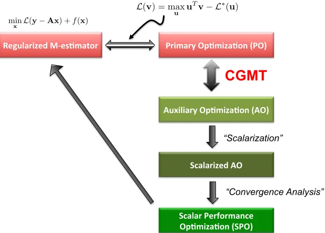
5.1 Schematic representation of the CGMT framework. The first step

in-volves equivalently expressing the regularized M-estimator as a

min-max Primary Optimization (PO) (cf. (3.11a)). (These problems are

hard to directly analyze and are thus shown in red.) The CGMT

Theorem 3.3.1 associates with the (PO) an Auxiliary Optimization

(AO) problem that is simpler to analyze (hence, depicted in green). The second step of the framework involves simplifying the (AO) into

an optimization problem that only involves scalar variables. This

makes possible the convergence analysis that follows as a third step

and leads to a deterministic Scalar Performance Optimization (SPO).

The last step involves using the (SPO) to conclude about the original

regularized M-estimator. . . 61 6.1 Using the predictions of Theorem 4.2.1 to analytically compare the

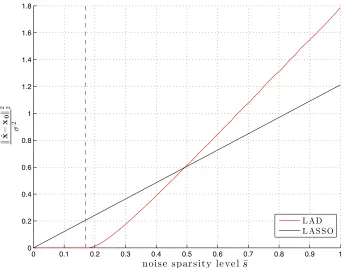
performance of different instances of M-estimators. Here, we

com-pare a least-absolute deviations (LAD) to a least-squares (LASSO) loss function in (6.16) for sparse signal estimation under sparse noise.

The normalized squared error is plotted as a function of the

sparsity-level ¯sof the noise at the high-SNR regime. The noise is sparse with

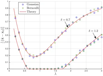
sparsity level ¯s and nonzero entries are i.i.dN(0, σ2) andσ2 → 0. Also, the sparsity level of the unknown signal is fixed to be 0.1 and the normalized number of measurements isδ =3/5. . . 77 6.2 Squared error of thel1-Regularized LAD with Gaussian (◦) and Bernoulli

() measurements as a function of the regularizer parameter λ for two different values of the normalized number of measurements, namely δ = 0.7 and δ = 1.2. Also, x0,i iid∼ px(x) = 0.9δ0(x) +

0.1φ(x)/√0.1 and zj iid∼ pz(z) = 0.7δ0(z) + 0.3φ(z) for φ(x) = 1

√

2πe−x

2_/2

. For the simulations, we used n = 768 and the data were

(13)

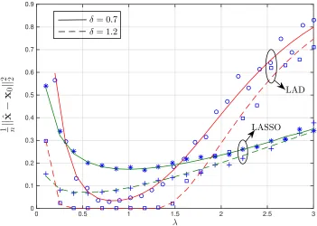
6.3 Comparing the squared error of the `1-Regularized LAD with the

corresponding error of the LASSO. Both are plotted as functions of

the regularizer parameter λ, for two different values of the

normal-ized measurements, namely δ = 0.7 and δ = 1.2. The noise and signal are iid sparse-Gaussian as follows: x0,i iid∼ px(x)=0.9δ0(x)+

0.1φ(x)/√0.1 and zj ∼ pz(z) = 0.9δ0(z) + 0.1φ(z) with φ(x) = 1

√

2πe−x

2_/2

. For the simulations, we used n = 768 and the data were

averaged over five independent realizations. . . 86 6.4 Squared error of the `1-Regularized M-Estimator with Huber-loss

as a function of the regularizer parameter λ. Here, δ = 0.7, x0 iid

∼ px(x)=0.9δ0(x)+0.1φ(x)/

√

0.1 andpz(z)= 0.9δ(z)+0.1η(z) with φ(x) = _√1

2πe

−x2_/2

andη(z) = _π(11₊_z2₎. For the simulations, we used

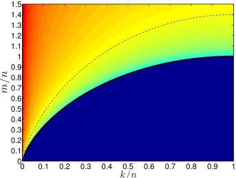
n=1024 and the data are averaged over 5 independent realizations. . 87 7.1 NSE heatmap for `1 minimization based on Theorem 7.5.1. The

x and y axes are the sparsity and measurements normalized by the

ambient dimension. To obtain the figure, we plotted the heatmap of

the function −log D(cone(∂f(x0)))

m−D(cone(∂f(x0))) (clipped to ensure the values are

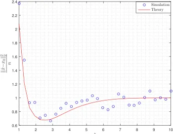
between [−10,5]). . . 104 7.2 Regions of operation of the`2-LASSO. . . 107 7.3 We consider the`1-penalized`2-LASSO problem for ak sparse

sig-nal in Rn. For k_n = 0.1 and m_n = 0.5, we haveλcrit ≈ 0.76, λbest ≈

1.14, λmax≈1.97. . . 108

7.4 Illustration of the regionR_ON and of the map function (Defn. 7.7.2) for f = k · k₁andx0 ∈ Rn ak-sparse vector. map−1maps the value

of the regularizerλin (7.3) to a value in R_ON. Df,x0(τ) andCf,x0(τ)

are computed as in (7.40). . . 112 7.5 Numerical validation of Theorem 7.7.1 for f = k · k₁ and x0 ∈ Rn

ak-sparse vector. Measured values of the NSE(σ) are averages over

50 realizations ofA,v. The theorem accurately predicts NSE(σ) as

(14)

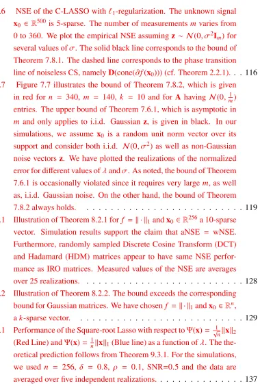
7.6 NSE of the C-LASSO with`1-regularization. The unknown signal

x0 ∈ R500is 5-sparse. The number of measurements m varies from

0 to 360. We plot the empirical NSE assuming z ∼ N(0, σ2Im) for several values ofσ. The solid black line corresponds to the bound of Theorem 7.8.1. The dashed line corresponds to the phase transition

line of noiseless CS, namelyD(cone(∂f(x0))) (cf. Theorem 2.2.1). . . 116

7.7 Figure 7.7 illustrates the bound of Theorem 7.8.2, which is given

in red for n = 340, m = 140, k = 10 and for A having N(0, _m1) entries. The upper bound of Theorem 7.6.1, which is asymptotic in

m and only applies to i.i.d. Gaussian z, is given in black. In our

simulations, we assume x0 is a random unit norm vector over its

support and consider both i.i.d. N(0, σ2) as well as non-Gaussian noise vectors z. We have plotted the realizations of the normalized error for different values ofλandσ. As noted, the bound of Theorem

7.6.1 is occasionally violated since it requires very large m, as well

as, i.i.d. Gaussian noise. On the other hand, the bound of Theorem

7.8.2 always holds. . . 119 8.1 Illustration of Theorem 8.2.1 for f = k · k₁andx0 ∈R256a 10-sparse

vector. Simulation results support the claim that aNSE = wNSE.

Furthermore, randomly sampled Discrete Cosine Transform (DCT)

and Hadamard (HDM) matrices appear to have same NSE

perfor-mance as IRO matrices. Measured values of the NSE are averages over 25 realizations. . . 128 8.2 Illustration of Theorem 8.2.2. The bound exceeds the corresponding

bound for Gaussian matrices. We have chosenf = k · k₁andx0 ∈Rn,

ak-sparse vector. . . 129 9.1 Performance of the Square-root Lasso with respect toΨ(x)= √1

nkxk2 (Red Line) andΨ(x)= 1_nkxk₁(Blue line) as a function ofλ. The the-oretical prediction follows from Theorem 9.3.1. For the simulations,

we used n = 256, δ = 0.8, ρ = 0.1, SNR=0.5 and the data are

[image:14.612.128.508.64.628.2]

(15)

9.2 Probability of successful recovery of the on-support and of the off

-support entries as a function ofλfor two different values of the

nor-malized measurements, namelyδ = 0.8 (solid) andδ =1.2 (dashed).

The theoretical prediction (shown in solid/dashed lines) follows from Theorem 9.4.1. For the simulation points (shown with squares and

circles), we used n = 256, SNR= 0.5, = 10−3, ρ = 0.1 and the data are averaged over five independent realizations of the problem. . 139 10.1 Bit error rate performance of the Boxed Relaxation: BE R as a

func-tion of SNR for different values of the ratioδ = dm/ne of receive to transmit antennas. The theoretical prediction follows from Theorem

10.1.1. For the simulations, we used n = 512. The data are

aver-ages over 20 independent realizations of the channel matrix and of

the noise vector for each value of the SNR. . . 146 10.2 Bit error rate of the Box Relaxation Optimization (BRO) in (10.1) in

comparison to the Matched Filter Bound (MFB) forδ =0.7 (dashed

lines) andδ = 1 (solid lines). The red curves follow the formula of

Thm. 10.1.1, the green ones correspond to (10.4), and, BERM F B of

(10.5) is in blue. . . 148 10.3 Bit error rate of the Box Relaxation Optimization (BRO) in (10.6) as

a function of the SNR for BPSK, 4-PAM and 8-PAM signals. The

theoretical prediction follows from Theorem 10.3.1. For the

simu-lations, we used n = 512 andδ = 1.2. The data are averages over 20 independent realizations of the channel matrix and of the noise

vector for each value of the SNR. . . 149 11.1 Squared error of the`1-regularized LASSO with non-linear

measure-ments () and with corresponding linear ones (?) as a function of the regularizer parameterλ; both compared to the asymptotic prediction.

Here, gi(x) = sign(x +0.3zi) with zi ∼ N(0,1). The unknown sig-nal x0 is of dimension n = 768 and has d0.15ne non-zero entries.

(16)

11.2 Squared error of the`1-regularized LASSO as a function of the

reg-ularizer parameter for noisy 1-bit measurements gi(x) = sign(x + 0.3zi). Here,x0is sparse with pX0(+1) = pX0(0)= 0.05, pX0(+1) =

0.9. The theoretical prediction is obtained by Corollary 11.2.1. Fi-nally, δ = 0.75, n = 512, and the simulation points represent

aver-ages over 20 realizations. . . 160 11.3 Squared error of the group-sparse LASSO as a function of the

reg-ularizer parameter compared to the asymptotic predictions for noisy

1-bit measurementsgi(x)=sign(x+0.3zi). Here,x0is group-sparse:

it is composed oft =512 blocks of block sizeb =3, and each block is zero with probability 0.95, otherwise its entries are iid N(0,1). The theoretical prediction is obtained by Corollary 11.2.1. Finally, δ = 0.75, and the simulation points represent averages over 20 real-izations. . . 161 11.4 Illustration of the equivalence result of Theorem 11.2.1 applied to

quantized measurements. . . 162 B.1 Graphs of the Moreau envelope functions of a quadratic (left) and

of the absolute value (right), for different values of the parameterτ.

Moreau envelopes are alwayssmooth under-estimators of the

(17)

LIST OF TABLES

Number Page

(18)

C h a p t e r 1

INTRODUCTION

“Big data" and accompanying terms such as “data-analytics" and “data-science" have grown to become some of the hottest and most overused buzzwords over the past few years [Mac16;Pel15;Flo16]. This terminology has, by now, proliferated across the world of academia and has invaded a lot of academic conversations, pre-sentations, and research agendas. Certainly, there is a lot of hype over big data, but no one can argue against the following fact: today’s world is awash with data originating from numerous different disciplines (e.g. image processing, wireless communications, sensor networks, machine learning, financial data, genomics sig-nal processing, and DNA microarrays) that are gathered by all means at an increas-ingly fast pace, and major efforts are underway to extract valuable information from them. A common theme among such instances of massive automatic data collec-tion isdata outputs, which are comprised of many observations/measurements, but even more so, of a larger and larger number of variables of interest. This is very different from the traditional assumption behind classical tools in estimation theory, under which only a few well-chosen variables are of interest.

To make ideas concrete, consider the fundamental statistical inference task of re-covering an unknown signal from noisy linear measurements:

y=Ax0+z, (1.1)

Henceforth,ydenotes the vector of (say)mmeasurements,x0is the unknown signal comprised of n variables, A is the measurement matrix and z is the noise vector. In the “classical world", the pervasive modeling assumption is that the number of variables n is fixed and small while m grows large. Here, there is a complete set of tools that can derive good estimates ˆxofx0. Importantly, an intellectually clean theoretical framework accompanies this set of tools withperformance guarantees under all sorts of different settings (e.g., in the presence of outliers, deviations in the model, and so on). Unfortunately, the classical tools and theory are mostly inadequate to cope with the dimensionality explosion that we experience in today’s applications.

(19)

a large-scale image produced from magnetic resonance imaging (MRI), the human genome, or a vector of transmitted symbols in a massive MIMO scenario). More-over, it is common that the number of measurements m is less than the number of variables n. For example, there are many genes, but only few patients with a given genetic disease, and, in applications like MRI there is not enough time to collect many observations [Don+00]. On the face of it, this makes the problem ill-posed (as the system of Equation in (1.1) becomes underdetermined). Fortunately, the signal of interest is often constrained structurally so that it only has a few de-grees of freedom relative to its ambient dimension. For instance, MRI images often admit sparse representations in appropriate transform domains [CRT06], transmit-ted symbols belonging to finite constellations (e.g. m-PAM, m-QAM) only take values belonging to a finite alphabet, and covariance matrices are often well ap-proximated by low-rank matrices. In summary, modern inference procedures and accompanying theory are developed in view of the following distinguishing features ofhigh-dimensional inferenceproblems:

(i) large number of variables to be estimated (largen), (ii) (often) compressed measurements (m < n),

(iii) signals typically possess low dimensionalstructure(e.g., sparsity, low-rankness).

In this context, a new set of high-dimensional signal processing and statistics tools is required, ones that have the following favorable properties: the ability to reveal those structures and operate under a compressed number of measurements; compu-tational efficiency; robustness to outliers, to model misspecification, and to miss-ing data; and also, optimality guarantees. Among different approaches, convex-optimization based ones are often preferred since they offer enough flexibility and at the same time are usually amenable to analysis, simultaneously, with regard to computation, asymptotic theory and intuitive interpretation.

Over the past couple of decades,non-smooth convex optimization has emerged as a powerful structure-extracting tool for high-dimensional inference. These proce-dures obtain estimates ˆxof the unknown signalx0 by solving convex programs of the form:

ˆ

x=arg min

(20)

Henceforth, L represents a convex loss function that penalizes the residual, f is a convex (typically non-smooth) regularizer, and, λ > 0 is a regularizer parameter. Often, such estimators are referred to asregularized M-estimators, which includes for example,`1-penalized least-squares (aka LASSO), penalized least-absolute de-viations (aka LAD), and, regularized Maximum-likelihood estimators. Regularized M-estimators have been around for at least twenty-years and have enjoyed great success in practice. In fact, the non-regularized versions (i.e., f = 0) of (1.2) correspond to the “plain vanilla" regression M-estimators, which were proposed and have been analyzed under the classical statistical setting since at least the 70s [Hub11]. The idea of adding a non-smooth regularizer to exploit the underlying structure of the unknown signal is also relatively old [CM73;SS86], but it appears to have gained significant popularity and attention starting in the mid 90’s [Tib96;

CDS98] and even more so about a decade ago in the context ofCompressed Sensing [CRT06;Don06a].

The convex nature of (1.2) can in principle lead to corresponding tractable numer-ical algorithms. In particular, many of these programs (e.g. `1 and nuclear-norm penalized least-squares) are instances of convex conic programs, and so they can be solved in polynomial time using (say) interior point methods [BV09]. However, such standard solvers for convex programming, are often prohibitively computa-tionally intense for modern large-scale data sets. This has led to an increasing interest in deriving and analyzing the convergence properties of simpler first-order methods (e.g., projected gradient-descent) that aim to make (1.2) scalable in high-dimensions (e.g., see [TA16;ZL15;ORS15;Bru+14] and references therein). Re-lated algorithmic efforts involve designing solvers that can solve (1.2) in a dis-tributed manner among different machines (e.g., [Rec+11]).

Rather than algorithmic issues, this thesis studies the fundamentalanalytical ques-tions related to the inference performance of (1.2):

How good an estimator of the true unknown signalx0

(21)

cross-validation. The idea here is to split the data set (in our context, the pairs (y,A)) into a training set and a validation set: an estimate ˆxis obtained by solving (1.2) based on the training set and its quality is evaluated on the rest of the data. In this thesis we follow an analytical approach: we assume that the measure-ment matrix A is realized from the ensemble of m × n matrices with entries iid standard normal and derive anexact asymptotic characterization of the estimation quality of regularized M-estimators. The assumption on the random nature of the measurement matrix is by now a benchmark in the field of Compressed Sensing and high-dimensional signal-processing1: randomly generated matrices can prov-ablyyield good estimates of ˆx0from compressed high-dimensional measurements [FR13;EK12;Boc+15]. Matrices sampled from the Gaussian ensemble have been traditionally useful in analytical works in random matrix theory and Compressed Sensing has been no exception to that rule2. In fact, one of the finest and most el-egant (analytical) successes of the field corresponds to an exact characterization of the absolute minimum number of measurements required as a function of the struc-tural complexity of the unknown signal, in order for convex optimization algorithms of the form in (1.2) to perfectly recover the signal in theabsence of noise. These are known asphase-transitionresults in the literature of noiseless Compressed Sensing (see Section2.2for a survey of references).

One of the main contributions of this thesis is an extension of these results to the noisy case. When compared to the noiseless setting, the analysis under the presence of noise is not only more practical but is also inherently more challenging since: (a) one has to predict the precise value of the estimation error, rather than just discriminating between perfect recovery or not; (b) the performance depends not only on the number of measurements but also on the noise and signal statistics; (c) the optimization itself involves additional parameters that contribute to the final prediction.

Extensions of the theory to matrices (a) with entries drawn iid from other measure-ment ensembles, (b) with random orthogonal rows, and (c) ones that are elliptically

1_{For example random matrices have been known to be useful for dimensionality-reduction}

pur-poses since at least the mid 80’s [JL84]

2_{Admittedly, this is a very special case of possible distributions of}_A_{; in a large extent this is}

(22)

distributed are also discussed. For instance, we derive explicit formulae charac-terizing the estimation performance under a certain class of orthogonal matrices (the isotropically random ones), and establish their superior performance when compared to Gaussians. Notably, we empirically observe that the same formulae continue to hold true for random Discrete Cosine Transform (DCT) and Hadamard matrices, which are often preferred in practice since they allow for fast multiplica-tion and reduced storage complexity.

An important feature of the exact nature of the estimation predictions derived in this thesis is that they can be used to compare performance between different in-stances of regularized M-estimators. This lays the groundwork towardsdeveloping a complete theory of regularized M-estimators in the high-dimensional regimethat involves providing rigorous answers to optimality questions regarding the choice of the involved parameters:

– What is the optimal loss function and regularizer, under different settings, e.g., in the presence of outliers, particular structure ofx0?

– What is the minimum achievable squared error in each one of those scenar-ios? Under what conditions canx0be recovered with zero error?

– How may the regularizer parameterλbe optimally tuned? – How does the sampling ratioδ = m/naffect the error?

– How robust is the estimation to deviations from the linear model in(1.1)?

In the course of this thesis, we provide answers to some of the questions above3. For instance, we answer the last question by evaluating the performance of (say) reg-ularized least-squares (aka Generalized LASSO) under measurements of the form

y = g(Ax0), where g is a possibly unknown, random and nonlinear link function that aims to capture potential model miss-spesifications in (1.1).

Nonlinear measurements of this form might also arise by design (e.g. quantized measurements), in which case, our theoretical results lead to new opportunities in theoptimal designof the nonlinear link function (e.g. by choice of the thresholds

3_{It is worth repeating that the high-dimensional regime of interest di}_ff_{ers from the classical}

(23)

and levels of quantization). For an illustration, we prove that the optimal quantizer of the measurements that minimizes the estimation error of the Generalized LASSO is the celebrated Lloyd-Max quantizer.

(24)

C h a p t e r 2

BACKGROUND, LITERATURE SURVEY AND SUMMARY OF

CONTRIBUTIONS

The chapter begins with a survey on the theory of phase-transitions of convex op-timization innoiselesslinear inverse problems, which has been developed in a se-ries of recent papers [DT09a;Sto09b;Cha+12;BLM+15;Ame+13; Sto13b], and which is an essential precursor to the material of this thesis. The rest of the chapter discusses in detail the scope and contributions of this dissertation.

Section2.1 introduces some key ideas that have emerged from the existing theory of Compressed Sensing (CS). Section2.2reviews the theory of phase transitions in noiseless CS in some detail and surveys the relevant literature. In Section2.3 we see that the presence of noise imposes additional challenges in the analysis. This leads us to Section2.4, where we set the main objectives of this thesis and survey its contributions on a chapter by chapter basis.

2.1 Compressed Sensing

(25)

that were developed during these years are as follows:

(i) Exploit the underlying low-dimensional structure of the unknown signal. Spar-sity is only one such example of structure. Other often encountered examples include signals that are block-sparse, low-rank, slow-varying, take values over a finite alphabet, and so on. It has been recently recognized that recovery and analysis techniques that were initially developed for the problem of sig-nal recovery extend naturally to other kinds of structures [Cha+12;Ame+13;

FM14;OTH13b; TAH16]. Of course, such aunifyingviewpoint has, among others, the clear advantage of enlarging the scope and applicability of the de-veloped theory.

(ii) Use of random measurement matrices. The value of randomness in the mea-surement matrix model was recognized in the early work of Candes, Romberg and Tao [CT06] and has remained crucial in most subsequent literature. Ran-domness can be expressed in various forms (e.g. entrees sampled iid from various distributions, randomly subsampled Fourier matrices, etc.) and of-ten guarantees the required incoherence property between the sampling ma-trix and the unknown vector, which makes the recovery problem well-posed. Moreover, the randomness turns out to be crucial in establishing analytical results. From a practical perspective, the randomness assumption is most rel-evant in applications where one has the freedom of designing the measurement matrix. Yet, valuable intuitions can be gained in instances where this is not the case.

(iii) Use of recovery methods that are based on convex programming techniques. This idea can be traced back very early in the literature [CM73;SS86]. In the context of sparse approximation the idea that gives rise to BP is to replace the original`0-minimization formulation of the problem by its convex relax-ation, the `1-minimization. Of course, the same idea goes beyond sparsity and extends to more general notions of structure. As already mentioned, the advantage of convex methods is that they often lead to tractable numerical algorithms as well as to insightful statistical performance analyses.

(26)

Linear Inverse Problems and Convex Optimization

The classical setting of CS is that of linear inverse problems, which assume noisy linear measurements y = Ax0 + z ∈ Rm of an unknown, but structured, signal x0 ∈ Rn. To keep things general, we do not specify the particular structure of x0, although is assumed known to us; it could be sparsity, group-sparsity, low-rankness, and so on. We are particularly interested in the scenario of compressed measurements, i.e. m < n, and the goal is that of estimatingx0.

Towards this goal, non-smooth convex optimizationtechniques have emerged as a powerful technique. As already mentioned in Chapter1, these methods produce an estimate ˆxofx0by solving (1.2). The loss functionL aims to fit the final estimate to the observations based on the linear measurement model. On the other hand, the regularizer function f aims to exploit the particular structure of the unknown signal x0. For instance, it is by now well-understood in the CS literature that `1 -regularization promotes sparsity,`1,2-regularization is appropriate for group spar-sity, and nuclear-norm-regularization promotes low-rank solutions. In fact, there are principled ways to construct such convex regularizer functions based on the idea of representing the low-dimensional structure ofx0as a decomposition into afew well-selectedatoms[Cha+12]. The atomic-decomposition framework has roots in non-linear approximation [Jon92;Bar93] and was formally introduced in the context of noisy linear inverse problems under compressed measurements by Chandrasekaran et. al. in [Cha+12]. The framework explains in a principled and insightful way why

`1-minimization and nuclear-norm are natural candidates for sparse and low-rank recovery, respectively, and generalizes the construction to several other types of low dimensional structures [Cha+12]. It should be mentioned that other recipes for associating convex regularizers to corresponding low-dimensional structures have been considered in the literature (e.g., [Bac10;BCW10]). A detailed review of all these goes beyond the scope of this thesis.

For the purposes of our discussion it is important to note that f in (1.2) aims to pro-mote the structure ofx0and that typically good choices correspond to non-smooth functions (e.g. `1-norm, nuclear-norm). The fact that f is typically non-smooth imposes additionally challenges in the assessment of the estimation performance of (1.2), since the solution ˆx does not admit a closed-form expression (for example, this would be the situation in the case of a quadratic L function with a quadratic regularization, also known as ridge-regression).

(27)

Question (Q.1). We start by discussing the noiseless case (i.e. z=0in (1.1) in Sec-tion 2.2, where recent studies provide an exact answer through a mathematically clean, elegant and general theory. Answering Question (Q.1) in the presence of noise is more challenging, and this is what this thesis focuses on addressing. Cor-responding exact results in the literature are scarce and limited to specific instances of (1.2).

2.2 Noiseless Case

In the absence of noise, the measurements satisfy y = Ax0. Naturally then (1.2) reduces to the following constrained convex minimization problem1:

ˆ

x= arg min

y=Axf(x). (2.1)

Since measurements are noiseless, we hope that the unknown signalx0 can be re-covered exactly, i.e. ˆx = x0. Consequently, the fundamental question (Q.1) essen-tially reduces to the following:

Under what conditions is the solutionxˆ of (2.1) unique and equal tox0? (Q.2)

Null-space Condition

When ˆx = x0 is the unique solution of (2.1), we say that the program succeeds, otherwise it fails. A necessary and sufficient condition for success of (2.1) is known as the “null-space condition" and is given in the lemma below. LetN(A) denote the null-space of the measurement matrixAandT_f(x0) the tangent cone of f atx0, as defined below:

Definition 2.2.1(Tangent Cone). The tangent cone T_f(x0) of f atx0 is defined as the closure of the conic hull of the set of descent directionsD_f(x0) of f atx0:

D_f(x0) :={v| f(x0+v) ≤ f(x0)}.

Proposition 2.2.1 (Null-space Condition). x0 is the unique minimizer of (2.1)iff

N(A)∩ D_f(x0) = {0}, or equivalently,

N(A)∩ T_f(x0)= {0}. (2.2) The proof of the proposition is almost straightforward but is included for com-pleteness. See Figure 5.1 for a simple schematic representation of the null-space condition for the case of sparse recovery using`1-minimization.

1_{Besides convex relaxation based schemes, other signal recovery methods such as greedy}

(28)

[image:28.612.136.475.72.262.2]

Figure 2.1: Illustration of the Null-space condition (Proposition2.2.1).

Proof. (of Proposition 2.2.1). It is convenient to change the variable in the opti-mization in (2.1) to theerror vector w=x−x0. This gives

min

Aw=0f(x0+w). (2.3)

We show that ˆw=0 is the unique solution to this minimization iffN(A)∩ T_f(x0) =

{0}. Letv ∈ N(A)∩ D_f(x0). Clearly,Av = 0 andvis feasible in (2.3). Moreover, f(x0 + v) ≤ f(x0) by definition of the set of descent directions. Combined, v is a minimizer of (2.3), which completes the proof. The equivalence of the two conditions in the statement of the proposition follows by Definition 2.2.1and the

fact thatN(A) is a linear subspace.

Condition2.2.1is geometric in nature: “When does the null-space of the measure-ment matrix not intersect (other than at0, of course) the tangent cone?". Checking this for deterministic matrices is hard. However, it turns out to be tractable when

Apossesses specific randomness properties. WhenAis realized from some proba-bility ensemble, then it is desirable to satisfy Condition (2.2)with high probability (whp) over the matrix realization.

Gaussian Matrices: Escape through a mesh&Gaussian width

(29)

answer to this question was given by Gordon in 1988 [Gor88] and is known as the “escape through a mesh lemma". Gordon proved and used the lemma in a different context; Rudelson and Vershynin first noticed its relevance to the CS problem in 2006 [RV06], in the context of sparse signal recovery.

Before stating the lemma, we will introduce two very useful concepts, namely the “minimum conic singular value" (mCSV) and the “conic Gaussian width".

Definition 2.2.2 (Minimum conic singular value). LetA ∈ _Rm×n. The minimum conic singular value ofAwith respect to a coneK ⊂ _Rnis defined as,

σmin(A;K)= inf

w∈K ∩Sn−1kAwk2.

Henceforth,Sn−1denotes the unit sphere inRn. To see the relevance of Definition 2.2.2to our discussion, observe that

σmin(A;T_f(x0))> 0 ⇒ (2.2) holds. (2.4) Also, note thatσmin(A;Rn) is the minimum singular value ofA.

Definition 2.2.3(conic Gaussian width). Leth ∈_Rn have entries iid standard nor-mal. The Gaussian width of a cone (not necessarily convex)K ⊂ _Rnis denoted by

ω(K) and is defined as:

ω(K) :=_E

sup

w∈K ∩Sn−1

hTw,

where the expectation is over the randomness ofh.

The Gaussian width is a geometric measure of the size of the cone and plays a central role in asymptotic convex geometry [AAGM15;LT91].

Proposition 2.2.2(Escape through a mesh). LetA ∈ _Rm×n have entries iid stan-dard normal andK be a cone inRn. Then, for anyt > 0, it holds with probability at least1−e−t2/2that

σmin(A;K) ≥

√

m−1−ω(K)−t.

(30)

Combining Proposition2.2.2with (2.4) and Proposition2.2.1, shows that, when the measurement matrix is Gaussian, the convex program (2.1) succeeds with exponen-tially high probability, as long as the number of measurements satisfies

m ≥ (ω(T_f(x0))−t)2+1. (2.5) In this sufficient condition for successful recovery, the role of the regularizer func-tion f and the particular structure ofx0 are summarized by the Gaussian width of the tangent cone ω(T_f(x0)). Certainly, (2.5) is alone a remarkable result. Yet, it would be of limited practical use unlessω(T_f(x0)) can be computed for interesting regularizers and for corresponding structures. Thankfully, it will be soon shown that this indeed the case! Towards this direction, note from (2.5) that any upper bound on the Gaussian width translates to a sufficient lower bound on the required number of measurements for successful recovery. Importantly, it turns out that for many examples of structured signals that are encountered in practice, there exist good choices of the regularizer function such that

ω2₍_T

f(x0)) n. (2.6)

Therefore, under iid Gaussian design matrices the convex optimization (2.1) suc-cessfully recovers x0 whp (over A) with number of measurements that is (much) less than the ambient dimensionnof the signal.

(31)

a clean recipe that derives upper bounds on the Gaussian width for general con-vex regularizers. The derived bounds appeared to be tight via simulations, and this favorable property was proved in [Ame+13, Thm. 4.3] (see also [FM14, Prop. 1]). The recipe for controlling the conic Gaussian width is based on polarity. We will re-view the basic idea next. This will also allow us to introduce the relevant geometric concepts of “Gaussian-distance squared" and “statistical dimension", which will turn out to play key role in the results of this thesis, as well.

Calculating the Gaussian width: Gaussian distance squared

The contents of this section largely follow the treatment in [Tro15]. The technique was developed in a series of works [Sto09b;Cha+12;Ame+13;FM14].

Recalling the definition of the Gaussian width, it follows that (ω(T_f(x0)))2 ≤ E sup

w∈T_f(x0)∩Bn−1

hTw 2 ≤ _E

sup

w∈T_f(x0)∩Bn−1

hTw 2=:δ(T_f(x0)), (2.7) where: (i) for the first inequality we have enlarged the constraint set in the maxi-mization to be over the intersection of the cone with the unit ballBn−1, rather than with the unit sphere, (ii) for the second inequality we have used Jensen’s inequality. The quantity on the right-hand side (RHS) of (2.7) is known in the literature as the “statistical dimension" of the tangent cone and is denoted byδ(T_f(x0)) [Ame+13]. Amelunxen et. al. showed that, compared to the Gaussian width, the statistical dimension delivers a better summary parameter of the size of a cone since it canon-ically extends the dimension of a subspace to the class of convex cones, and it satisfies many elegant identities [Ame+13, Prop. 3.1]. However, the two notions are very closely related; in fact, it can be shown [Ame+13, Prop. 2] that

(ω(T_f(x0)))2 ≤δ(Tf(x0))≤ (ω(Tf(x0)))2+1, (2.8) where of course the lower bound is a restatement of (2.7).

(32)

Upper bounding the statistical dimension is based on a polarity argument. First, observe that

δ(T_f(x0)) :=Edist2(h,(Tf(x0))◦), (2.9)

where we have used the convexity of f (see for example [troppBowling]) and the dist function is used to denote the distance of a vector to a set. Formally, for a nonempty, convex, closed setC,

dist(x,C)= inf

v∈Ckx−vk2.

Convexity and closeness assures that the infimum is attained at a unique point lying in the set C. Also, (·)◦ is used to denote the polar of a cone2. A classical result in convex analysis characterizes the polar of the tangent cone in terms of the subdif-ferential of the function [Roc97, Thm. 23.7]. This polarity correspondence is key. Recall here that the subdifferential of f atx0is the set of vectors:

∂f(x0)=

n

s∈_Rn | f(x0+v)≥ f(x0)+sTv,∀v∈Rn

o

,

and is always a compact and convex set [Roc97]. Also, ifx0is not a minimizer of f, then∂f(x0) does not contain the origin. For any nonnegative numberτ ≥ 0, we denote the, scaled (byτ), subdifferential set as

τ·∂f(x0)= {τs|s∈∂f(x0)}, and, for the conic hull of the subdifferential we write

cone(∂f(x0))= {s|s∈τ·∂f(x0), for someτ ≥ 0}.

Proposition 2.2.3(Polarity, [Roc97]). Let f be proper convex and such thatx0 is not a minimizer of f. Then,

(T_f(x0))◦=cone(∂f(x0)).

Clearly then,

δ(T_f(x0))=Edist2(h,cone(∂f(x0))) =:D(cone(∂f(x0))). (2.10)

2_{As a reminder, the polar}_K◦_{of a cone}_K_{is the}_{closed convex cone}_{defined as}_K◦_:₌_{_v_|_vT_x_≤

(33)

f(x0)

⇥f(x0)

cone( f(x0))

0

dist(

g

, ⇥f

(

x

0

))

dist(

g

,

cone(

f

(

x

0

)))

[image:33.612.145.466.74.277.2]

g

Figure 2.2: Illustration of the distance of a vector to the scaled subdifferential

λ∂f(x0) and to the cone of subdifferential cone(∂f(x0)).

Above, we have introduced another notation for the statistical dimension, which is indicative of the fact that it corresponds to the “Gaussian distance squared to the cone of subdifferential". For this, it is not hard to see that

δ(T_f(x0))= D(cone(∂f(x0)))=E_τinf

≥0dist

2₍_h_{, τ}_·_∂_f₍_x

0)) ≤_τinf

≥0D(τ∂f(x0)), (2.11) where the last equality follows since the distance to a union of sets equals the min-imum distance to any of its members, and, we have defined the “Gaussian distance squared to the scaled subdifferential":

D(τ∂f(x0)) := Edist2(h, τ·∂f(x0)). (2.12)

(34)

cases of interest):

D(cone(∂f(x0)))≈ inf

τ≥0D(τ∂f(x0)). (2.13) As a mere illustration, when f is the`1-norm andx0isk-sparse,∂f(x0) has a well-known simple characterization andD(τ∂f(x0)) admits simple closed-form expres-sions in terms of the tail distributionQ(τ) of a standard Gaussian (e.g., Appendix D):

D(τ∂f(x0))=k(1+τ)2+(n−k)(2(1+τ2)Q(τ)−p2/πτe−τ

2

2 ₎. _(2.14)

The minimum of this expression overτ ≥ 0 is equal to the statistical dimension and is easy to numerically evaluate. Alternatively, one can obtain a closed form upper bound by evaluatingD(τ∂f(x0)) at τ =

p

2 log(n/k), which yields a simple closed-form expression:

D(cone(∂f(x0))) ≤2k(log(n/k)+3/4). (2.15) Following the same recipe, it can be shown that for f, the nuclear norm, andx0 = vec(X0) of a rank-r matrixX0 ∈Rn×n,

D(cone(∂f(x0)))≤ 6nr. (2.16) We refer the reader to Appendix Dfor some details on these calculations and for more examples. A useful observation amounts to the fact that the above upper bounds do not depend on the specific values ofx0; rather, they only depend on the degree of structure they possess, i.e. on the sparsity level and the rank, respectively. The take-away message here is that one can compute asymptotically sharp esti-mates of the statistical dimension of the tangent cone via the Gaussian distance squared to the scaled subdiferential. These estimates translate (in view of (2.5) and of (2.8)) to explicit expressions on the minimum required number of measurements for successful recovery.

Sharp phase-transitions

(35)

is also necessary. This fact, which had earlier been observed empirically in [Sto09b;

OH10;Cha+12] was proved by Amelunxen et. al. [Ame+13] in 2014. (The same result was also proved by Stojnic in an independent effort for the case of sparse re-covery with`1-minimization [Sto13b]. See the next section for a detailed literature survey.)

Theorem 2.2.1(Phase transitions in noiseless Linear inverse problems, [Ame+13]).

Letx0 ∈ Rn be a fixed vector and f be a proper, convex function. Suppose Ahas entries iid standard normal, noiseless linear measurementsy = Ax0and consider the minimization in(2.1). For all p ∈(0,1),

m ≤ D(cone(∂f(x0)))−αp

√

n ⇒ (2.1)succeeds with probability≤ p, m ≥ D(cone(∂f(x0)))+αp

√

n ⇒ (2.1)succeeds with probability≥ 1−p, (2.17) whereαp :=

p

8 log(4/p).

Precise and general results

When the measurement matrix has entries iid Gaussian, Theorem 2.2.1 provides a preciseand unifyinganswer to question Q.2. This is in contrast to early results in the field which instead were order-wise and/or problem-specific. Order-wise results correspond to bounds on the required number of measurements to succeed that involve unknown (or loose) constants.

Apart from the mathematical challenge per se and the resulting elegant and trans-parent theory, there are several further benefits that come along with precise and general results.

(i) They permit comparing the performance of different instances of (2.1), those resulting from different choices of the regularizer function f. This in turn leads to principled recipes to optimally choose the regularizer function (e.g. [Cha+12]).

(ii) They can be used to study the convergence rates of fast iterative solvers of (2.1). Please see [ORS15].

(36)

Naturally, owing to their precise nature, the results of this thesis inherit these bene-fits, as well.

Universality

In view of Theorem 2.2.1 the noiseless compressed sensing problem as posed in question Q.2 has been completely solved in the case where the random measure-ment matrixAhas entries iid Gaussian.

The Gaussian assumption is appealing mainly for two reasons: (i) It opens the door to a very rich set of probabilistic tools available in the literature for the Gaussian ensemble. Notable examples that we saw being critical in the establishment of Theorem 2.2.1 include Gaussian process inequalities (such as Proposition 2.2.2), and the Gaussian concentration of Lipschitz functions (see Proposition3.1.1). (ii) Results that hold under this assumption enjoy a remarkableuniversalityproperty in that they continue to hold for a fairly broad family of other ensembles.

The universality property of the Gaussian distribution is by now well established in random matrix theory; important results, such as the semi-circle law, were first shown to hold for Gaussian matrices and were subsequently proved to hold for much broader classes of random matrices [Tao12;Joh06]. But does this apply to the noiseless compressed sensing problem? Is the phase-transition result of Theorem 2.2.1universal?

Extensive empirical investigations had been reported in the literature suggesting that this is indeed the case [DT09b]. Bayati et. al. [BLM+15] were the first to rigorously demonstrate universality of the phase-transition of`1-minimization over a class of random ensembles beyond Gaussians. Only very recently, Oymak & Tropp [OT15] have extended this result to a broader class of measurement models. Even more importantly, they succeed in establishing the universality property under the general setting of Theorem2.2.1, thus significantly broadening its scope and its implications to measurement matrices that have entries iid following a broad class of probability distributions.

(37)

matri-ces is appealing in practice since such matrimatri-ces allow for fast multiplication and reduced storage complexity. For the specific class of Isotropically Random Orthog-onal (IRO) matrices, i.e. matrices that are sampled uniformly from the manifold of row-orthogonal matrices satisfyingAAT = Im, the answer to the second question

above is affirmative and easy to prove. It is a well-known fact that the nullspace of an IRO matrix, which is what matters for the performance of (2.1) thanks to the nullspace condition Proposition 2.2.1, is an isotropically random orthogonal sub-space inRn of dimensionn− m. In particular, this means that it follows the same distribution as the nullspace of an iid Gaussian random matrix, which in turn leads to the phase-transitions being the same.

As part of this thesis, we will establish that this is no more the case in the noisy setting: the performance of convex-type methods under IRO matrices is superior to that of Gaussians.

Literature Survey

As mentioned, the work on phase transitions of non-smooth convex optimization used to recover structured signals from noiseless linear measurements is an essential precursor to the material of this thesis. Hence, we have discussed it above in detail. Here, we put together together a narrative description of the relevant contributions starting from the seminal works of Candes & Tao and of Donoho all the way to the papers that establish Theorem 2.2.1. As discussed, this line of work attempts to characterize the minimum number of measurements, saym∗, as a function of the

structural complexity ofx0and of the choice of f, such thatx0is the unique solution of (2.1) with probability approaching 1 if and only ifm > m∗.

The early works in the field studied this question in the context of sparse signal recovery and `1-minimization; they showed that it can recover a sparse signal x0 from fewer observations than the ambient dimension n [CT06; Don06b; DT09a]. On the one hand, Candes & Tao assumed the measurement matrixAsatisfies cer-tain restricted isometry properties and provided an “order-optimal" (with very loose constants) upper bound onm∗. On the other hand, whenAhas entries iid Gaussian,

Donoho and Tanner obtained an asymptotically precise upper bound on m∗, via

(38)

sub-gradients is non-polyhedral (the most representative such example is nuclear-norm minimization for the low-rank recovery problem, see for example [RXH11] for some early loose performance bounds using this approach).

In early 2005, Rudelson & Vershynin [RV06] proposed a different approach to studying`1-minimization that uses Gordon’s Gaussian Min-max Theorem (GMT) (specifically, a corollary of it known as the “escape through a mesh" lemma [Gor88]). Stojnic refined this approach and obtained an empirically sharp upper bound onm∗

both for sparse and group-sparse vectors [Sto09b;Sto09a]. This approach is sim-pler than that of Donoho & Tanner and extends to very general settings. Oymak & Hassibi [OH10] used it to study the low-rank recovery problem, and later, Chan-drasekaran et al. [Cha+12] developed a geometric framework and were able to analyze general structures and convex regularizers f, while clarifying the key role played in the analysis by the geometric concept of “Gaussian width" [Gor88]. See also [MT14;FM14] for extensions to other signal recovery problems.

The works discussed thus far only derive upper bounds on m∗. Matching lower

bounds that prove the asymptotic tightness of the former (known asphase-transition) are even more recent. Bayati et. al [BLM+15] rigorously demonstrates the phase transition phenomenon for`1-minimization. The analysis is based on a state evolu-tion framework for an iterative Approximate Message Passing (AMP) algorithm inspired by statistical physics, which was earlier introduced by Donoho et. al [DMM09;BM11]. Amelunxen et. al. [Ame+13] took a different route; using tools from conic integral geometry they established for the first time that previous results of [Cha+12] were tight. In particular, they showed that: (a) a phase transition almost always exists for general convex regularizers f; (b) that it can be located exactly by computing the “statistical dimension" (which is very related to the “Gaussian width", but has some extra favorable properties); and (c) that it is possible to give accurate upper and lower bounds for the statistical dimension. Subsequently, Sto-jnic [Sto13b] combined his earlier approach, whith was based on Gordon’s GMT, with a convex duality argument and used this to prove that his earlier bounds on

(39)

2.3 Noisy Case: The Challenge

The noisy setting is significantly more challenging than the noiseless one. To begin with, the addition of noise, which can potentially follow many different distribu-tions, leads to a much richer class of recovery optimization problems. In particu-lar, compared to (2.1), the minimization in (1.2) offers the additional flexibility of choosing different loss functions. On a same note, (1.2) poses additional questions regarding the choice of the regularizer parameterλ and how it affects the recovery performance. Moreover, in the presence of noise, it is in general too optimistic to expect exact recovery of the true unknown signal (as did in the noiseless case). In-stead, a more reasonable goal is that of obtaining a good estimate of it, but there can be a plethora of different ways to quantify this. Perhaps the most popular and widely-used measure of performance is thesquared-error kxˆ −x0k₂2, which mea-sures the deviation of the estimate ˆxfrom the true signalx0 in`2-norm. However, depending on the specific application other measures might be more appropriate. For instance, in sparse recovery it is often of interest to guarantee that ˆx reveals the correct support (i.e., location of non-zero entries) of x0. Hence, the challenge becomes that of providing guarantees for a variety of performance measures. In short, in the presence of noise, a general and precise theory that would resemble that of noiseless Compressed Sensing as presented in Section 2.2 should be such that it addresses the following rich set of questions.

(Q.a) Can we obtain precise and general characterization of the recovery perfor-mance of (1.2) as a function of all the involved parameters (e.g., loss function, regularizer, regularizer parameter, noise-distribution)?

(Q.b) Can we do so in the context of a mathematically clean and transparent analy-sis framework?

(Q.c) How are the results related to those of noiseless compressed sensing? Is it possible to obtain those as special cases?

(Q.d) To what extent do the error formulae obtained for iid Gaussian matrices con-tinue to hold true for random matrices from other ensembles?

(40)

(Q.f) What if the measurements are non-linear? Is it still meaningful to use (1.2) for the recovery? Equivalently, how robust is the performance of (1.2) to model miss-specifications?

2.4 Thesis Contributions&Organization

This dissertation extends the theory and the results ofnoiselessCompressed Sens-ing to the more challengSens-ing and practically important case ofnoisy measurements. In a fashion similar to the former results discussed in Section 2.2, we consider a random Gaussian model for the measurement matrix. We obtain results that are precise and general; hence, they enjoy the favorable properties of corresponding results in Section2.2.

In particular, we develop a novel analytical framework, which provides accurate answers to all the questions raised in Section 2.3. Interestingly, the framework is based on Gaussian process inequalities; more specifically, it relies on a novel strengthened version of Gordon’s Gaussian Min-max Theorem (GMT) in the pres-ence of convexity, which we call theConvex Gaussian Min-max Theorem (CGMT). Note that the original GMT is the basis of the “escape through a mesh" Proposition 2.2.2, which in turn is key in the analysis of noiseless CS. Overall, thiscreates a coherent and elegant story that makes our understanding of the behavior of convex signal recovery methods with Gaussian measurements very clear.

For ease of reference, we detail the contributions on a chapter by chapter basis below. Browsing through the opening paragraphs of each chapter should also serve as an overview of its scope.

Chapter3

Chapter3establishes the Convex Gaussian Min-Max Theorem (CGMT), which is key to developing the analysis framework. The chapter begins with an introduction of the popular Slepian’s Lemma and classical uses of it. This leads us to Gordon’s comparison theorem that is a non-trivial extension of Slepian’s result proved in 1988. The CGMT is a tight and strengthened version of Gordon’s original result when combined with additional convexity assumptions, and might be of indepen-dent interest with applications that go beyond the scope of this dissertation. The proof of the theorem is also included in this chapter.

(41)

Chapter4

Chapter 4 studies the squared-error performance of regularized M-estimators (cf. (1.2)). More specifically, it establishes in a single theorem an asymptoticallyprecise expression for the squared errorkxˆ−x0k₂2of (1.2). The scope of the theorem is very general since it is valid under only very mild regularity assumptions on the loss functions, on the regularizer functions and on the noise distribution. Essentially, this chapter provides an answer to Question (Q.a) when performance is measured via the squared-error. The study reveals a new summary parameter, termed the expected Moreau envelope, that plays a central role in the error characterization, and is in fact a generalization of the Guassian squared distance that appeared earlier in Section2.2. The chapter concludes with a detailed survey of the relevant literature on precise performance guarantees for regularized M-estimators.

AppendixBincludes the proof of the theorem and of related useful results, such as properties of the expected Moreau envelope.

Chapter5

Chapter 5 describes the general framework to analyze the recovery performance of (1.2). The framework is based on the CGMT and consists of four major steps, which are all explained here. It is the backbone for the proofs of the vast majority of the results that appear in the thesis. To better illustrate the steps involved, we outline how the framework is used to prove the theorem of Chapter4. Apart from technical details, the basic mechanics are easy to explain, thus making the analysis transparent and providing an affirmative answer to Question(Q.b).

Chapter6

(42)

Chapter7

Chapter7 further specializes the general results of Chapter 4to the squared-error performance of regularized LASSO (aka generalized LASSO) in the regime of high-SNR. Specifically, it considers noise distribution of finite varianceσ2and stud-ies the normalized squared error (NSE) :kxˆ−x0k2₂/σ2. At high-SNR (i.e. smallσ), the NSE obtains its worst-case value and the main result of the chapter explicitly characterizes that (this is known asnoise-sensitivitystudy). The derived formulae are in closed-form and admit insightful interpretations: (i) They reveal clear connec-tions to the results of Section2.2on noiseless compressed sensing, thus answering Question(Q.c). (ii) They are interpreted as natural extensions of classically known error expressions for ordinary least-squares. Moreover, their simple nature is used to derive recipes for the optimal tuning of the regularizer parameter. An important differentiating feature of many results in this chapter is that they arenon-asymptotic.

Chapter8

The content of Chapter8 is motivated by Question(Q.d): “To what extent are the error expressions derived in previous chapters for Gaussian matricesuniversalover other random ensembles"? For matrices that are Isotropically Random Orthogo-nal (IRO), we precisely characterize the squared error performance of regularized least-squares and prove that it issuperior to the error performance of Gaussians. In particular, this is in contrast to the corresponding result in the noiseless case, where we saw in Section2.2that the phase-transitions of the two ensembles match. Interestingly, we empirically observe the following universality property of IRO matrices: the derived error formulae for IRO matrices hold true for random DCT and Hadamard matrices.

The main idea of the proof is also given in this section, while some technical details are deferred to AppendixE.

Chapter9

(43)

Chapter10

This chapter presents an important application of the generic results of the previous chapters. The standard relaxation of the ML decoder for Binary Phase-Shift Key-ing signal transmission in a Massive Multiple Input Multiple Output settKey-ing, often called the Box relaxation optimization (BRO), is an instance of (1.2). The BRO is very popular in practice, but its bit error rate (BER) performance has hitherto remained unknown. Using results from Chapter 9, we precisely characterize the BER of the BRO. This let us compare performance to the unattainable matched-filter bound: we show a 3dB divergence in the square case of an equal number of transmitting to receiving antennas. We then discuss extensions to other signal con-stellations and potential (provable) improvements of the BRO when combined with local methods.

The proofs are deferred to AppendixF.

Chapter11

Chapter11 answers Question(Q.f). In particular, it studies the squared-error per-formance of the Generalized LASSO under a non-linear measurement model of the form y = g(Ax0) for some (potentially) non-linear, random and/or unknown link function g (e.g. quantized measurements). The main result of the chapter estab-lishes an interesting equivalence of the LASSO performance under non-linearities to the already known results on the LASSO performance under linear measure-ments. This result has several implications worth exploring. For instance, it en-compasses state-of-the art theoretical results of one-bit Compressed Sensing and generalizations to higher levels of quantization. Also, it is used at the end of the chapter to design optimal quantizers. Interestingly, we prove that the optimal quan-tizer of the measurements that minimizes the estimation error of the Generalized LASSO is the celebrated Lloyd-Max quantizer.

As usual, all proofs are deferred to AppendixG.

Chapter12

(44)

C h a p t e r 3

THE CONVEX GAUSSIAN MIN-MAX THEOREM

This chapter establishes the Convex Gaussian Min-max Theorem (CGMT), which is a key result of this thesis. To arrive at the CGMT, we first present the classical Slepian’s and Gordon’s comparison Theorems in Section3.1. A popular corollary of Gordon’s result, called the Gaussian Min-max Theorem (GMT), is derived next in Section3.2. We also demonstrate how the GMT leads to the “escape through a mesh" Proposition 2.2.2, which was shown earlier in Section2.2 to play a central role in the study of phase-transitions in noiseless Compressed Sensing. The CGMT is stated in Section 3.3 and is interpreted as an extended and tight version of the GMT. Its proof is included in the last Section3.4.

3.1 Gaussian Comparison Inequalities

Gaussian comparison theorems are powerful tools in probability theory. They estab-lish probabilistic inequalities between functions of Gaussian processes (e.g. their maximum values) based on known relations on their first and second order mo-ments, and they have various applications (see for example [LT91, Ch. 3.3] for an introduction).

Perhaps the most celebrated of those results is Slepian’s Lemma, which dates back to 1962 [Sle62]. We state the lemma below and discuss a popular application of it.

Slepian’s Lemma

Lemma 3.1.1 (Slepian’s Lemma). Let {Xi}_iN₌₁, {Yi}_iN₌₁ be two Gaussian processes

with the same meanµi and the same varianceσ_i2such that∀i,i0:

EXiXi0 ≥ _EY_iY_i0.

Then, for anyc ∈_R,

P(max

i Xi ≥ c)≤P(maxi Yi ≥ c).

In words, Slepian’s lemma says that for a Gaussian processYi that is more

uncorre-lated than another Gaussian processXi, it holds:

(45)

The intuition be