Numerical solution methods for fractional partial differential equations

(1)

NUMERICAL SOLUTION METHODS FOR

FRACTIONAL PARTIAL DIFFERENTIAL EQUATIONS

A Thesis submitted by

Sheelan Abdulkader Osman

For the award of

Doctor of Philosophy

(2)

(3)

Abstract

Fractional partial differential equations have been developed in many different fields such as physics, finance, fluid mechanics, viscoelasticity, engineering and biology. These models are used to describe anomalous diffusion. The main feature of these equations is their nonlocal property, due to the fractional derivative, which makes their solution challenging. However, analytic solutions of the fractional partial differential equations either do not exist or involve special functions, such as the Fox (H–function) function (Mathai & Saxena 1978) and the Mittag–Leffler function (Podlubny 1998) which are difficult to evaluate. Consequently, numerical techniques are required to find the solution of fractional partial differential equations.

This thesis can be considered as two parts, the first part considers the approximation of the Riemann–Liouville fractional derivative and the second part develops numerical techniques for the solution of linear and nonlinear fractional partial differential equations where the fractional derivative is defined as a Riemann–Liouville derivative.

In the first part we modify the L1 scheme, developed initially by Oldham & Spanier (1974), to develop the three schemes which will be defined as the C1, C2 and C3 schemes. The accuracy of each method is considered. Then the memory effect of the fractional derivative due to nonlocal property is discussed. Methods of reduction of the computation L1 scheme are proposed using regression approximations.

(4)

de-ii

veloped in the first part of the thesis, are used in conjunction with either the Centred–finite difference scheme, the Dufort–Frankel scheme or the Keller Box scheme. The stability of these numerical schemes are investigated via the technique of the Fourier analysis (Von Neumann stability analysis). The convergence of each the numerical schemes is also dis-cussed. Numerical tests were used to confirm the accuracy and stability of each proposed method.

In the last part of the thesis numerical schemes are developed to handle nonlinear partial differential equations and systems of nonlinear fractional partial differential equations. We considered two models of a reversible reaction in the presence of anomalous subdiffusion. The Centred–finite difference scheme and the Keller Box methods are used to spatially discretise the spatial domain in these schemes. Here the L1 scheme and a modification of the L1 scheme are used to approximate the fractional derivative. The accuracy of the methods are discussed and the convergence of the scheme are demonstrated by numerical experiments. We also give numerical examples to illustrate the efficiency of the proposed scheme.

(5)

Certification of Thesis

This thesis is entirely the work of Sheelan Abdulkader Osman except where otherwise acknowledged. The work is original and has not previously been submitted for any other award, except where acknowledged.

Student and supervisors signatures of endorsement are held at USQ.

Dr Trevor Langlands

Principal Supervisor

Professor Yury Stepanyants

(6)

Acknowledgments

I would like to faithfully thank my supervisor Dr Trevor Langlands, without his advice, en-couragement and support this work could not complete. Thank you again for introducing me to an exciting research area and sharing your knowledge and provide me information that makes me a good mathematician.

I also thank Professor Yury Stepanyants for his guidance, comments and support during my study. My sincere thanks also go to Dr Harry Butler for his help and support during my study. I would like to thank my friends Tanya, Jenn and Lisa, I am grateful for their constant support and help. Also, my thanks go to Dr Niharika Singh and Dr Barbara Harmes for their support and proofreading.

I especially thank my parents Abdulkader and Katan for giving me love, support and encouragement in life. Special thanks to my sister Shadan, words can not express my gratitude for all the sacrifices that you have made on my behalf. I am also grateful to Mr Muzaffar and my brother-in-law Salah for their persistent support during my study. Finally and most important, I would like to thank my husband Raber, without your love and support I couldn’t achieve my study. Thanks for your constant support, patience and kindness.

I would like to acknowledge the financial support provided by Human Capacity Develop-ment Program (HCDP scholarship), Ministry of Higher Education and Scientic Research, KRG–Iraq.

(7)

(8)

List of Figures

2.1 (Color online) The absolute error in using the GL scheme to evaluate the fractional derivative of order 1−γfor the functionf(t) =t2at timet= 1.0. Results are shown for γ = 0.1, . . . ,0.9 whereγ increases in the direction of the arrow and dashed lines show lines of slop γ for comparison. . . 25

2.2 (Color online) The absolute error in using the GL scheme for the fractional derivative of order 1−γ of the functionf(t) =t3 at timet= 1.0. Results are shown for γ = 0.1, . . . ,0.9 where γ increases in the direction of the arrow, and dashed lines show lines of slop γ for comparison. . . 25

2.3 (Color online) The absolute error in using the GL scheme to evaluate the fractional derivative of order 1−γ for the function f(t) = t4 at the time

t = 1.0. Results are shown for γ = 0.1, . . . ,0.9 where γ increases in the direction of the arrow and dashed lines show lines of slop γ for comparison. 26

2.4 (Color online) The absolute error in using the GL scheme to evaluate the fractional derivative of order 1−γ for the functionf(t) = 1−et₊_t3_{, where}

γ = 0.1, . . . ,0.9 and timet= 1.0. The valueγ increases in the direction of the arrow and dashed lines show lines of slop γ for comparison. . . 26

(17)

LIST OF FIGURES xv

2.6 (Color online) The value ofϑ(j, p) in Equation (2.50) is shown versuspfor varying number of time steps j= 10,102, . . . ,106, wherej increases in the direction of the arrow. These results show ϑ(j, p) is bounded above by 1. . 36

2.7 (Color online) The absolute error in using the L1 scheme to evaluate the fractional derivative of order 1−γ on the functionf(t) =t2 at timet= 1.0 given for γ = 0.1, . . . ,0.9. Note γ increases in the direction of the arrow and the dashed lines show lines of slope 1 +γ for comparison. . . 37

2.8 (Color online) The absolute error, ε, in the L1 approximation of the frac-tional derivative of order 1−γ on the function f(t) = t3 at time t = 1.0 given for γ = 0.1, . . . ,0.9. Note γ increases in the direction of the arrow. Dashed lines show lines of slope 1 +γ for comparison. . . 37

2.9 (Color online) The absolute error in using the L1 scheme to evaluate the fractional derivative of order 1 −γ for the function f(t) = t4. Results are shown for γ = 0.1, . . . ,0.9 at the time t = 1.0 and γ increases in the direction of the arrow. Dashed lines show lines of slope 1 +γ for comparison. 38

2.10 (Color online) The absolute error in using the L1 scheme to evaluate the fractional derivative of order 1−γ for the functionf(t) = 1−et+t3, where

γ = 0.1, . . . ,0.9 and timet= 1.0. Noteγ increases in the direction of the arrow, and the dashed lines show lines of slope 1 +γ for comparison. . . . 38

2.11 (Color online) The absolute error in using the L1 scheme to evaluate the fractional derivative of order 1−γ for the functionf(t) = 1 +tγ at the time

t= 1.0. The results are shown for γ = 0.1, . . . ,0.9, andγ increases in the direction of the arrow. Dashed lines show lines of slope 1 +γ for comparison. 39

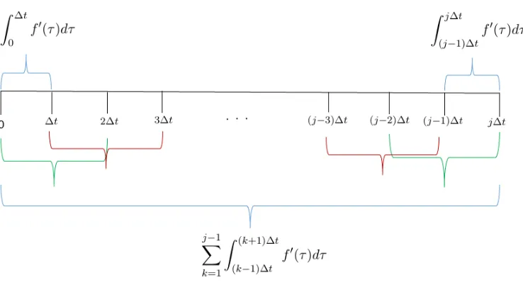
2.12 Intervals used to evaluate the integral in Equation (2.54). . . 41

2.13 (Color online) The value of Υ(j, p) in Equation (2.127) as shown versus p

(18)

LIST OF FIGURES xvi

2.14 (Color online) The absolute error found by using the C1 scheme to evaluate the fractional derivative of order p= 1−γ, where 0< γ≤ 1, of function

f(t) = t2 at time t = 1.0. The error is given for γ = 0.1, . . . ,0.9, where

γ increases in the direction of the arrow. Dashed lines show lines of slope 1 +γ for comparison. . . 60

2.15 (Color online) The value of the absolute error in using C1 scheme to ap-proximate the fractional derivative of order 1−γ for the functionf(t) =t3

at the time t= 1.0, with γ = 0.1, . . . ,0.9. The value of γ increases in the direction of the arrow and the dashed lines show lines of slope 1 +γ for comparison. . . 60

2.16 (Color online) The absolute error in using the C1 scheme to estimate the fractional derivative of order 1−γ for the functionf(t) =t4 shown at the time t= 1.0, forγ = 0.1, . . . ,0.9. The value of γ increases in the direction of the arrow. Dashed lines show lines of slope 1 +γ for comparison. . . . 61

2.17 (Color online) The absolute error in using the C1 scheme to evaluate the fractional derivative of order 1−γ for the functionf(t) = 1−et+t3, where

2.18 (Color online) The absolute error in using the C1 scheme to evaluate the fractional derivative of order 1−γ for the functionf(t) = 1 +tγ at the time

2.19 (Color online) The value of ˆϑ(j, γ) in Equation (2.151) is shown versuspfor varying number of time steps j= 10,102,103, . . . ,106, wherej increases in the direction of the arrow. These results show ˆϑ(j, γ) is bounded above by

1

(19)

LIST OF FIGURES xvii

2.20 (Color online) The absolute error, ε, in the C2 approximation of the frac-tional derivative of order 1−γ on the functionf(t) =t2 at the timet= 1.0 given for γ = 0.1,0.2,0.3. . . ,0.8,0.9. Note γ increases in the direction of the arrow, and dashed lines show lines of slope 1 +γ for comparison. . . . 69

2.21 (Color online) The absolute error in the C2 scheme approximation of the order 1−γ fractional derivative of the functionf(t) =t3shown at the time

t = 1.0 with γ = 0.1, . . . ,0.9. The value ofγ increases in the direction of the arrow, and for comparison we show lines of slope 1 +γ as a dashed lines. 70

2.22 (Color online) The absolute error found by using the C2 scheme approxi-mation of the fractional derivative of order 1−γ on the functionf(t) =t4

at the timet= 1.0, and forγ = 0.1, . . . ,0.9. The value ofγ increases in the direction of the arrow. Dashed lines show lines of slope 1 +γ for comparison. 70

2.24 (Color online) The absolute error in using the C2 scheme to evaluate the fractional derivative of order 1−γ for the functionf(t) = 1 +tγ at the time

2.25 (Color online) The value of K(j, p) in Equation (2.176) as shown versus

p for varying number of time steps are j = 10,102,103, . . . ,106, where

(20)

LIST OF FIGURES xviii

2.26 (Color online) The value of the absolute error found by using the C3 scheme to approximate the fractional derivative of order 1 −γ of the function

f(t) = t2 at time t = 1.0. The error is shown for γ = 0.1, . . . ,0.9, where the value of γ increases in the direction of the arrow, and the dashed lines show lines of slope 1 +γ for comparison. For small ∆tthe error is of order

O(∆t1+γ). . . 80 2.27 (Color online) The absolute error in the estimate of the C3 approximation

of the fractional derivative of order 1−γ of the function f(t) =t3 shown at t= 1.0. The error is shown for γ = 0.1, . . . ,0.9 with γ increases in the direction of the arrow. Dashed lines show lines of slope 1 +γ for comparison. 80

2.28 (Color online) The value of the absolute error in the estimate of the frac-tional derivative of order 1−γ for the function f(t) =t4 found by using the C3 approximation at the time t= 1.0, and for γ = 0.1, . . . ,0.9. Note the value of γ increases in the direction of the arrow. Dashed lines show lines of slope 1 +γ for comparison. . . 81

2.30 (Color online) The absolute error in using the C3 scheme to evaluate the fractional derivative of order 1−γ for the function f(t) = 1 +tγ at the time t = 1.0 with γ = 0.1, . . . ,0.9, and γ increases in the direction of the arrow. Dashed lines show lines of slope 1 +γ for comparison. . . 82

2.31 (Color online) The value of the absolute error found by using the RInt

(21)

LIST OF FIGURES xix

2.32 (Color online) The absolute error in the estimate of the RInt approxima-tion, Equation (2.191), found for the fractional derivative of the function

f(t) =t3 of order 1−γ att= 1.0. The error is shown forγ = 0.1, . . . ,0.9 with γ increases in the direction of the arrow and the dashed lines show lines of slope 1 +γ for comparison. . . 87

2.33 (Color online) The value of the absolute error of the fractional derivative of order 1−γ for the functionf(t) =t4 found by using theRInt approx-imation, Equations (2.191), at the time t = 1.0, and for γ = 0.1, . . . ,0.9. Note the value of γ increases in the direction of the arrow. Dashed lines show lines of slope 1 +γ for comparison. . . 88

2.34 (Color online) The absolute error in using theRIntapproximation, Equa-tions (2.191), to evaluate the fractional derivative of order 1−γ for the function f(t) = 1−et+t3, whereγ = 0.1, . . . ,0.9 and timet= 1.0. Note

γ increases in the direction of the arrow, and the dashed lines show lines of slope 1 +γ for comparison. . . 88

2.35 (Color online) The absolute error in using theRIntapproximation, Equa-tions (2.191), to evaluate the fractional derivative of order 1 −γ, where

γ = 0.1, . . . ,0.9, for the functionf(t) = 1 +tγ at the time t= 1.0. Note γ

increases in the direction of the arrow, and the dashed lines show lines of slope 1 +γ for comparison. . . 89

2.36 The value ofκ(1000, n, p) in Equation (2.240) is shown againstpfor varying values of n = 50l, where l = 1,2, . . . ,8. The value of n increases in the direction of the arrow. Note the value of κ(1000, n, p) increases as p, 0≤

p≤1, decreases. . . 104

2.37 The value ofκ(j,50, p) in Equation (2.240) is shown againstpfor 0≤p≤1 for fixed n = 50 and j = 10k where k = 2,3,4,5 and 6. The value of

(22)

LIST OF FIGURES xx

2.38 The maximum value of κ(j, j, p) in Equation (2.240) is shown against p

for 0 ≤p ≤ 1 for n= j = 1, . . . ,10. The value of κ(j, j, p) increases as j

increases in the direction of the arrow. . . 105

2.39 The absolute error in using the L1∗ scheme, Equation (2.194), for the fractional derivative of order 1−γof the functionf(t) =t2, at timet= 1.0, withj = 100 andn= 1, . . . , j. Results are shown forγ = 0.1, . . . ,0.9 where

γ increases in the direction of the arrow. . . 106

2.40 The absolute error in using the L1∗ scheme, Equation (2.194), for the fractional derivative of order 1 −γ of the function f(t) = t2.5, at time

t = 1.0, with j = 100 with n = 1, . . . ,100. Results are shown for γ = 0.1, . . . ,0.9 where γ increases in the direction of the arrow. . . 106

2.41 The absolute error in using the L1∗ scheme, Equation (2.194), to evaluate the fractional derivative of order 1−γ for function f(t) = t3, at time

t= 1.0. Results shown forj= 100, withn= 1, . . . ,100 forγ = 0.1, . . . ,0.9 where γ increases in the direction of the arrow. . . 107

2.42 The absolute error in using the L1∗ scheme, Equation (2.194), for the fractional derivative of order 1 −γ of the function f(t) = t3.5, at time

t = 1.0, with the time step j = 100 where n = 1, . . . ,100. Results are shown for γ = 0.1, . . . ,0.9 where γ increases in the direction of the arrow. 107

2.43 The absolute error in using the L1∗ scheme, Equation (2.194), to evaluate the fractional derivative of order 1−γfor functionf(t) =t4, at timet= 1.0. Results shown for j = 100, n= 1, . . . ,100, and for value γ = 0.1, . . . ,0.9 where γ increases in the direction of the arrow. . . 108

2.44 The value of_bκ(j, n, p) in Equation (2.273) is shown againstp, for 0≤p≤1, for varying number of n= 50l, wherel= 1,2, . . . ,8 and j= 1000. Note n

(23)

LIST OF FIGURES xxi

2.45 The value of_bκ(j, n, p) in Equation (2.273) is shown againstp, for 0≤p≤1, for fixed n = 50 and j = 10k where k = 2,3,4,5 and 6. The value of

b

κ(j, n, p) decreases asj increases in the direction of the arrow for fixedn. 116

2.46 The value of_bκ(j, n, p) in Equation (2.273) is shown againstp, for 0≤p≤1, for n=j= 1, . . . ,10. The value of bκ(j, j, p) increases as j increases in the

direction of the arrow. . . 117

2.47 The absolute error in using the RL1 scheme, in Equation (2.270), to approx-imate the fractional derivative of order 1−γof the functionf(t) =t2, at the timet= 1.0, usingj= 100 time steps,n= 1, . . . ,100 andγ = 0.1, . . . ,0.9. In the figure γ increases in the direction of the arrow. . . 118

2.48 The absolute error in using the RL1 scheme, Equation (2.270), to approx-imate the fractional derivative of order 1−γ of the function f(t) = t2.5, at the time t = 1.0, using 100 time steps for n = 1, . . . ,100 and γ = 0.1, . . . ,0.9. The value γ increases in the direction of the arrow. . . 118

2.49 The absolute error in using the RL1 scheme, in Equation (2.270), to evalu-ate the fractional derivative of order 1−γfor functionf(t) =t3, at the time

t= 1.0. Results are shown forj = 100,n= 1, . . . ,100 and γ = 0.1, . . . ,0.9 where γ increases in the direction of the arrow. . . 119

2.50 The absolute error in using the RL1 scheme, Equation (2.270), to approx-imate the fractional derivative of order 1−γ of the function f(t) = t3.5, at time t = 1.0, using 100 time steps and for n = 1, . . . ,100 and γ = 0.1, . . . ,0.9 where γ increases in the direction of the arrow. . . 119

2.51 The absolute error in using the RL1 scheme, in Equation (2.270), to eval-uate the fractional derivative of order 1−γ for functionf(t) =t4_{, at time}

(24)

LIST OF FIGURES xxii

2.52 The value of the absolute error in using the LRA scheme, Equation (2.279), to approximate the fractional derivative of order 1−γ of functionf(t) =t2, at time t= 1.0. The results are shownn= 1, . . . ,100 and γ = 0.1, . . . ,0.9 where γ increases in the direction of the arrow. . . 123

2.53 The value of the absolute error in using the LRA scheme, Equation (2.279), to estimate the fractional derivative of order 1−γ of functionf(t) =t2.5, at timet= 1.0. The results are shown forn= 1, . . . ,100 andγ = 0.1, . . . ,0.9 where γ increases in the direction of the arrow. . . 123

2.54 The value of the absolute error by using Equation (2.279), to evaluate the fractional derivative of order 1−γ of function f(t) =t3, at time t= 1.0,

n = 1, . . . ,100 and γ = 0.1, . . . ,0.9 where γ increases in the direction of the arrow. . . 124

2.55 The value of the absolute error by using Equation (2.279), to evaluate the fractional derivative of order 1−γ of function f(t) =t3.5, at time t= 1.0,

n = 1, . . . ,100 and γ = 0.1, . . . ,0.9 where γ increases in the direction of the arrow. . . 124

2.56 The value of the absolute error in using the LRA scheme, Equation (2.279), to evaluate the fractional derivative of order 1−γ of functionf(t) =t4, at time t= 1.0, n= 1, . . . ,100. Results are shown forγ = 0.1, . . . ,0.9 where

2.57 The value of the absolute error in using Equation (2.284) to evaluate the fractional derivative of order 1−γ of the function f(t) =t2 at time t= 1. The error increases as n increases for largen and the value of γ increases in the direction of the arrow. . . 128

2.58 The value of the absolute error in evaluating the fractional derivative of order 1−γ of the functionf(t) =t2.5 _at_t_{= 1 by using Equation (2.284).}

(25)

LIST OF FIGURES xxiii

2.59 The value of the absolute error in evaluating the fractional derivative of order 1−γ of the function f(t) = t3 att = 1 by using Equation (2.284). Note as n increases the error increases for large n and γ increases in the direction of the arrow. . . 129

2.60 The value of the absolute error in evaluating the fractional derivative of order 1−γ of the functionf(t) =t3.5 att= 1 by using Equation (2.284). Note as n increases the error increases for large n and the value of γ in-creases in the direction of the arrow. . . 129

2.61 The value of the absolute error in using Equation (2.284) to evaluate the fractional derivative of order 1−γ of the functionf(t) =t4at timet= 1, for largenthe error increases asnincreases. Noteγ increases in the direction of the arrow. . . 130

2.62 The value of the absolute error in using the NLRA scheme, Equation (2.291), to approximate the fractional derivative of order 1 −γ of the function

f(t) = t2 at time t= 1.0. Here 100 time steps were taken with nvarying from 1 to 100 and γ = 0.1, . . . ,0.9. The error increases as nincreases and the value of γ increases in the direction of the arrow. . . 133

2.63 The value of the absolute error in evaluating the fractional derivative of order 1 −γ of the function f(t) = t2.5, at time t = 1.0 by using Equation (2.291). The results are shown for j = 100, n = 1, . . . , j and

γ = 0.1, . . . ,0.9, and the error increase as n increases and the value of γ

increases in the direction of the arrow. . . 134

(26)

LIST OF FIGURES xxiv

2.65 The value of the absolute error in evaluating the fractional derivative of order 1 −γ of the function f(t) = t3.5, at time t = 1.0 by using Equation (2.291). The results are shown for j = 100, n = 1, . . . , j and

γ = 0.1, . . . ,0.9, and the error increase as nincreases. Note γ increases in the direction of the arrow. . . 135

2.66 The value of the absolute error in using Equation (2.291) to evaluate the fractional derivative of order 1−γof the functionf(t) =t4, at timet= 1.0. Results shown for 100 time steps, n= 1, . . . ,100 andγ = 0.1, . . . ,0.9 and

3.1 Geometric interpretation of the finite difference approximation of the time derivative. . . 149

3.2 Prediction of ζj/ζ0 found from numerically evaluating the recurrence

rela-tion in Equarela-tion (3.43). Results are shown for 100 time steps, λq = 1 and γ = 0.1, . . . ,0.9. In this figure γ increases in the direction of the arrow. . . 161

3.3 Results of ζj/ζj−1 found from Equation (3.43) forj = 1, . . . ,100, λq = 1

and γ = 0.1, . . . ,0.9. In this figure γ increases in the direction of the arrow. 162

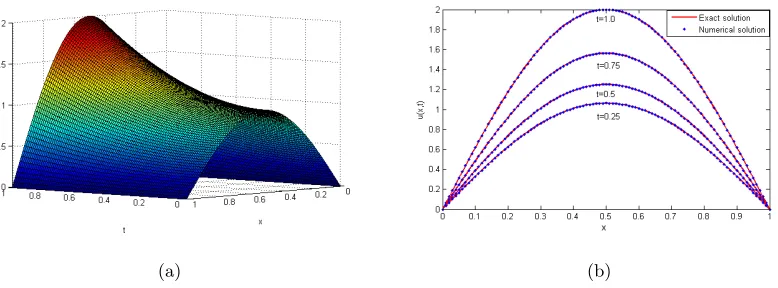
3.4 A comparison of the exact solution and the numerical solution of Equa-tion (3.142) shown at the times t= 0.25,0.5,0.7 and 1.0, for γ = 0.5, and time step ∆t= 10−3. . . 170 3.5 The numerical solution by the IMC1 scheme for Equation (3.142) shown

for 0≤t≤1, and 0≤x≤1 in the case γ = 0.5. . . 170

3.6 A comparison of the exact solution and the numerical solution for Equa-tion (3.145) at different timest= 0.25, 0.5, 0.75, and 1.0 withγ = 0.5 and ∆t= 10−3. . . 172 3.7 The numerical solution by the IMC1 scheme for Equation (3.145) for 0≤

(27)

LIST OF FIGURES xxv

3.8 A comparison of the exact solution and the numerical solution for Equa-tion (3.148) at times t = 0.25, 0.5, 0.75, and 1.0 in the case γ = 0.5 and ∆t= 10−4. . . 174 3.9 A comparison of the exact solution and the numerical solution present at

the mid point x = 0.5 for Equation (3.148) with γ = 0.5 and time step ∆t= 10−4. . . 174 3.10 The numerical solution of Equation (3.148), using the IMC1 scheme, shown

in the case of the fractional exponent (a) γ = 0.1, and (b)γ = 0.5 on the domain 0≤t≤1, and 0≤x≤1 with ∆t= 10−4. . . 175 3.11 The numerical solution of Equation (3.148), using the IMC1 scheme, shown

in the case of the fractional exponent (a) γ = 0.9, and (b) γ = 1 on the domain 0≤t≤1, and 0≤x≤1 with ∆t= 10−4. . . 175 4.1 The value of the ratio ζj/ζ0 predicted by evaluating Equation (4.33).

Re-sults are shown for 100 time steps, Vq = 4, and γ = 0.1, . . . ,0.9. Note the

value of γ increases in the direction of the arrow. . . 188

4.2 The value of the ratioζj/ζ0found from recurrence relation in Equation (4.33).

Results are shown for 100 time steps, Vq = 2, and γ = 0.1, . . . ,0.9. Note

the value of γ increases in the direction of the arrow. . . 188

4.3 The value of the ratio ζj/ζ0 predicted by evaluating Equation (4.33).

Re-sults are shown for 100 time steps, Vq = 1.5, andγ = 0.1, . . . ,0.9. . . 189

4.4 The value of the ratioζj/ζ0found from recurrence relation in Equation (4.33).

Results are shown for 100 time steps, Vq= 1, andγ = 0.1, . . . ,0.9. . . 189

(28)

LIST OF FIGURES xxvi

4.6 A comparison of the exact solution and the numerical solution present for equation (4.103) at the timest1 = 10−6, t2 = 0.75×10−6, t3 = 0.5×10−6,

and t4 = 0.25×10−6, withγ = 0.5 and ∆t1+γ/∆x2 = 10−10. . . 198

5.1 The grid points used in the Keller Box method (a) shows the grid points for the Box scheme, (b) the difference molecule for evaluationv_ij₋1

2

in equa-tion (5.4), and (c) the difference molecule for equaequa-tion (5.5). . . 201

5.2 The range of values of Λq and γ for both cases to be considered when

testing the stability of the KBMC2 scheme. . . 229

5.3 The predicted of ρ(γ, k,Λq) forγ = 0,0.1,0.2, . . . ,1,k= 1000 and Λq= 2γ. 233

5.4 Case 2 the predicted ratios ζj/ζ0 from Equation (5.169), with ζ0 = 1,

for various of γ is shown for Λq = 1/eµ0(γ). Note the ratios ζj/ζ0 for j = 1, . . . ,5 and log₃2≤γ ≤1 are bounded above by 1 and below by −1. The ratios for γ = 0.1,0.2, . . . ,1 decay to zero. Arrows show the direction of increasing γ. . . 234

5.5 Case 2 the predicted ratios ζj/ζ0 from Equation (5.169), with ζ0 = 1 for

various ofγ is shown for Λq= 2γ. Note the ratiosζj/ζ0forj= 1, . . . ,5 and

log₃2 ≤ γ ≤1 are bounded above by 1 and below by −1. The ratios for

γ = 0.1,0.2, . . . ,1 decay to zero. Arrows show the direction of increasing γ. 234

5.6 Ratios ζj/ζ0 predicted by Equation (5.169) with ζ0 = 1 for various of γ in

Case 2 where Λq = 2log32, j= 1, . . . ,4 and log32≤γ ≤1, the magnitude

of the ratios is less than 1. The arrows show the direction of increasing γ. 235

5.7 The predictions from Equation (5.169) of the ratio ζj/ζ0 with ζ0 = 1 for

various of γ is shown for Case 1 where Λq = 1, j = 1, . . . ,100 and γ =

0,0.1,0.2, . . . ,1 . The arrow shows the direction of increasing γ. . . 235

(29)

LIST OF FIGURES xxvii

5.9 The predictions of the ratioζj/ζ0found from Equation (5.247), withζ0 = 1.

Results are shown for Case 1, where j = 1, . . . ,6, γ = 0.1, . . . ,0.9 and ˘

Λq= 1. Note the ratios ζj/ζ0 is less than 1 where the value of γ decreases

in the direction of the arrow. . . 247

5.10 The predictions from Equation (5.247) of the ratio ζj/ζ0 with ζ0 = 1 is

shown for Case 2, where ˘Λq= 2. Note the ratiosζj/ζ0 forj= 1, . . . ,7, and

γ = 0.1, . . . ,0.9 is less than 1 and the value ofγ decreases in the direction of the arrow. . . 248

5.11 The predictions from Equation (5.247) of the ratio ζj/ζ0 with ζ0 = 1 is

shown for Case 2, where ˘Λq= 21−γ. Note the ratiosζj/ζ0 forj = 1, . . . ,6,

and γ = 0.1, . . . ,0.9. The value of γ decreases in the direction of the arrow. 248

5.12 The ratio ζj/ζ0 predictions from Equation (5.275) with ζ0 = 1 for γ =

0.1, . . . ,0.9 and ˆΛq = 1. Note the ratios ζj/ζ0 remain less than 1. The

value of γ decreases in the direction of the arrow. . . 252

5.13 The ratio ζj/ζ0 predictions from Equation (5.275), with ζ0 = 1, for γ =

0.1, . . . ,0.9 and ˆΛq = 1/2. Note the ratios ζj/ζ0, for j = 1, . . . ,100 and

0< γ≤1, remain less than 1. The value ofγ decreases in the direction of the arrow. . . 252

5.14 Numerical results of applying the KBMC2 method to solve Equation (5.453) in the case γ = 0.5. In (a) the numerical solution u(x, t) is given for 0 ≤t≤1 and 0 ≤x≤1, and in (b) the exact solution (red line) is com-pared with the approximation solution(blue dots) at the times t = 0.25, 0.50, 0.75, and 1. . . 282

(30)

LIST OF FIGURES xxviii

5.16 Numerical results of applying the KBMC3 method to solve Equation (5.453) in the case γ = 0.5. In (a) the numerical solution u(x, t) is given for 0 ≤t≤1 and 0 ≤x≤1, and in (b) the exact solution (red line) is com-pared with the approximation solution (blue dots) at the times t = 0.25, 0.50, 0.75, and 1. . . 283

5.17 Numerical results of applying the KBMC3 method to solve Equation (5.453) in the caseγ= 1. In (a) the numerical solutionu(x, t) is given for 0≤t≤1 and 0 ≤x ≤1, and in (b) the exact solution (red line) is compared with the approximation solution (blue dots) at the times t = 0.25, 0.50, 0.75, and 1. . . 283

5.18 Numerical results of applying the KBML1 method to solve Equation (5.453) in the case γ = 0.5. In (a) the numerical solution u(x, t) is given for 0 ≤t≤1 and 0 ≤x≤1, and in (b) the exact solution (red line) is com-pared with the approximation solution (blue dots) at the times t = 0.25, 0.50, 0.75, and 1. . . 284

5.19 Numerical results of applying the KBML1 method to solve Equation (5.453) in the caseγ= 1. In (a) the numerical solutionu(x, t) is given for 0≤t≤1 and 0 ≤x ≤1, and in (b) the exact solution (red line) is compared with the approximation solution (blue dots) at the times t = 0.25, 0.50, 0.75, and 1. . . 284

5.20 Numerical results of applying the KBMC2-FADE method to solve Equa-tion (5.454) in the case γ = 0.5. In (a) the numerical solution u(x, t) is given for 0 ≤ t ≤ 1 and 0 ≤ x ≤ 1, and in (b) the exact solution (red line) is compared with the approximation solution (blue dots) at the times

(31)

LIST OF FIGURES xxix

5.21 Numerical results of applying the KBMC2-FADE method to solve Equa-tion (5.454) in the case γ = 1. In (a) the numerical solution u(x, t) is given for 0 ≤ t ≤ 1 and 0 ≤ x ≤ 1, and in (b) the exact solution (red line) is compared with the approximation solution (blue dots) at the times

t= 0.25, 0.50, 0.75, and 1. . . 285

5.23 Numerical results of applying the KBMC2 method to solve Equation (5.457) in the caseγ= 1. In (a) the numerical solutionu(x, t) is given for 0≤t≤1 and 0 ≤x ≤1, and in (b) the exact solution (red line) is compared with the approximation solution (blue dots) at the times t = 0.25, 0.50, 0.75, and 1. . . 290

(32)

LIST OF FIGURES xxx

5.26 Numerical results of applying the KBML1 method to solve Equation (5.457) in the case γ = 0.5. In (a) the numerical solution u(x, t) is given for 0 ≤t≤1 and 0 ≤x≤1, and in (b) the exact solution (red line) is com-pared with the approximation solution (blue dots) at the times t = 0.25, 0.50, 0.75, and 1. . . 291

5.27 Numerical results of applying the KBML1 method to solve Equation (5.457) in the caseγ= 1. In (a) the numerical solutionu(x, t) is given for 0≤t≤1 and 0 ≤x ≤1, and in (b) the exact solution (red line) is compared with the approximation solution (blue dots) at the times t = 0.25, 0.50, 0.75, and 1. . . 292

5.28 Numerical results of applying the KBMC2-FADE method to solve Equa-tion (5.458) in the case γ = 0.5. In (a) the numerical solution u(x, t) is given for 0 ≤ t ≤ 1 and 0 ≤ x ≤ 1, and in (b) the exact solution (red line) is compared with the approximation solution (blue dots) at the times

t= 0.25, 0.50, 0.75, and 1. . . 292

5.29 Numerical results of applying the KBMC2-FADE method to solve Equa-tion (5.458) in the case γ = 1. In (a) the numerical solution u(x, t) is given for 0 ≤ t ≤ 1 and 0 ≤ x ≤ 1, and in (b) the exact solution (red line) is compared with the approximation solution (blue dots) at the times

t= 0.25, 0.50, 0.75, and 1. . . 293

5.30 A comparison of the exact solution and the numerical solution, using the KBMC2 scheme, for Equation (5.461) shown at times t = 0.25, 0.5, 0.75, and 1.0 in the caseγ = 0.5 and ∆t= 10−4. Time increases in the direction of arrow. . . 294

(33)

LIST OF FIGURES xxxi

5.32 A comparison of the exact solution and the numerical solution, using the KBML1 scheme, for Equation (5.461) shown at times t= 0.25, 0.5, 0.75, and 1.0 in the caseγ = 0.5 and ∆t= 10−4. Time increases in the direction of arrow. . . 295

5.33 A comparison of the exact solution and the numerical solution, using the KBMC2 scheme, present at the mid point x = 0.5 for Equation (5.461) with γ = 0.5 and time step ∆t= 10−4. . . 295 5.34 A comparison of the exact solution and the numerical solution, using the

KBMC3 scheme, present at the mid point x = 0.5 for Equation (5.461) with γ = 0.5 and time step ∆t= 10−4. . . 296 5.35 A comparison of the exact solution and the numerical solution, using the

KBML1 scheme, present at the mid point x = 0.5 for Equation (5.461) with γ = 0.5 and time step ∆t= 10−4. . . 296 5.36 The numerical solution of Equation (5.461) using the KBMC2 scheme

shown here in the case of the fractional exponent (a) γ = 0.1, and (b)

γ = 0.5 on the domain 0≤t≤1, and 0≤x≤1 using with ∆t= 10−4. . . 297 5.37 The numerical solution of Equation (5.461) using the KBMC2 scheme

γ = 1 on the domain 0≤t≤1, and 0≤x≤1 using with ∆t= 10−4. . . . 297 5.38 The numerical solution of Equation (5.461) using the KBMC3 scheme

γ = 0.5 on the domain 0≤t≤1, and 0≤x≤1 using with ∆t= 10−4_{. . .} ₂₉₈

5.39 The numerical solution of Equation (5.461) using the KBMC3 scheme shown here in the case of the fractional exponent (a) γ = 0.9, and (b)

(34)

LIST OF FIGURES xxxii

5.40 The numerical solution of Equation (5.461) using the KBML1 scheme shown here in the case of the fractional exponent (a) γ = 0.1, and (b)

γ = 0.5 on the domain 0≤t≤1, and 0≤x≤1 using with ∆t= 10−4. . . 299 5.41 The numerical solution of Equation (5.461) using the KBML1 scheme

γ = 1 on the domain 0≤t≤1, and 0≤x≤1 using with ∆t= 10−4. . . . 299 5.42 A comparison of the exact solution and the numerical solution for

Equa-tion (5.464), using the KBMC2–FADE scheme, shown at times t = 0.25, 0.5, 0.75, and 1.0 in the case γ = 0.5 and ∆t = 10−4. Time increases in the direction of arrow. . . 300

5.43 A comparison of the exact solution and the numerical solution present at the mid point x = 0.5 for Equation (5.464), using the KBMC2-FADE scheme, with γ = 0.5 and time step ∆t= 10−4. . . 301 5.44 The numerical solution of Equation (5.464) using the KBMC2–FADE scheme

γ = 0.5 on the domain 0≤t≤1, and 0≤x≤1 using with ∆t= 10−4. . . 301 5.45 The numerical solution of Equation (5.464) using the KBMC2–FADE scheme

shown here in the case of the fractional exponent (a)γ = 0.9, and (b)γ = 1 on the domain 0≤t≤1, and 0≤x≤1 using with ∆t= 10−4. . . 302 6.1 Numerical solution for ODE, where k1 = 1,k−1= 1 and timet∈[0,10]. . 342

6.2 Numerical solution for ODE, where k1 = 1,k−1= 3 and timet∈[0,10]. . 343

6.3 Numerical solution for ODE, where k1 = 3,k−1= 1 and timet∈[0,10]. . 343

6.4 The predictions of A(x, t) given by the KBMC2 scheme, Section 6.3.1, for Model Type 1. . . 345

(35)

LIST OF FIGURES xxxiii

6.6 The Model Type 1 predictions of C(x, t) using the KBMC2 scheme, Sec-tion 6.3.1. . . 346

6.7 The Model Type 2 predictions of A(x, t) using the KBMC2 scheme, Sec-tion 6.6.1. . . 346

6.8 The predictions of B(x, t) using the KBMC2 scheme in Section 6.6.1 for Model Type 2. . . 347

6.9 The Model Type 2 predictions of C(x, t) using the KBMC2 scheme, Sec-tion 6.6.1. . . 347

6.10 The comparison between Model Type 1 and Model Type 2 by using KBMC2 for species A in Equations (6.14) and (6.95) at x = 0.5 (upper two lines) and 0.9 (lower two lines). . . 348

6.11 The estimate of the difference, , in the prediction for A(0.5, t) given by Model Type 1, and Model Type 2 by using KBMC2 for Equations (6.14) and (6.95) where =A1(0.5, t)−A2(0.5, t). . . 348

6.12 The Model Type 1 predictions ofA(x, t) using the IML1 scheme. . . 349

6.13 The Model Type 1 predictions ofB(x, t) using the IML1 scheme. . . 349

6.14 The Model Type 1 predictions ofC(x, t) using the IML1 scheme. . . 350

6.15 The Model Type 2 predictions ofA(x, t) using the IML1 scheme. . . 350

6.16 The Model Type 2 predictions ofB(x, t) using the IML1 scheme. . . 350

6.17 The Model Type 2 predictions ofC(x, t) using the IML1 scheme. . . 351

6.18 The estimate of the difference, , in the prediction for A(0.5, t) given by Model Type 2 with KBMC2, where1 is the difference between when ∆t=

10−2and ∆t= 10−3time steps,2 is the difference between ∆t= 10−3 and

∆t = 10−4 time steps. The value 3 is the difference between ∆t= 10−4

(36)

LIST OF FIGURES xxxiv

6.19 The estimate of the difference, , in the prediction for C(0.5, t) given by Model Type 2 with KBMC2, where1 is the difference between when ∆t=

and ∆t= 10−5 time steps. . . 353 6.20 The estimate of the difference, , in the prediction for A(0.5, t) given by

Model Type 1 with KBMC2, where1 is the difference between when ∆t=

and ∆t= 10−5 time steps. . . 354 6.21 The estimate of the difference, , in the prediction for C(0.5, t) given by

Model Type 1 with KBMC2, where1 is the difference between when ∆t=

and ∆t= 10−5 time steps. . . 354 6.22 The comparison between the KBMC2 scheme and the IML1 scheme for

Model Type 2 (species A) at x= 0.5 with 0≤t≤1. . . 358

6.23 The comparison between the KBMC2 scheme and the IML1 scheme for Model Type 2 (species A) at x= 0.3 (upper two lines) and 0.9 (lower two lines), with 0≤t≤1. . . 358

6.24 The Model Type 1 predictions of C(x, t) using the KBMC2 scheme, Sec-tion 6.6.1, where k1= 0, andk−1 = 2. . . 360

6.25 The Model Type 2 predictions of C(x, t) using the the KBMC2 scheme, Section 6.3.1, where k1 = 0, andk−1= 2. . . 360

6.26 Comparison between Model Type 1 and Model Type 2 predictions for

C(0.1, t) by using the KBMC2 scheme for γ = 0.5, with ∆t = 0.001,

(37)

LIST OF FIGURES xxxv

6.27 Comparison between Model Type 1 and Model Type 2 predictions for

C(0.9, t) by using the KBMC2 scheme for γ = 0.5, with ∆t = 0.001,

k1 = 0, andk−1 = 2. . . 361

B.1 Plot of functions f1(τ) and f2(τ) showing f1(τ) ≥ f2(τ) over the range

τ ∈[tl, tl+1]. . . 382

B.2 Plot of functions in the terms in the first integrand (a)f1(τ) andf2(τ), and

the term in the second integrand (b) f1(τ) and f3(τ) of Equation (2.145).

Note f1(τ)≥f2(τ) and f1(τ)≥f3(τ) over the range ofτ plotted. . . 393

B.3 The range of values ofa and b for all cases to be considered when testing the bound of Equation (B.111) . . . 406

B.4 Bound of y1, wherey1 = 1 +x(1−3γ) with 0< γ≤1 and 0≤x≤1. . . 409

(38)

List of Tables

2.1 The comparison of the absolute error in evaluating the fractional derivative of order 1−γ for the functions f(t), Equation (2.7), at time t = 1.0 by using the GL scheme where γ = 0.1, ...,0.9 and ∆t= 0.01. . . 27

2.2 The comparison of the absolute error in the L1 approximation of the frac-tional derivative of order p = 1−γ of the function f(t), given by Equa-tion (2.7), at time t= 1.0 where γ = 0.1, ...,0.9 and ∆t= 0.01. . . 39

2.3 Numerical accuracy in ∆tof the L1 scheme applied to the functionf(t) = 1 +tγ, andRb is order of convergence. . . 40

2.4 The comparison of the absolute error in the C1 scheme estimate of the frac-tional derivative of order p= 1−γ of the functionsf(t) in Equation (2.7) at the time t= 1.0 with γ = 0.1, ...,0.9 and ∆t= 0.01. . . 62

2.5 Numerical accuracy in ∆tof the C1 scheme applied to the functionf(t) = 1 +tγ, whereRb is order of convergence. . . 63

2.6 The comparison of the absolute error in the estimate of the fractional derivative of order p= 1−γ by using the C2 scheme on the functionsf(t) in Equation (2.7) at the time t= 1.0 where γ = 0.1, ...,0.9 and ∆t= 0.01. 72

(39)

LIST OF TABLES xxxvii

2.8 The comparison of the absolute error in the estimate of the order 1−γ

fractional derivative of the functions f(t), Equation (2.7), at time t= 1.0 where γ = 0.1, ...,0.9 and ∆t= 0.01 by using the C3 approximation. . . . 82

2.9 Numerical accuracy in ∆tof the C3 scheme applied to the functionf(t) = 1 +tγ, andRb is order of convergence. . . 83

2.10 The comparison of the absolute error in the estimate of the fractional derivative of order 1 −γ on the functions f(t), Equation (2.7), at the time t= 1.0 with γ = 0.1, ...,0.9 and ∆t= 0.01 by using theRInt scheme approximation. . . 89

2.11 Numerical accuracy in ∆t of the RInt scheme applied to the function

f(t) = 1 +tγ, whereRb is order of convergence. . . 90

2.12 The comparison of the absolute error for functionsf(t) =tk,k= 2,2.5,3,3.5, and 4 at time t= 1.0 with n= 100, j= 100, and ∆t= 0.01 using the L1∗ scheme to evaluate the 1−γ order fractional derivative, whereγ = 0.1, ...,0.9.108

2.13 The comparison of the absolute error in the RL1 approximate estimate of the fractional derivative of order 1−γ of the functions f(t) = tk, k = 2,2.5,3,3.5, and 4 at time t= 1.0 whereγ = 0.1, ...,0.9,n= 100,j = 100 and ∆t= 0.01. . . 120

2.14 The comparison of the absolute error in the LRA scheme estimate of the fractional derivative of order 1−γ of the functions f(t) = tk_, _k ₌

2,2.5,3,3.5, and 4 at the timet= 1.0 forγ = 0.1, ...,0.9,n= 100,j = 100, and ∆t= 0.01. . . 125

(40)

LIST OF TABLES xxxviii

2.16 The comparison minimum absolute error in the QRA scheme estimate of the fractional derivative of order 1−γ of the functions f(t) = tk, k = 2,2.5,3,3.5, and 4 at the time t = 1.0 for γ = 0.1, ...,0.9, j = 100, and ∆t= 0.01. . . 131

2.17 The comparison of the absolute error in the estimate of the fractional derivative of order 1−γ using the NLRA scheme on the functionsf(t) =tk,

k = 2,2.5,3,3.5, and 4 at the time t = 1.0 for γ = 0.1, ...,0.9, n = 100,

j = 100, and ∆t= 0.01. . . 136

2.18 The comparison minimum absolute error in the NLRA scheme estimate of the fractional derivative of order 1−γ of the functions f(t) =tk, k= 2,2.5,3,3.5, and 4 at the time t = 1.0 for γ = 0.1, ...,0.9, j = 100, and ∆t= 0.01. . . 136

2.19 The comparison absolute error of the fractional derivative approximation of order 1−γ of function f(t) =t2 at time t= 1.0 for γ = 0.1, ...,0.9 and ∆t= 0.01. . . 138

2.22 The comparison absolute error of the fractional derivative approximation of order 1−γ of functionf(t) = 1−et+t3at timet= 1.0 forγ = 0.1, ...,0.9 and ∆t= 0.01. . . 139

(41)

LIST OF TABLES xxxix

2.24 The comparison absolute error of the fractional derivative approximation of order 1−γ of the functionf(t) =t2 at time t= 1.0 for γ = 0.1, ...,0.9,

n= 100, j= 100, and ∆t= 0.01. . . 141

n= 100, j= 100 and ∆t= 0.01. . . 141

2.26 The comparison absolute error of the fractional derivative approximation of order 1−γ of the function f(t) = t4 at time t= 1 for γ = 0.1, ...,0.9,

n= 100, j= 100 and ∆t= 0.01. . . 142

n= 50,j = 100, and ∆t= 0.01. . . 142

n= 50,j = 100 and ∆t= 0.01. . . 143

2.30 The comparison minimum absolute error of the fractional derivative ap-proximation of order 1−γ of the function f(t) = t2 _{at time} _t _{= 1}_._{0 for}

γ = 0.1, ...,0.9, j= 100, and ∆t= 0.01. . . 144

2.31 The comparison minimum absolute error of the fractional derivative ap-proximation of order 1−γ of the function f(t) = t3 at time t = 1.0 for

γ = 0.1, ...,0.9, j= 100 and ∆t= 0.01. . . 144

2.32 The comparison minimum absolute error of the fractional derivative ap-proximation of order 1−γ of the function f(t) = t4 at time t = 1.0 for

(42)

LIST OF TABLES xl

3.1 Numerical accuracy in ∆x of the IMC1 scheme applied to Example 3.7.1 with ∆t= 10−3 and R1 is order of convergence. . . 169 3.2 Numerical accuracy in ∆t of the IMC1 scheme applied to Example 3.7.1

with ∆x= 10−3 and R2 is order of convergence. . . 169 3.3 Numerical accuracy in ∆x of the IMC1 scheme applied to Example 3.7.2

with ∆t= 10−3 and R1 is order of convergence. . . 171 3.4 Numerical accuracy in ∆t of the IMC1 scheme applied to Example 3.7.2

with ∆x= 10−3 and R2 is order of convergence. . . 171 3.5 Numerical accuracy in ∆tand ∆x applied to Example 3.7.3 with γ = 0.5. 175

3.6 Numerical accuracy in ∆tand ∆x applied to Example 3.7.3 with γ = 1. . 176

4.1 Numerical accuracy in ∆x of the Dufort–Frankel scheme, Equation (4.8), with ∆t= 10−5∆x and R1 is order of convergence. . . 195 4.2 Numerical accuracy in ∆x of the Dufort–Frankel scheme, Equation (4.8),

with ∆t= 10−5∆x2 and R1 is order of convergence. . . 196 4.3 Numerical accuracy in ∆x of the Dufort–Frankel scheme, Equation (4.8),

with ∆t= 10−5∆x3 and R1 is order of convergence. . . 196 4.4 Numerical accuracy in ∆x of the Dufort–Frankel scheme, Equation (4.8),

with ∆t= 10−6_∆_x _and _R_{1 is order of convergence. . . .} ₁₉₇

4.5 Numerical accuracy in ∆x of the Dufort–Frankel scheme, Equation (4.8), with ∆t= 10−6∆x2 and R1 is order of convergence. . . 197 4.6 Numerical accuracy in ∆x of the Dufort–Frankel scheme, Equation (4.8),

with ∆t= 10−6∆x3 and R1 is order of convergence. . . 198 5.1 Numerical accuracy in ∆xof the KBMC2 scheme applied to Example 5.8.1

(43)

LIST OF TABLES xli

5.2 Numerical accuracy in ∆tof the KBMC2 scheme applied to Example 5.8.1 with ∆x= 10−3, whereR2 is the order of convergence in ∆t. . . 279 5.3 Numerical accuracy in ∆xof the KBMC3 scheme applied to Example 5.8.1

with ∆t= 10−3, and R1 is the order of convergence in ∆x. . . 279 5.4 Numerical accuracy in ∆tof the KBMC3 scheme applied to Example 5.8.1

with ∆x= 10−3, whereR2 is the order of convergence in ∆t. . . 280 5.5 Numerical accuracy in ∆xof the KBML1 scheme applied to Example 5.8.1

where ∆t= 10−3, and R1 is the order of convergence in ∆x. . . 280 5.6 Numerical accuracy in ∆tof the KBML1 scheme applied to Example 5.8.1

with ∆x= 10−3, whereR2 is the order of convergence in ∆t. . . 280 5.7 Numerical accuracy in ∆xof the KBMC2-FADE scheme applied to

Exam-ple 5.8.1 with ∆t= 10−3, and R1 is the order of convergence in ∆x. . . . 281 5.8 Numerical accuracy in ∆tof the KBMC2-FADE scheme applied to

Exam-ple 5.8.1, where ∆x= 10−3, and R2 is the order of convergence in ∆t. . . 281 5.9 Numerical accuracy in ∆xof the KBMC2 scheme applied to Example 5.8.2

where ∆t= 10−3, and R1 is the order of convergence in ∆x . . . 286 5.10 Numerical accuracy in ∆tof the KBMC2 scheme applied to Example 5.8.2

with ∆x= 10−3, whereR2 is the order of convergence in ∆t. . . 286 5.11 Numerical accuracy in ∆xof the KBMC3 scheme applied to Example 5.8.2

with ∆t= 10−3_{, and} _R_{1 is the order of convergence in ∆}_x_. _{. . . .} ₂₈₇

5.12 Numerical accuracy in ∆tof the KBMC3 scheme applied to Example 5.8.2 with ∆x= 10−3, and R2 is the order of convergence in ∆t. . . 287 5.13 Numerical accuracy in ∆xof the KBML1 scheme applied to Example 5.8.2,

(44)

LIST OF TABLES xlii

5.14 Numerical accuracy in ∆tof the KBML1 scheme applied to Example 5.8.2 with ∆x= 10−3, and R2 is the order of convergence in ∆t. . . 288 5.15 Numerical accuracy in ∆xof the KBMC2-FADE scheme applied to

Exam-ple 5.8.2 with ∆t= 10−3, and R1 is the order of convergence in ∆x. . . . 288 5.16 Numerical accuracy in ∆tof the KBMC2-FADE scheme applied to

Exam-ple 5.8.2 with ∆x= 10−3, and R2 is the order of convergence in ∆t. . . . 288 6.1 Numerical convergence order in ∆tfor Model Type 2 based of the KBMC2

scheme for species A(x, t), andR1 is order of convergence. . . 355

6.2 Numerical convergence order in ∆xfor Model Type 2 based of the KBMC2 scheme for species A(x, t), andR2 is order of convergence. . . 355

6.3 Numerical convergence order in ∆tfor Model Type 1 based of the KBMC2 scheme for species A(x, t), andR1 is order of convergence. . . 355

6.4 Numerical convergence order in ∆xfor Model Type 1 based of the KBMC2 scheme for species A(x, t) , and R2 is order of convergence. . . 356

6.5 Numerical convergence order in ∆tfor Model Type 2 based of the KBMC2 scheme for species C(x, t), andR1 is order of convergence. . . 356

6.6 Numerical convergence order in ∆xfor Model Type 2 based of the KBMC2 scheme for species C(x, t), andR2 is order of convergence. . . 356

6.7 Numerical convergence order in ∆tfor Model Type 1 based of the KBMC2 scheme for species C(x, t), andR1 is order of convergence. . . 357

(45)

Notation

Notation used in this thesis.

Chapter 1

γ The anomalous diffusion exponent.

Kγ Anomalous diffusion coefficient.

D, K1,γ Diffusion coefficient.

f(x, t) Source function.

g(x) Initial condition.

ϕ1(t), ϕ2(t) Fixed (Dirchlet) boundary conditions.

k1 Forward reaction rate.

k−1 Reverse reaction rate.

A(x, t), B(x, t),C(x, t) Concentrations of each chemical species.

(46)

Notation xliv

Chapter 2

p The fractional derivative order.

νl Scaled weights for the L1 scheme.

Al(p),Bl(p),αj(p), βj∗(p), µ∗j(p), Scaled weights for the C1 scheme.

e

βj(p),µej(p),νel Scaled weights for the C2 scheme.

b

αj(p),βb_j(p),µ_b_j(p),ν_b_l Scaled weights for the C3 scheme.

ϑ(j, p) Error bound coefficient for the L1 scheme.

Υ(j, p) Error bound coefficient for the C1 scheme.

ˆ

ϑ(j, p) Error bound coefficient for the C2 scheme.

K(j, p) Error bound coefficient for the C3 scheme.

b

R Approximate order of convergence in ∆t.

ζ(s, a) The Hurwitz Zeta function.

Mn Maximum absolute value of the second derivative.

ℵj(p) Scaled weights for theL1∗ scheme.

~j(p),ℵj(p) Scaled weights for the RL1 scheme.

k(j, n, p) Error bound coefficient for theL1∗ scheme.

b

k(j, n, p) Error bound coefficient for the RL1 scheme.

C,C∗ Accuracy coefficients.

β0, β1, β2 Fitting parameters of the regression line.

Is(p, q) The Incomplete Beta function.

(47)

Notation xlv

Chapter 3

γ Anomalous diffusion exponent.

ρ Diffusion coefficient.

xi Spatial grid points.

tj Temporal grid points.

aj, βj∗(γ), µ∗j(γ) Scaled weights for the IMC1 scheme.

ui Approximate solution.

Ui Exact solution.

A∗ Tridiagonal matrix.

τi,j Scaled truncation error.

ζj Von Neumann stability variable.

i Numerical error.

λq Stability constant.

$j(γ) Stability weight.

R1 Approximate order of convergence in ∆x.

R2 Approximate order of convergence in ∆t.

Chapter 4

σ Diffusion coefficient.

A Tridiagonal matrix.

aj, βj(γ), µj(γ) Scaled weights.

Ui Exact solution.

τi,j Scaled truncation error.

ζj Von Neumann stability variable.

i Numerical error.

(48)

Notation xlvi

Chapter 5

d, d1,d2 Diffusion coefficients.

Ui, Vi Exact solution.

e

βj(γ),µej(γ) Scaled weights for the KBMC2 scheme. κj(γ),αbj(γ),βbj(γ),µbj(γ) Scaled weights for the KBMC3 scheme. βj(γ), µj(γ) Scaled weights for the KBML1 scheme. τ_i,j(1),τ_i,j(2),τ_i,j(3) Scaled truncation errors.

M(t) Maximum absolute value of the fourth derivative in space.

ζj, ξj Von Neumann stability variables.

i, εi Numerical errors.

Λq,Λ˘q,Λˆq, Uq Stability constants. ρ(γ, k,Λq),ρ˘(γ, k,Λ˘q) Stability bound.

e

(49)

Notation xlvii

Chapter 6

A(x, t), B(x, t),C(x, t) Concentration Chemical species.

k1 Forward reaction rate.

k−1 Reverse reaction rate.

L1_t−γ Non-standard/modified fractional derivative operator.

d, dˆ Diffusion coefficients.

yk(x, t),k= 1,2,3 Auxiliary functions for Model Type 2.

e

βj(γ),µej(γ) Scaled weights for the KBMC2 scheme. βj(γ), µj(γ) Scaled weights for the IML1 scheme.

(50)

Acronyms & Abbreviations

L1 L1 approximation scheme.

GL Gr¨unwald-Letnikov approximation scheme.

C1 First modified L1 approximation scheme.

C2 Second modified L1 approximation scheme.

C3 Third modified L1 approximation scheme.

RInt Romberg Integration scheme.

RL1 Reduction of the L1 approximation scheme.

LRA Linear Regression Approximation scheme.

QRA Quadratic Regression Approximation scheme.

N LRA Nonlinear Regression Approximation scheme.

IM C1 Implicit finite difference method with the C1 scheme.

IM L1 Implicit finite difference method with the L1 scheme.

DF L1 Dufort–Frankel method with the L1 scheme.

KBM C2 Keller Box method with the C2 scheme.

KBM C3 Keller Box method with the C3 scheme.

KBM L1 Keller Box method with the L1 scheme.

(51)

Chapter 1

Introduction and Literature

Review

1.1

Background

Anomalous subdiffusion is a physical phenomenon which is observed in many systems which involving trapping, binding or macromolecular crowding. In recent years, exam-ples of anomalous diffusion have been discovered in many different fields such as fluid me-chanics (Chen, Wei, Sui, Zhang & Zheng 2011, Elbeleze, Kılı¸cman & Taib 2013), physics (Metzler & Klafter 2000b), engineering, and biology (Atangana & Alabaraoye 2013, Roul 2013). Anomalous diffusion is characterised by the asymptotic long-time behaviour of the mean-squared displacement of the form

h∆x2(t)i ∼ 2Kγ

Γ(1 +γ)∆t

γ _(1.1)

whereγ is the anomalous diffusion exponent andKγis the anomalous diffusion coefficient.

(52)

1.2 Different types of Fractional Derivatives 2

Mura 2008) and by using Fractional Partial Differential Equations (FPDEs) (Metzler & Klafter 2000b).

A Fractional Partial Differential Equation is a partial differential equation, which involves a temporal fractional derivative or spatial fractional derivative. For example one of the well-known FPDEs is the fractional subdiffusion equation, which has the form

∂f(x, t)

∂t = ∂1−γ ∂t1−γ

∂2f(x, t)

∂x2

, (1.2)

where the anomalous exponentγ lies in the interval 0< γ <1.

Another example is the fractional superdiffusion equation, which has the form:

∂f(x, t)

∂t =K

∂β_f₍_{x, t}₎

∂|x|β , (1.3)

where the exponentβ lies in the range 1< β <2. In Equations (1.2) and (1.3), _∂t∂11−γ−γ and

∂β

∂|x|β are fractional partial derivatives of temporal and spatial type respectively. Baeumer, Kov´acs & Meerschaert (2007) considered the fractional superdiffusion equation by extend-ing the Reproduction–Dispersal equations, where the second derivative in a diffusion or dispersion model is replaced by a fractional derivative of order 1< β <2.

A fractional derivative is an extension of the familiar derivative operator ∂n_∂tfn(t) by re-placing the integer valuen with a non-integer parameterpwhich can also be denoted as

∂p_f₍_t₎

∂tp orD

p

tf(t) (Samko, Kilbas & Marichev 1993, Podlubny 1998). Definitions of several

common fractional derivatives are given in the next section.

1.2

Different types of Fractional Derivatives

There are several definitions of fractional derivatives of the orderp, the Riemann–Liouville fractional derivative, the Caputo fractional derivative, the Gr¨unwald–Letnikov fractional derivative and the Riesz fractional derivative (Gorenflo & Mainardi 1998, Podlubny 1998, Li & Zeng 2015). Note p can also defined as a complex number or variable, but in this research we focus on p being a real number. In the following some definitions are introduced.

(53)

1.2 Different types of Fractional Derivatives 3

p >0 of the given function f(t),t∈(a, b) are defined respectively as (Li & Zeng 2015);

RLDa,tp f(t) =

1 Γ(n−p)

dn dtn

Z t

a

f(τ)

(t−τ)p−n+1dτ , (1.4)

and

RLDpt,bf(t) =

(−1)n Γ(n−p)

dn dtn

Z b

t

f(τ)

(τ −t)p−n+1dτ , (1.5)

where Γ(.) is the Euler’s Gamma function, withn∈_Z+ _satisfies_n₋₁_{< p < n}_.

Definition 1.2.2. The left and right Caputo fractional derivatives of orderp >0 of the given function f(t),t∈(a, b) are defined respectively as (Li & Zeng 2015);

CDa,tp f(t) =

1 Γ(n−p)

Z t

a

f(n)(τ)

(t−τ)p−n+1dτ , (1.6)

and

CDp_t,bf(t) =

(−1)n Γ(n−p)

Z b

t

f(n)(τ)

(τ −t)p−n+1dτ , (1.7)

where n∈_Z+ _satisfies _n₋₁_{< p < n}_.

Definition 1.2.3. The left and right Gr¨unwald–Letnikov fractional derivatives of order

p >0 of the given function f(t),t∈(a, b) are defined respectively as (Li & Zeng 2015);

GLDa,tp f(t) = lim h→0

N h=t−a h−p

N

X

k=0

(−1)k

p k

f(t−kh) , (1.8)

and

GLDp_t,bf(t) = lim h→0

N h=b−t h−p

N

X

k=0

(−1)k

p k

f(t+kh) . (1.9)

Definition 1.2.4. The left and right fractional integrals (or left and right Riemann– Liouville integrals) with order p > 0 of the given function f(t), t ∈ (a, b) are defined respectively as (Li & Zeng 2015);

D−_a,tpf(t) =RLDa,t−pf(t) =

1 Γ(p)

Z t

a

f(τ)(t−τ)p−1dτ , (1.10) and

D−_b,tpf(t) =RLDt,bp f(t) =

1 Γ(p)

Z b

t

(54)

1.3 Focus of the Research 4

Definition 1.2.5. The Riesz derivative with order p > 0 of the given function f(t),

t∈(a, b) is defined as (Li & Zeng 2015)

RZDpf(t) =−

1 2 cos pπ₂

RLDpa,tf(t) +RLD_t,bp f(t)

, (1.12)

where p6= 2n+ 1, n= 0,1, .... The Riesz derivative is sometimes denoted by ∂_∂p_|f_t_|(pt). It should be noted that the definition of the Riemann–Liouville fractional derivative in Equation (1.4) and the definition of the Caputo fractional derivative in Equation (1.6) are different but they are related in Laplace space. For example the fractional derivative of a constant function f(t) = 1, using the Caputo definition is zero, but using the Riemann– Liouville definition is not zero, that is

CDpa,t(1) = 0, and RLDa,tp (1) = t−p

Γ(1−p) . (1.13)

However, the Gr¨unwald-Letnikov and Riemann–Liouville definitions have been shown to be equivalent (Podlubny 1998).

The Riemann–Liouville derivative and the Caputo derivative of the function f(t) have the following relation

RLDa,tp f(t) =CDa,tp f(t) + n−1

X

k=0

f(k)(a)(t−a)k−p

Γ(k+ 1−p) , (1.14)

where n∈_Z+ _satisfies _n₋₁_{< p < n} _and _f₍_t_{) is integrable on [}_{a, t}_].

1.3

Focus of the Research

The focus of this research is to find the numerical solution of partial differential equation of fractional order such as:

∂u(x, t)

∂t = ∂1−γ ∂t1−γ

D∂

2_u₍_{x, t}₎

∂x2 +Kγ

∂u(x, t)

∂x

+f(x, t) (1.15)

along with the initial and boundary conditions

u(x,0) =g(x), 0≤x≤L, (1.16)

(55)

1.3 Focus of the Research 5

where D > 0, Kγ > 0, the fractional order 0 < γ ≤ 1, and f(x, t) is a given source

function. The fractional derivative in Equation (1.15) can be discretised by using the L1 scheme (Oldham & Spanier 1974) or by using a modification of L1 scheme (given in Chapter 2). The centred finite difference scheme, the Dufort–Frankel, or the Keller Box methods will be used to discretise the second spatial derivative (or diffusion term) respectively in Chapters 3, 4, and 5.

In this work we develo