An implicit Keller Box numerical scheme for the solution of fractional subdiffusion equations

An Implicit Keller Box Numerical Scheme for the Solution of Fractional

Subdiffusion Equations

S. A. Osmana, T. A. M. Langlandsa,∗

a_{University of Southern Queensland, Toowoomba, QLD 4350, Australia}

Abstract

In this work, we present a new implicit numerical scheme for fractional subdiffusion equations. In this approach we use the Keller Box method [1] to spatially discretise the fractional subdiffusion equation and we use a modified L1 scheme (ML1), similar to the L1 scheme originally developed by Oldham and Spanier [2], to approximate the fractional derivative. The stability of the proposed method was investigated by using Von-Neumann stability analysis. We have proved the method is unconditionally stable when 0< λq<min(_µ1₀,2γ) and 0< γ≤1, and demonstrated the method is

also stable numerically in the case _µ1

0 < λq ≤2

γ _{and log}

32≤γ ≤1. The accuracy and convergence

of the scheme was also investigated and found to be of order O(∆t1+γ_{) in time and O(∆x}2_{) in}

space. To confirm the accuracy and stability of the proposed method we provide three examples with one including a linear reaction term.

Keywords: Fractional subdiffusion equation, Keller Box method, Fractional calculus, L1 scheme, Linear reaction.

1. Introduction

Anomalous subdiffusion is a physical phenomenon which observed in many systems which involve trapping, binding or macromolecular crowding. In recent years, examples of anomalous diffusion have been discovered in many different fields such as fluid mechanics [3, 4], physics [5, 6, 7, 8], engineering and biology [9, 10, 11, 12]. Anomalous subdiffusion can be modelled using Continuous Time Random Walks (CTRWs), and using fractional partial differential equations

∗

Corresponding author

(FPDEs) [7, 13]. One of the well-known FPDEs is the fractional subdiffusion equation [7]

∂u ∂t =Kγ

∂1−γ ∂t1−γ

∂2_u ∂x2

. (1)

In Eq. (1), Kγ is the anomalous diffusion coefficient and γ is the anomalous diffusion exponent,

which in the case of the subdiffusion equation, lies in the interval 0< γ <1. What sets Eq. (1) apart from the standard diffusion equation is the presence of the fractional derivative operator, _∂t∂11−−γγ,

which operates on the Laplacian term. In this article we use the Riemann–Liouville fractional derivative [14] which is defined as

∂1−γg(t)

∂t1−γ =

1 Γ(γ)

d dt

Z t

0

g(τ)

(t−τ)1−γdτ, (2)

where Γ(.) is the Gamma function and 0< γ≤1.

Numerical techniques are required to find the approximate solution of FPDEs because the closed form analytic solutions either do not exist or involve special functions, such as the Fox (H-function) function [15] and the Mittag–Leffler function [14], which are difficult to evaluate. As a consequence many researchers have developed numerical schemes to approximate the solution of FPDEs such as the fractional subdiffusion equation in Eq. (1). The majority of these schemes can be split into either explicit type methods [16, 17, 18, 19, 20, 21] or implicit numerical methods [22, 18, 23, 24, 25, 21, 26].

Langlands and Henry [22] considered an implicit method for the fractional subdiffusion equation using the L1 approximation to estimate the fractional derivative. They discussed the accuracy and stability for the numerical method and showed the method is stable and convergent of order

O(∆t1+γ) +O(∆x2). Stability of this method was later proven by Chen et al. [27] using an energy 2-norm approach.

More accurate numerical methods are available for the subdiffusion equation if it is rewritten in the form

∂γu ∂tγ =Kγ

∂2u

∂x2, (3)

using a Caputo fractional derivative on the left hand side [28, 29, 30, 31]. The advantage of this form is that there is only one temporal derivative to approximate instead of two as in the Eq. (1) form. However, our method could be used for more general equations such as the fractional cable equation [8]

∂u

∂t =

∂1−γ ∂t1−γ

∂2_u ∂x2

where we cannot rewrite the equation with the fractional derivative on the left hand side.

The Keller Box method is an implicit numerical scheme which is second order accurate in both space and time for the standard diffusion equation [32]. The idea of the Keller Box method is to replace the higher spatial derivatives in the equation by the first derivative of an introduced additional variable. Al-Shibani [33] proposed a Keller Box method for the one dimensional time fractional diffusion equation in Eq. (3) where the Gr¨unwald–Letnikov approximation was applied to approximate the fractional derivative.

In this article we develop an alternative numerical method based upon the Keller Box Method [1] for the subdiffusion equation in Eq. (1) modified to include a source termf(x, t)

∂u ∂t =Kγ

∂1−γ ∂t1−γ

∂2u ∂x2

+f(x, t) (5)

which we will solve on the finite spatial domain 0≤x≤L and for times 0≤t≤T subject to the following the initial and boundary conditions

u(x,0) =g(x), 0< x < L, (6)

u(0, t) =ϕ1(t) and u(L, t) =ϕ2(t), 0< t≤T . (7)

Let Ω ={(x, t)|0≤x≤L,0≤t≤T}and then we define the function space

G(Ω) =

θ(x, t)

∂2θ(x, t)

∂x2 ∈C

2_{(Ω), and} ∂5θ(x, t)

∂x4_∂t ∈C(Ω)

. (8)

We suppose that the continuous problem Eqs. (5) – (7) has a smooth solutionu(xi, tj)∈G(Ω).

This scheme extends the standard approach to the fractional case where the Riemann-Liouville definition of the fractional derivative is used on the right side of the equation instead of Caputo definition used by Al-Shibani [33]. In addition, we use a modification of the L1 scheme [2] to approximate the fractional derivative instead of the Gr¨unwald-Letnikov approximation used by Al-Shibani [33]. In the next section we develop the modified scheme and in later sections we investigate the stability and the accuracy of the implicit numerical method and give examples of its implementation.

2. Derivation of the numerical method

fractional derivative. For positive integers M and N, we define the spatial grid points, xi as {xi|0 =x1< x2 < x3 <· · ·< xN−1< xN =L}, where we denote ∆xi =xi−xi−1 as the spatial

grid spacing. We also use equally spaced temporal points as tj = j∆t, j = 0,1, . . . , M with

∆t=T /M which denotes the time step size.

Following the Keller Box approach, we approximate Eq. (5) at the pointx_i−1

2 and timetj+ 1 2 as ∂u ∂t

j+1₂

i−1 2

=Kγ

∂1−γ ∂t1−γ

∂2u ∂x2

j+1₂

i−1 2

+fx_i−1 2, tj+

1 2

, (9)

where uj_i is the numerical approximation of the exact solution U_ij =u(xi, tj) at the discrete grid

point (xi, tj). We approximate the value of the fractional derivative at the timetj+1

2 in Eq. (9) by

using the ML1 scheme, developed in [34], which is given by

d1−γg(t)

dt1−γ

j+1 2

M L1

= ∆t

γ−1

Γ(1 +γ)

βj(γ)g(0) + 2

1 2

γ

g(t_j+1 2)

−g(tj)

+

j X

k=1

µj−k(γ) (g(tk)−g(tk−1)) )

, (10)

with the weights

βj(γ) =γ

j+1 2

γ−1

and µj(γ) =

j+3 2

γ −

j+1

2

γ

. (11)

The ML1 scheme is shown by Osman [34] to be convergent of order O(∆t1+γ) for functiong(t)∈ C2[0, t_j+1

2], which is a similar convergence order for the scheme given in [35]. The scheme in [35] is

similar to the ML1 scheme but uses different weights and involves the evaluation at the midpoints

t_k+1

2, where k= 0,1,2, . . . , j.

2.1. Keller Box method with the ML1 scheme

In this section, the numerical scheme for solving Eq. (5) will be developed using the idea of the Keller Box method combined with the approximation of the fractional derivative in Eqs. (10) – (11). First we define the first spatial derivative in Eq. (5) by

∂u ∂x j+1 i−1 2

=v_i−j+11 2

Using Eqs. (10) and (12), Eq. (5) can be rewritten as ∂u ∂t

j+1₂

i−1₂

= Kγ∆t

γ−1

Γ(1 +γ)

(

βj(γ) ∂v ∂x 0

i−1₂

+ 2 1 2 γ ∂v ∂x

j+1₂

i−1₂ − ∂v ∂x j

i−1₂ !

+

j X

k=1

µj−k(γ) ∂v ∂x k i−1 2 − ∂v ∂x k−1 i−1 2 !) +f

x_i−1 2, tj+

1 2

. (13)

Following the Keller Box method [32, 36] we next approximate the first order spatial and temporal derivatives in Eqs. (12) and (13) using centred finite difference approximations, to find

uj_i+1−uj_i−+1₁

∆xi

=v_i−j+11 2

, (14)

and

uj_i−+11 2

−uj_i−1 2

∆t =

Kγ∆tγ−1

Γ(1 +γ)

 

 βj(γ)

_v0 i −v0i−1

∆xi + 2 1 2 γ   vj+

1 2

i −v j+1₂ i−1

∆xi   −2 1 2

γ _vj i −v

j i−1

∆xi !

+

j X

k=1

µj−k(γ)

vk_i −v_i−k ₁

∆xi

−v k−1 i −v

k−1 i−1

∆xi

!)

+ [f|j+

1 2

i−1 2

. (15)

Now replacing the vj+

1 2

i , and v j i−1

2

terms by their corresponding temporal and spatial averages, gives the equations

uj_i+1−uj_i−+1₁

∆xi

= v

j+1 i +v

j+1 i−1

2 , (16)

and

uj_i+1+uj_i−+1₁

2∆t =

uj_i +uj_i−1

2∆t +

Kγ∆tγ−1

Γ(1 +γ)

( βj(γ)

∆xi

v_i0−v0i−1

+

1 2

γ

∆xi

v_ij+1−vj_i−+1₁

− 1 2

γ

∆xi

v_ij−vj_i−1+ 1 ∆xi

j X

k=1

µj−k(γ) h

v_ik−v_i−k ₁−v_ik−1−vk−_i−11i )

+ [f|j+

1 2

i−1 2

. (17)

Solving Eq. (16) to find v_i−j ₁ and combining with Eq. (17) gives the equation foruj_i and vj_i

uj_i+1+uj_i−+1₁

2∆t =

uj_i +uj_i−1

2∆t +

2Kγ∆tγ−1

Γ(1 +γ)

( βj(γ)

∆xi

v0_i − βj(γ)

(∆xi)2

u0_i −u0_i−1 −

1 2

γ

(∆xi)2

uj_i+1−uj_i−+1₁

+

1 2

γ

∆xi

vj_i+1+

1 2

γ

(∆xi)2

uj_i −uj_i−1

− 1 2

γ

∆xi

vj_i + 1 ∆xi

j X

k=1

µj−k(γ)

v_ik−vk−_i 1

− 1

(∆xi)2 j X

k=1

µj−k(γ) h

uk_i −uk_i−1−uk−_i 1−uk−_i−11i )

+ [f|j+

1 2

i−1 2

In a similar manner, by replacingibyi+ 1 in Eqs. (16) and (17), and the eliminatingvj_i+1 we then have a second equation

uj_i+1+1+uj_i+1

2∆t =

uj_i+1+uj_i

2∆t +

2Kγ∆tγ−1

Γ(1 +γ)

(

βj(γ)

(∆xi+1)2

u0_i+1−u0_i

− βj(γ)

∆xi+1 v_i0+

1 2

γ

(∆xi+1)2

uj_i+1+1−uj_i+1

− 1 2

γ

∆xi+1

vj_i+1− 1 2

γ

(∆xi+1)2

uj_i+1−uj_i

+

1 2

γ

∆xi+1

v_ij− 1

∆xi+1 j X

k=1

µj−k(γ)

v_ik−v_ik−1

+ 1

(∆xi+1)2 j X

k=1

µj−k(γ) h

uk_i+1−uk_i −uk−_i+11−uk−_i 1i )

+ [f|j+

1 2

i+1₂ . (19)

Combining Eqs. (18) and (19) gives an equation foruj_i+1 alone 1

2∆t

∆xi+1uj_i+1+1+ (∆xi+1+ ∆xi)uj_i+1+ ∆xiuji−+11

(20)

− 2Kγ∆t γ−1

∆xi+1∆xiΓ(1 +γ)

1 2

γ

∆xiuj_i+1+1+ (∆xi+ ∆xi+1)uj_i+1+ ∆xi+1uji−+11

= 1

2∆t

∆xi+1uj_i+1+ (∆xi+1+ ∆xi)uj_i + ∆xiuji−1

− 2Kγ∆t γ−1

∆xi+1∆xiΓ(1 +γ)

1 2

γ h

∆xiuj_i+1+ (∆xi+ ∆xi+1)uj_i + ∆xi+1uji−1 i

+ 2Kγ∆t

γ−1

∆xi+1∆xiΓ(1 +γ)

βj(γ)

∆xi u0i+1−u0i

−∆xi+1 u0i −u0i−1

−∆xi+1 j X

k=1

µj−k(γ) h

u_ik−uk_i−1−u_ik−1−uk−_i−11i+ ∆xi j X

k=1

µj−k(γ) h

uk_i+1−uk_i

−uk−_i+11−uk−_i 1

i

+∆xi[f| j+1₂ i−1 2

+ ∆xi+1[f| j+1₂ i+1₂ .

In the case of constant grid spacing ∆xi= ∆x, Eq. (20) simplifies to

uj_i+1+1+ 2uj_i+1+uj_i−+1₁ − 1 2 γ d

u_ij₊₁+1−2u_ij+1+uj_i−+1₁

(21)

=uj_i+1+ 2uj_i +uj_i−1−

1 2

γ

duj_i+1−2uj_i +uj_i−1+dβj(γ) u0i+1−2u0i +u0i−1

+d j X

k=1

µj−k(γ) h

uk_i+1−2uk_i +uki−1−

u_ik−₊₁1−2u_ik−1+uk−_i−11 i

+ 2∆t

[f|j+

1 2

i−1 2

+ [f|j+

1 2

i+1 2

,

where

d= 4Kγ∆t

γ

∆x2_{Γ(1 +γ)}. (22)

We refer to this scheme as the KBML1 method. If we setγ = 1, notingβj(1) = 1 andµj−k(1) = 1,

3. The accuracy of the numerical method

In this section we consider the accuracy of the KBML1 scheme given by Eq. (21). Suppose that

U_ij =u(xi, tj)∈G(Ω), where i= 1, . . . , N and j= 1, . . . , M, be the exact solution of the problem

Eqs. (5) – (7) at the point (xi, tj). To begin we rewrite Eq. (21) as

1 ∆t

h

U_ij+1−U_ij i

=Kγ

∂1−γ ∂t1−γ

∂2U

∂x2

j+1₂

i + 1 2 γ

Kγ∆tγ−1

Γ(1 +γ)

δ_x2U_ij+1+δ_x2U_ij−2δ_x2Uj+

1 2

i

+Kγ

∂1−γ ∂t1−γδ

2 xU

j+1₂

M L1,i −Kγ

∂1−γ ∂t1−γ

∂2U ∂x2

j+1₂

i

−∆x 2

4∆t h

δ_x2U_ij+1−δ_x2U_ij i

+1 2

fj+

1 2

i−1₂ +f j+1

2

i+1₂

,

(23)

wheref_ij =f(xi, tj) is the numerical approximation of the source term and

δ_x2U_ij = U

j

i+1−2U j i +U

j i−1

∆x2 . (24)

Taking the Taylor series expansion around the point (xi, t_j+1

2), Eq. (23) becomes

∂U ∂t

j+1₂

i

=Kγ

∂1−γ ∂t1−γ

∂2_U

∂x2

j+1₂

i

+f(xi, t_j+1

2) +O(∆t

2_{) +O(∆x}2₎

+Kγ "

∂1−γ ∂t1−γ

∂2_U

∂x2

j+1₂

M L1,i −

∂1−γ ∂t1−γ

∂2_U

∂x2

j+1₂

i #

(25)

where we note the term

∂1−γ ∂t1−γ

∂2U

∂x2

j+1 2

M L1,i −

∂1−γ ∂t1−γ

∂2U

∂x2

j+1 2

i

(26)

isO(∆t1+γ) as given in [34]. We then obtain

∂U ∂t

j+1₂

i

=Kγ

∂1−γ ∂t1−γ

∂2U

∂x2

j+1₂

i

+f(xi, t_j+1 2) +R

j+1

i (27)

where the truncation error is

Rj_i+1 =O(∆t1+γ+ ∆x2) , (28)

fori= 1,2, . . . , N and j= 1,2, . . . , M. Since i, j are finite, then there is a positive constantc1 for alli, j such that

|Rj_i+1| ≤c1(∆t1+γ+ ∆x2). (29)

4. Stability analysis of the numerical method

In this section we investigate the local stability of the KBML1 numerical scheme in Eq. (21) using Von Neumann stability analysis. Now we let the error

E_ij =U_ij −uj_i (30)

wherei= 1,2, . . . , N and j = 0,1,2, . . . , M and so the error satisfies Eq. (21). To investigate the stability by Von Neumann stability analysis, we let

E_ij =ξjei

0_qi∆x

, (31)

where q = 2πl/L is a real spatial wave number and i0 is the imaginary number, i0 =√−1. From Eq. (21) we have

∆x2δ_x2U_ij+1+ 4U_ij+1= ∆x2δ_x2U_ij+ 4U_ij+ 2∆t

fj+

1 2

i−1 2

+fj+

1 2

i+1 2

(32)

+ 4D∆t

γ

Γ(1 +γ)

(

βj(γ)δx2Ui0+

1 2

γ

δ2_xU_ij+1−δ2_xU_ij+

j X

k=1

µj−k(γ) h

δ_x2U_ik−δ_x2U_ik−1i )

.

Subtracting Eq. (21) from Eq. (32), gives

∆x2δ_x2E_ij+1+ 4E_ij+1= ∆x2δ_x2E_ij+ 4E_ij (33)

+ 4D∆t

γ

Γ(1 +γ)

(

βj(γ)δx2Ei0+

1 2

γ

δ2_xE_ij+1−δ2_xE_ij

+

j X

k=1

µj−k(γ) h

δ_x2E_ik−δ_x2E_ik−1 i

)

.

Using Eq. (31) in (33), we then obtain the recurrence relation

ξj+1 =ξj −λq (

βj(γ)ξ0+ j X

k=1

µj−k(γ) [ξk−ξk−1] )

, (34)

with

λq=

Vqd

1−Vq+Vq 1₂ γ

d, where Vq = sin 2

q∆x

2

. (35)

Forj≥1, Eq. (34) becomes

ξj+1 = [1−λqµ0(γ)]ξj −λq (

αj(γ)ξ0+ j−1 X

k=1

ωj−k(γ)ξk )

with the weights

αj(γ) =βj(γ)−µj−1, and ωj(γ) =µj−µj−1 (37)

where βj(γ) and µj are as defined earlier in Eq. (11). We now consider three lemmas which will

aid in showing the stability and convergence of our numerical method.

Lemma 4.1. Given 0 < γ ≤ 1 and 0 ≤ Vqd < ∞ then the parameter λq given in Eq (35) is

bounded by 0≤λq≤2γ.

Proof. From Eq. (35), the termλq can be rewritten as

λq=

1

1−Vq Vqd +

1 2

γ. (38)

For 0< Vq≤1 and 0< Vqd <∞, we then have 0< 1_V−V_qdq <∞. Consequently, we have the bound

0≤λq ≤2γ.

Lemma 4.2. (adapted from [37]) Let aj = j+1₂ γ

− j−1₂γ

, wherej ≥1 and 0< γ < 1 then

aj >0 andaj > aj+1.

Proof. Letf1(y) = y−1₂ γ

and f2(y) = y+1₂ γ

− y−1 2

γ

. Fory >0 it can be seen that f1(y)

is a monotonically increasing function ofy and f2(y) is a monotonically decreasing function of y.

Thusaj >0 and aj > aj+1.

Lemma 4.3. The coefficientsαj(γ) and ωj(γ) defined in Eq. (37) forj≥1 satisfyαj(γ)<0 and ωj(γ)<0.

Proof. First we apply the binomial expansion to j−1₂γ

, thenαj(γ) becomes

αj(γ) = ∞ X

n=2 

 γ

n 

(−1)n

j+1 2

γ−n

. (39)

After using the result in Appendix A, we then find

αj(γ) = ∞ X

n=2

γΓ(n−γ)

n!Γ(1−γ)(−1)

2n−1

j+1 2

γ−n

=− ∞ X

n=2

γΓ(n−γ)

n!Γ(1−γ)

j+1

2

γ−n

<0 (40)

sincen≥2 and 0< γ≤1, the term _(nγ_)!Γ(1Γ(n−γ_−γ)₎ >0, and the Gamma function is positive for positive arguments. By result (2) of Lemma 4.2 ωj(γ) =aj+1−aj < aj−aj <0 then ωj(γ) <0. Hence

Proposition 4.4. Let ξj, where j= 1,2, ..., M be the solution of Eq. (34), then we have

|ξj |<|ξ0 | (41)

if 0≤λq ≤min

2γ,_µ1

0

and 0< γ <1.

Proof. We use mathematical induction method to prove Eq. (41). For simplicity we assumeξ0>0. The caseξ0<0 can be handled in analogous manner to the method below. For the case j= 0 in

Eq. (34), we have

ξ1 = 1−λqγ

1 2

γ−1!

ξ0. (42)

We note−1<1−λqγ 1₂ γ−1

<1 since 0≤λq≤2γ<2γ/γ, then for 0< γ <1 we have

−ξ0 < ξ1 < ξ0, or |ξ1|<|ξ0| (43)

and so Eq. (41) is true forj= 0. We now assume, for some k∈IN, that

−ξ0 < ξn< ξ0, for n= 1,2, . . . , k (44)

and then we need to show that

−ξ0 < ξk+1 < ξ0. (45)

From Eq. (36) we have

ξk+1= [1−λqµ0]ξk−λq (

αk(γ)ξ0+ k−1 X

l=1

ωk−l(γ)ξl )

. (46)

Note by using Lemma 4.3, we have−ωj−k(γ)≥0 and −αk(γ)≥0. We then consider cases, given

0< γ <1 and 0≤λq≤2γ. The two cases depend upon the sign of the first term in Eq. (46).

The first case occurs if (1−λqµ0)>0, we have using Eqs. (44) and (46)

ξk+1≤ 1−λqµ0+λq(−αk(γ)) +λq k−1 X

l=1

(−ωk−l(γ)) !

ξ0. (47)

Evaluating the summation and using Eq. (37), we find

ξk+1 ≤ 1−

λqγ

k+1₂1−γ

!

Likewise it can be shownξk+1≥ −ξ0, and so

−ξ₀ ≤ξk+1 ≤ξ0 or |ξk+1| ≤ |ξ0|. (49)

Hence if 0 ≤ λq ≤ 2γ and (1−λqµ0) > 0 then Eq. (41) is satisfied for all k ∈ IN. Hence the

numerical method is stable if 0< λq<2γ and 1−λqµ0 >0.

The second case occurs if (1−λqµ0)<0 and using a similar approach we have

−ρ(γ, k, λq)ξ0 ≤ξk+1 ≤ρ(γ, k, λq)ξ0 (50)

where

ρ(γ, k, λq) = 2λqµ0−1−λqγ

k+1 2

γ−1

. (51)

Unlike the first case, the value ofρ(γ, k, λq) is not bounded by 1 for all values of λq,kand γ. As

a result we cannot conclude from this analysis that the method is stable. However these bounds found are only estimates of the lower and upper bounds on the actual values ofξk and the actual

values of ξk may be indeed still satisfy Proposition 4.4. In the next section we demonstrate the

method is stable by evaluating the solution of the recurrence relationship in Eq. (46) numerically. Note ifγ = 1 the solution of Eq. (46) is

ξk= (1−λq)kξ0 , (52)

which is bounded if 0≤λq≤2 for both cases. Langlands and Henry [22] found the same equation

as Eq. (52) in the standard diffusion case (γ = 1). However in their case they found that the solution did not oscillate since their value of the parameterλq only had a range from 0 to 1.

4.1. Numerical solution of the recurrence relationship

In this section we investigate the solution of the recurrence relationship in Eq. (46) by numerical evaluation for both cases. For the second case the value of the fractional exponent γ lies in the range log₃2≤γ ≤1 whereγ = log₃2 is the γ value at the intersection of λq= 2γ and λq = 1/µ0

curves. These results are shown in Fig. 1 for (a) λq = 1/µ0 and (b) λq = 2γ, for j = 0, . . . ,5 for

varyingγ. We see from Fig. 1(a) that the value of ξj/ξ0 decays quickly to zero but does undergo

some initial oscillation. Meanwhile in Fig. 1(b) we see the values ofξj/ξ0 also oscillates but decays

Fig. 2(a). Note that in the case of γ = 1, we have the solution ξj/ξ0= (1−λq)j which forλq = 2

will oscillate between−1 and 1 as shown in Fig. 1(b) by the red dashed line. Whilst forγ = 0 the solution isξj/ξ0 = 1 as shown in Fig. 2(b) by the blue dashed line.

We also show results for the first case when λq = 1 and for various values of the fractional

exponent γ in the range 0< γ ≤1 in Fig. 2(b). We see the solution decays to zero but does not oscillate as in the second case. We note in Proposition 4.4 the difficulty we had in proving the stability for the second case is due to the oscillation. The oscillations do not occur for the first case and so we did not have the same issue. The results in Figs. 1 and 2 demonstrate this method is locally stable for both cases as the values of ξj/ξ0 does not grow but instead remains bounded

between−1 and 1.

(a) (b)

Figure 1: In the second case, the predictions from Eq. (46) withξ0 = 1 for variousγ is shown (a) forλq = _µ1

0 and

(b) forλq= 2γ, forj= 1, . . . ,5 and log32≤γ≤1. The ratiosξj/ξ0 are bounded above by 1 and below by−1 and

(a) (b)

Figure 2: The predictions from Eq. (46) withζ0= 1 for variousγis shown for (a) the second case withλq= 2log32,

j=1,. . . , 4 and log32≤γ≤1, and for (b) the first case withλq= 1,j= 1, . . . ,100 and 0< γ≤1. The magnitude

of the ratios remains less than 1 for 0< γ <1. Arrows show the direction of increasingγ.

5. Convergence of the numerical method

In this section the convergence of the numerical methods given by Equations (21) is considered. We follow the approach as in [38], we define the following grid functions

Ej(x) =

  

 

Ej_i ifx∈x_i−1 2, xi+

1 2

i

,i= 1,2, . . . , N

0 ifx∈

0,∆₂x S L−∆₂x, L,

(53)

and

Rj(x) =

  

 

Rj_i ifx∈x_i−1 2, xi+

1 2

i

,i= 1,2, . . . , N

0 ifx∈

0,∆₂x S

L−∆x 2 , L

(54)

wherei= 1,2, . . . , N. Then expanding E_ij and Rj_i in Fourier series we have

Ej(x) =

∞ X

l=−∞ ξj(l)ei

0_2πlx/L

, and Rj(x) =

∞ X

l=−∞ ηj(l)ei

0_2πlx/L

, forj = 0,1,2, . . . , M, (55)

where

ξj(l) =

1

L Z L

0

Ej(x)e−i02πlx/Ldx, and ηj(l) =

1

L Z L

0

Next we applied the Parseval identity [39, 40], we then have

kEjk2= N−1 X

i=1

∆x|E_ij|2 !12

=

∞ X

l=−∞ |ξj(l)|2

!1₂

, j= 0,1,2, . . . , M (57)

and

kRj_k 2 =

N−1 X

i=1

∆x|R_ij|2 !1₂

=

∞ X

l=−∞ |η_j(l)|2

!1₂

, j= 0,1,2, . . . , M. (58)

Now we assume that

Rj_i =ηjei

0_qi∆x

, (59)

whereq = 2πl/L is a real spatial wave number andi0 is the imaginary number, i0=√−1. From Eq. (30) we note thatE0 = 0, which satisfies the equation

ξ0 =ξ0(l) = 0. (60)

By the convergence of the series on the right hand side (58) there is a positive constant cj such

that

|η_j| ≡ |η_j(l)| ≤cj|η1| ≡cj|η1(l)|, j = 1,2, . . . , M. (61)

We then obtain

|ηj| ≤c|η1(l)|, j= 1,2, . . . , M, (62)

wherec= max1≤j≤M{cj}.

We will discuss the convergence of the KBML1 scheme, similar to Eq. (33) we have

∆x2δ_x2E_ij+1+ 4E_ij+1= ∆x2δ_x2E_ij+ 4E_ij+ 4∆tR_ij+1 (63)

+ 4D∆t

γ

Γ(1 +γ)

(

βj(γ)δx2Ei0+

1 2

γ

δ2_xE_ij+1−δ2_xE_ij+

j X

k=1

µj−k(γ) h

δ_x2E_ik−δ_x2E_ik−1i )

.

Using Eq. (59) in (63), we then obtain the recurrence relation

ξj+1 =ξj−λq (

βj(γ)ξ0+ j X

k=1

µj−k(γ) [ξk−ξk−1] )

+ ∆tηj+1 1−Vq+Vq 1₂

γ

whereλq and Vq are given in Eq. (35), and dis as defined in Eq. (22). Whenj ≥1, Eq. (64) can

be rewritten as

ξj+1= [1−λqµ0(γ)]ξj−λq (

αj(γ)ξ0+ j−1 X

k=1

ωj−k(γ)ξk )

+ ∆tηj+1 1−Vq+dVq 1₂

γ (65)

where the weights αj(γ) and ωj(γ) are given in Eq. (37).

Proposition 5.1. Letξj be the solution of Eq. (64). Then there exists a positive constantc2 such

that

|ξj| ≤c2j∆t|η1|, j= 1,2, . . . , M, (66)

if 0≤λq ≤min(1/µ0(γ),2γ) and 0< γ≤1.

Proof. From Eqs. (29) and (58), we obtain

kRj_k 2≤c2

√

N∆x(∆t1+γ+ ∆x2) =c2 √

L(∆t1+γ+ ∆x2), (67)

wherej = 1,2, . . . , M. We use mathematical induction to prove the relation in Eq. (66). We first consider the casej = 0, from Eq. (64) and using Eq. (60), we have

ξ1= ∆t

1−Vq+Vqd 1₂

γη1 (68)

since 0≤Vq ≤1 and d >0, we obtain

|ξ1| ≤ ∆t

1−Vq+Vqd 1₂

γ|η1| ≤∆t|η1| ≤c2∆t|η1|. (69)

Suppose that

|ξn| ≤c2n∆t|η1|, n= 1,2, . . . , k. (70)

For 0< γ <1 and dVq>0, from Eq. (65), we have

|ξk+1| ≤ |1−λqµ0(γ)| |ξk|+λq|−αk(γ)| |ξ0|+λq k−1 X

l=1

|−ωk−l(γ)| |ξl|+

∆tηk+1

1−Vq+Vqd 1₂ γ

. (71)

Now using Eqs. (60) and (70) in Eq. (71), gives

|ξ_k+1| ≤c2∆t (

|1−λqµ0(γ)|k+λq k−1 X

l=1

l|−ωk−l(γ)|+

1 1−Vq+Vq 1₂

γ d

)

The sign of the first term (1−λqµ0(γ)) may be positive or negative. Also for 0 < γ < 1 and Vqd >0, we note

0≤ 1

1−Vq+Vq 1₂ γ

d≤1. (73)

By Lemma 4.3 the weightsωj(γ) are negative then −ωj(γ)>0, we then evaluate the summation

in Eq. (72) by

k−1 X

l=1

l(−ωk−l(γ)) =kµ0(γ)−

k+1 2

γ

+

1 2

γ

. (74)

We need to consider two cases.

Case 1 occurs if the first term satisfies (1−λqµ0(γ))≥0. Using Eq. (74) in Eq. (72), we then

have

|ξ_k+1| ≤c2∆t "

k+ 1

1−Vq+Vqd 1₂ γ

#

|η1| −c2∆tλq

k+1 2

γ −

1 2

γ

|η1|. (75)

Since for 0< γ≤1 we have k+ 1₂γ − 1

2 γ

>0, and by using Eq. (73), we then conclude that

|ξk+1| ≤c2∆t(k+ 1)|η1|, (76)

and hence Eq. (66) is satisfied. Therefore if 0 ≤ λq ≤ 2γ and 1−λqµ0(γ) ≥ 0 then Eq. (66) is

satisfied for allj ≥0. The proof of the proposition is completed for Case 1.

Case 2 occurs if the first term satisfies 1−λqµ0(γ)≤0. From Lemma 4.1 we have 0≤λq ≤2γ

and 0< γ <1, then using Eq. (74) in Eq. (72), we have

|ξk+1| ≤c2∆t (

[λqµ0(γ)−1]k+λq

kµ0(γ)−

k+1 2

γ

+

1 2

γ

+ 1

1−Vq+Vqd 1₂ γ

)

|η1|

≤c2∆t(2γ+1µ0(γ)k+ 1)|η1|, (77)

since the term 0<2γ+1µ0(γ)≤4. We then conclude that for n=k+ 1

|ξ_k+1| ≤4c2∆t(k+ 1)|η1|, (78)

but this does not satisfy the assumption in Eq. (70) and so convergence in this case cannot be confirmed.

Proof. Using Eqs. (57) and (58) with Eq. (29) and Proposition 5.1, for j∆t≤T, we then obtain

kEjk₂≤c2∆tkkR1k ≤c1c2j∆t √

L(∆t1+γ+ ∆x2)≤C(∆t1+γ+ ∆x2) (79)

whereC=c1c2T √

L.

6. Numerical examples

In this section we provide three examples of the implementation our Keller Box scheme on problems where the analytic solution is known. For each example we compare graphically the numerical predictions against the exact solution. We also verify the accuracy of the implicit scheme by computing the maximum norm of the error between the numerical estimate uM

i and the exact

solution u(xi, tM) using the infinity norm

e∞(∆t,∆x) = max 1≤i≤N |u

M

i −u(xi, tM)|. (80)

Numerical accuracy is tested for varying time and spatial steps, and for four different fractional exponentsγ= 0.1,0.5,0.9, and 1. The approximate order of convergence in ∆x,R1, was estimated

by computing

R1= log2[e∞(∆t,2∆x)/e∞(∆t,∆x)], (81)

and the approximate order of convergence in ∆t,R2, was estimated by computing

R2= log2[e∞(2∆t,∆x)/e∞(∆t,∆x)]. (82)

Example 6.1. Consider the following fractional subdiffusion equation with a source term

∂u ∂t =Kγ

∂1−γ ∂t1−γ

∂2u ∂x2

+ sin(πx)

(2 +γ)t1+γ+π2

tγ−1

Γ(γ) +

Γ(3 +γ)t1+2γ

Γ(2 + 2γ)

, (83)

with 0< γ≤1 and the initial and fixed boundary conditions

u(x,0) = sin(πx), u(0, t) = 0, u(1, t) = 0 . (84)

The exact solution of Eq. (83) given the conditions Eq. (84) is

u(x, t) = 1 +t2+γsin(πx). (85)

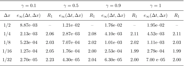
convergence in time we kept ∆x fixed at 10−3 whilst varying ∆t. From the results shown in Tables 1 and 2, by using KBML1 for Eq. (83), it can be seen that, the KBML1 scheme appears to be of orderO(∆x2), andO(∆t1+γ).

Table 1: Numerical accuracy in ∆xapplied to Eq. (83) with ∆t= 10−3 andR1 is order of convergence.

γ= 0.1 γ= 0.5 γ= 0.9 γ= 1

∆x e∞(∆t,∆x) R1 e∞(∆t,∆x) R1 e∞(∆t,∆x) R1 e∞(∆t,∆x) R1

1/2 1.65e–01 – 1.99e–01 – 1.75e–01 – 1.66e–01 –

1/4 3.21e–02 2.36 3.82e–02 2.38 3.17e–02 2.46 2.93e–02 2.50

1/8 7.54e–03 2.09 8.91e–03 2.10 7.26e–03 2.12 6.67e–03 2.13

1/16 1.88e–03 2.01 2.19e–03 2.02 1.78e–03 2.03 1.63e–03 2.03

1/32 4.89e–04 1.94 5.51e–04 1.99 4.43e–04 2.01 4.05e–04 2.01

Table 2: Numerical accuracy in ∆tapplied to Eq. (83) with ∆x= 10−3 andR2 is order of convergence.

γ= 0.1 γ= 0.5 γ= 0.9 γ= 1

∆t e_∞(∆t,∆x) R2 e∞(∆t,∆x) R2 e∞(∆t,∆x) R2 e∞(∆t,∆x) R2

1/10 5.48e–03 – 9.26e–03 – 7.27e–03 – 6.99e–03 –

1/20 2.40e–03 1.19 3.00e–03 1.63 1.87e–03 1.96 1.75e–03 2.00

1/40 1.07e–03 1.16 9.90e–04 1.60 4.83e–04 1.96 4.38e–04 2.00

1/80 4.88e–04 1.14 3.32e–04 1.58 1.25e–04 1.95 1.10e–04 2.00

1/160 2.25e–04 1.12 1.13e–04 1.55 3.30e–05 1.94 2.80e–05 1.98

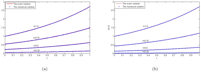
A comparison of the exact and numerical solution of Eq. (83), at the point x = 0.5 and for 0 < t ≤1 for the fractional exponents γ = 0.1, 0.5, and 0.9 with ∆t= 10−3, is shown in Fig. 3. We also show in Fig. 4 the comparison of the exact solution (shown as solid red lines) with the numerical solution (shown as blue dots), at the times t = 0.25, 0.50, 0.75, and 1.00 for γ = 0.1 and 0.9. It can be seen that from both Figs. 3 and 4, for 0 ≤ λq ≤ 1, the approximate solution

Figure 3: (Color online) A comparison of the exact solution (solid red lines) and the numerical solution (blue dots)

for Eq. (83) at the pointx= 0.5 and time 0≤t≤1, forγ= 0.1, 0.5, and 0.9 with ∆t= 10−3_{. Noteγ increases in}

the direction of arrow. (For interpretation of the references to color in this figure legend, the reader is referred to

the web version of this article.)

(a) (b)

Figure 4: (Color online) A comparison of the exact solution (solid red lines) and the numerical solution (blue dots)

for Eq. (83) for (a) γ = 0.1 and (b) γ = 0.9 at the times t = 0.25, 0.50, 0.75, and 1.0 with ∆t = 10−3. (For

interpretation of the references to color in this figure legend, the reader is referred to the web version of this article.)

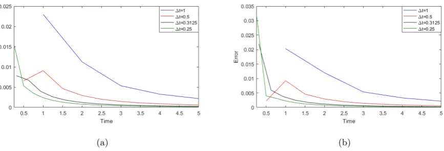
We also investigate the stability in the case 1< λq<2γwhere the analysis was inconclusive. By

calculating the relative error in the numerical solution, we can demonstrate the numerical solution is stable if the error decays with time. In Figs. 5 and 6 we show the relative error for the exponent values γ = 0.6, 0.7, 0.8, and 0.9 at the time t= 5 using increasingly larger time steps ∆t= 0.25, 0.3125, 0.5, and 1. In Fig. 5, for γ = 0.6 and γ = 0.7, we have estimated the ranges of λq as

1.15 ≤λq ≤1.41 and 1.17≤λq ≤1.51 respectively. Likewise in Fig. 6 we have 1.16≤λq ≤1.61

This indicates the solution is stable despite the large time steps chosen.

(a) (b)

Figure 5: (Color online) The relative error for the numerical solution Eq. (83) for (a)γ= 0.6 with 1.15≤λq≤1.41

and (b)γ= 0.7 with 1.17≤λq≤1.51 at timet= 5 and ∆t= 0.25,0.3125,0.5,1.

(a) (b)

Figure 6: (Color online) The relative error for the numerical solution Eq. (83) for (a)γ= 0.8 with 1.16≤λq≤1.61

and (b)γ= 0.9 with 1.14≤λq≤1.73 at the timet= 5 with ∆t= 0.25,0.3125,0.5,1.

Example 6.2. Consider the following fractional Subdiffusion equation with the source term

∂u ∂t =Kγ

∂1−γ ∂t1−γ

∂2u ∂x2

+ (2 +γ)ext1+γ

1−Γ(2 +γ)t γ

Γ(2 + 2γ)

, (86)

with 0< γ≤1 and the initial and fixed boundary conditions

u(x,0) = 0, u(0, t) =t2+γ, u(1, t) =et2+γ. (87)

The exact solution of Eqs. (86) and (87) is

Error and order of convergence estimates for this example is shown in Tables 3 and 4. Similar to the previous example we estimate the convergence in space and time. We see the truncation order of the KBML1 scheme is of order O(∆x2) and O(∆t1+γ).

Table 3: Numerical accuracy in ∆xapplied to Eq. (86) with ∆t= 10−3 andR1 is order of convergence.

γ= 0.1 γ= 0.5 γ= 0.9 γ= 1

∆x e∞(∆t,∆x) R1 e∞(∆t,∆x) R1 e∞(∆t,∆x) R1 e∞(∆t,∆x) R1

1/2 8.87e–03 – 1.21e–02 – 1.76e–02 – 1.95e–02 –

1/4 2.13e–03 2.06 2.87e–03 2.08 4.10e–03 2.11 4.52e–03 2.11

1/8 5.23e–04 2.03 7.07e–04 2.02 1.01e–03 2.02 1.11e–03 2.03

1/16 1.27e–04 2.05 1.76e–04 2.00 2.53e–04 1.99 2.79e–04 1.99

1/32 2.70e–05 2.23 4.30e–05 2.04 6.30e–05 2.00 7.00 e–05 2.00

Table 4: Numerical accuracy in ∆tapplied to Eq. (86) with ∆x= 10−3 andR2 is order of convergence.

γ= 0.1 γ= 0.5 γ= 0.9 γ= 1

∆t e_∞(∆t,∆x) R2 e∞(∆t,∆x) R2 e∞(∆t,∆x) R2 e∞(∆t,∆x) R2

1/10 1.08e–03 – 1.67e–03 – 1.03e–03 – 8.96e–04 –

1/20 4.86e–04 1.16 5.61e–04 1.57 2.69e–04 1.94 2.24e–04 2.00

1/40 2.21e–04 1.14 1.91e–04 1.56 7.00e–05 1.94 5.60e–05 2.00

1/80 1.02e–04 1.12 6.50e–05 1.54 1.80e–05 1.94 1.40e–05 2.01

1/160 4.70e–05 1.11 2.30e–05 1.53 5.00e–06 1.95 3.00e–06 2.02

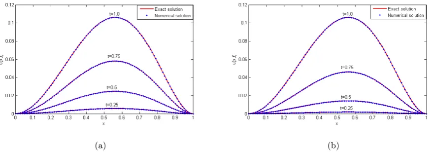
A comparison of the exact and numerical solution of Eq. (86) at the point x= 0.5, 0≤t≤1, forγ = 0.1, 0.5, and 0.9 with ∆t= 10−3, is shown in Fig. 7. In Fig. 8 we also show the comparison of the exact solution (shown as solid red lines) with the numerical solution (shown as blue dots) at the timest = 0.25, 0.5, 0.75, and 1.00, and fractional exponentsγ = 0.1 and 0.9. Again from both Figs. 7 and 8, for 0≤λq≤1, we see the numerical estimates is in agreement with the exact

Figure 7: (Color online) A comparison of the exact solution (solid red lines) and the numerical solution (blue dots)

for Eq. (86) at the pointx= 0.5 and time 0≤t≤1, forγ= 0.1, 0.5, and 0.9 with ∆t= 10−3_{. Noteγ increases in}

the direction of arrow. (For interpretation of the references to color in this figure legend, the reader is referred to

the web version of this article.)

(a) (b)

Figure 8: (Color online) A comparison of the exact solution (solid red lines) and the numerical solution (blue dots)

for Eq. (86) for (a) γ = 0.1 and (b) γ = 0.9 at the times t = 0.25, 0.50, 0.75, and 1.0 with ∆t = 10−3. (For

interpretation of the references to color in this figure legend, the reader is referred to the web version of this article.)

In Figs. 9 and 10 we show again the relative error for the case 1 < λq < 2γ at time t = 5

and ∆t = 1, 0.5, 0.3125, 0.25. The estimated range of λq are 1.15 ≤ λq ≤ 1.41 for γ = 0.6,

1.17 ≤ λq ≤ 1.51 for γ = 0.7, 1.16 ≤ λq ≤ 1.61 for γ = 0.8 and 1.14 ≤ λq ≤ 1.73 for γ = 0.9.

(a) (b)

Figure 9: (Color online) The relative error for the numerical solution Eq. (86), for (a)γ= 0.6 with 1.15≤λq≤1.41

and (b)γ= 0.7 with 1.17≤λq≤1.51 where timet= 5 and ∆t= 0.25,0.3125,0.5,1.

(a) (b)

Figure 10: (Color online) The relative error for the numerical solution Eq. (86), for (a)γ= 0.8 with 1.16≤λq≤1.61

and (b)γ= 0.9 with 1.14≤λq≤1.73 at timet= 5 and ∆t= 0.25,0.3125,0.5,1.

Example 6.3. Consider the following fractional differential equation

∂u ∂t =Kγ

∂1−γ ∂t1−γ

∂2u ∂x2

−αu+f(x, t), (89)

where

f(x, t) =ex

x2(1−x)2

(2 +γ)t1+γ+αt2+γ

−Kγ 2−8x+x2+ 6x3+x4

Γ(3 +γ)t 1+2γ

Γ(2 + 2γ)

,

(90) with 0< γ≤1 and the initial and fixed boundary conditions

The exact solution of Eqs. (89) and (91) is

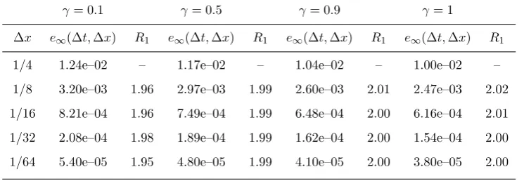
u(x, t) =exx2(1−x)2t2+γ. (92)

The error and order of convergence estimates found from applying the KBML1 scheme on Eq. (89) subject to Eq. (91). Again we estimate the convergence in space and time, the results shown in Tables 5 and 6. It can be seen that the KBML1 scheme appear to be of order O(∆x2) and

O(∆t1+γ_).

Table 5: Numerical accuracy in ∆xapplied to Eq. (89) with ∆t= 10−3 andR1 is order of convergence.

γ= 0.1 γ= 0.5 γ= 0.9 γ= 1

∆x e∞(∆t,∆x) R1 e∞(∆t,∆x) R1 e∞(∆t,∆x) R1 e∞(∆t,∆x) R1

1/4 1.24e–02 – 1.17e–02 – 1.04e–02 – 1.00e–02 –

1/8 3.20e–03 1.96 2.97e–03 1.99 2.60e–03 2.01 2.47e–03 2.02

1/16 8.21e–04 1.96 7.49e–04 1.99 6.48e–04 2.00 6.16e–04 2.01

1/32 2.08e–04 1.98 1.89e–04 1.99 1.62e–04 2.00 1.54e–04 2.00

1/64 5.40e–05 1.95 4.80e–05 1.99 4.10e–05 2.00 3.80e–05 2.00

Table 6: Numerical accuracy in ∆tapplied to Eq. (89) with ∆x= 10−3 _{andR2 is order of convergence.}

γ= 0.1 γ= 0.5 γ= 0.9 γ= 1

∆t e∞(∆t,∆x) R2 e∞(∆t,∆x) R2 e∞(∆t,∆x) R2 e∞(∆t,∆x) R2

1/10 5.85e–04 – 9.71e–04 – 7.78e–04 – 7.54e–04 –

1/20 2.52e–04 1.22 3.13e–04 1.64 2.00e–04 1.96 1.89e–04 2.00

1/40 1.12e–04 1.17 1.03e–04 1.61 5.20e–05 1.96 4.70e–05 2.00

1/80 5.10e–05 1.14 3.40e–05 1.58 1.30e–05 1.95 1.20e–05 1.99

1/160 2.30e–05 1.12 1.20e–05 1.55 4.00e–06 1.92 3.00e–06 1.96

In Fig. 12 we again show the comparison of the exact solution (shown as solid red lines) and the numerical estimate found using the KBML1 methods (shown as blue dots) at the times t= 0.25, 0.5,0.75, and 1.00, with the fractional exponentsγ = 0.1 and 0.9. We also show the comparison of the exact and numerical solution of Eq. (89) at the point x = 0.5, 0≤t ≤1, for γ = 0.1, 0.5, and 0.9 with ∆t= 10−3 in Fig. 11. Again from both Figs. 11 and 12, for 0≤λq ≤1, we see the

Figure 11: (Color online) A comparison of the exact solution (solid red lines) and the numerical solution (blue dots)

for Eq. (89) at the pointx= 0.5 and time 0≤t≤1, forγ= 0.1, 0.5, and 0.9 with ∆t= 10−3_{. Noteγ increases in}

the direction of arrow. (For interpretation of the references to color in this figure legend, the reader is referred to

the web version of this article.)

(a) (b)

Figure 12: (Color online) A comparison of the exact solution (solid red lines) and the numerical solution (blue dots)

for Eq. (89) for (a) γ = 0.1 and (b) γ = 0.9 at the times t = 0.25, 0.50, 0.75, and 1.0 with ∆t = 10−3_{. (For}

interpretation of the references to color in this figure legend, the reader is referred to the web version of this article.)

In this example we also investigate the stability by evaluating the relative error in the numerical predictions in the case 1< λq<2γ. The relative errors are shown in Figs. 13 and 14 for γ = 0.6,

0.7, 0.8 and 0.9 at time t = 5 with ∆t = 0.25, 0.3125, 0.5, 1. The estimated ranges of λq in

these cases are 1.41 ≤λq ≤1.49 for γ = 0.6, 1.48 ≤ λq ≤1.59 for γ = 0.7, 1.55 ≤λq ≤1.71 for γ = 0.8 and 1.61 ≤λq ≤1.83 for γ = 0.9. Again, it can be seen that the relative errors decrease

(a) (b)

Figure 13: (Color online) The relative error for the numerical solution Eq. (89), for (a)γ= 0.6 with 1.41≤λq≤1.49

and (b)γ= 0.7 with 1.48≤λq≤1.59 at the timet= 5 and ∆t= 0.25,0.3125,0.5,1.

(a) (b)

Figure 14: (Color online) The relative error for the numerical solution Eq. (89), for (a)γ= 0.8 with 1.55≤λq≤1.71

and (b)γ= 0.9 with 1.61≤λq≤1.83 at the timet= 5 and ∆t= 0.25,0.3125,0.5,1.

7. Conclusion

In this work, we constructed a Keller Box numerical scheme, KBML1, for the solution of fractional subdiffusion equation. A modification of L1 scheme (ML1) was used to estimate the Riemann–Liouville fractional derivative at the time t_j+1

2. The accuracy of KBML1 was found to

be order 1 +γ in time and second order in space. We proved the stability and convergence of the KBML1 method in the case where 0 < λq <min(_µ1₀,2γ) and 0 < γ ≤ 1. We also demonstrated

the method is also stable numerically in the case where _µ1

0 < λq≤2

γ _{and log}

32≤γ ≤1 by using

for more general equations where we cannot rewrite fractional partial differential equation with a Caputo derivative on the left such as the nonlinear reaction subdiffusion models of Angstmann et al. [41]. This will be a subject of another article in preparation.

Acknowledgments

This work was supported by the Australian Research Council ( ARC DP130100595 ).

Appendix A. Binomial coefficient identity

Using the definition of the binomial coefficient, we can rewrite the coefficient in terms of the Gamma function



 γ

k 

= (−1)k

k k−γ−1

= γΓ(k−γ) Γ(1−γ)

(−1)k−1

k! . (A.1)

[1] H. B. Keller, Numerical Solutions of Partial Differential Equations II, Academic Press, New York, 1971, Ch. A

new difference scheme for parabolic problems, pp. 327–350.

[2] K. B. Oldham, J. Spanier, The Fractional Calculus, Vol. 1047, Academic press New York, 1974.

[3] X. Chen, L. Wei, J. Sui, X. Zhang, L. Zheng, Solving fractional partial differential equations in fluid mechanics by

generalized differential transform method, in: Multimedia Technology (ICMT), 2011 International Conference

on, IEEE, 2011, pp. 2573–2576.

[4] A. A. Elbeleze, A. Kılı¸cman, B. M. Taib, Fractional variational iteration method and its application to fractional

partial differential equation, Math. Probl. Eng. 2013 (2013) Article ID 543848 (10 pages).

[5] W. Schneider, W. Wyss, Fractional diffusion and wave equations, Journal of Mathematical Physics 30 (1) (1989)

134–144.

[6] M. Giona, H. E. Roman, Fractional diffusion equation for transport phenomena in random media, Physica A:

Statistical Mechanics and its Applications 185 (1) (1992) 87–97.

[7] R. Metzler, J. Klafter, The random walk’s guide to anomalous diffusion: a fractional dynamics approach, Physics

reports 339 (1) (2000) 1–77.

[8] B. I. Henry, S. L. Wearne, Fractional reaction–diffusion, Physica A: Statistical Mechanics and its Applications

276 (3) (2000) 448–455.

[9] D. A. Benson, S. W. Wheatcraft, M. M. Meerschaert, Application of a fractional advection-dispersion equation,

Water Resources Research 36 (6) (2000) 1403–1412.

[10] J. H. Cushman, T. R. Ginn, Fractional advection-dispersion equation: a classical mass balance with

convolution-fickian flux, Water resources research 36 (12) (2000) 3763–3766.

[11] A. Atangana, E. Alabaraoye, Solving a system of fractional partial differential equations arising in the model

of HIV infection of CD4+ cells and attractor one-dimensional keller-segel equations, Advances in Difference

[12] P. Roul, Analytical approach for nonlinear partial differential equations of fractional order, Communications in

Theoretical Physics 60 (3) (2013) 269.

[13] V. M´endez, D. Campos, F. Bartumeus, Anomalous diffusion and continuous-time random walks, in: Stochastic

Foundations in Movement Ecology, Springer-Verlag, Berlin, 2014, pp. 113–148.

[14] I. Podlubny, Fractional differential equations, Mathematics in Science and Engineering, Academic Press, New

York and London, 1998.

[15] A. M. Mathai, R. K. Saxena, The H-Function with Applications in Statistics and Other Disciplines, Wiley

Eastern Ltd, New Delhi, 1978.

[16] S. B. Yuste, L. Acedo, An explicit finite difference method and a new von neumann-type stability analysis for

fractional diffusion equations, SIAM J. Numer. Anal. 42 (5) (2005) 1862–1874.

[17] S. Shen, F. Liu, Error analysis of an explicit finite difference approximation for the space fractional diffusion

equation with insulated ends, ANZIAM Journal 46 (2005) 871–887.

[18] F. Liu, P. Zhuang, V. Anh, I. Turner, K. Burrage, Stability and convergence of the difference methods for

the space–time fractional advection–diffusion equation, Applied Mathematics and Computation 191 (1) (2007)

12–20.

[19] Y. Liu, L. Dong, R. Lewis, J.-H. He, Approximate solutions of multi-order fractional advection-dispersion

equation with non-polynomial conditions, International Journal of Numerical Methods for Heat & Fluid Flow

25 (1).

[20] B. Jin, B. Li, Z. Zhou, Discrete maximal regularity of time-stepping schemes for fractional evolution equations,

Numerische Mathematik 138 (1) (2018) 101–131.

[21] W. Deng, M. Chen, E. Barkai, Numerical algorithms for the forward and backward fractional feynman–kac

equations, Journal of Scientific Computing 62 (3) (2015) 718–746.

[22] T. A. M. Langlands, B. I. Henry, The accuracy and stability of an implicit solution method for the fractional

diffusion equation, Journal of Computational Physics 205 (2) (2005) 719–736.

[23] C. M. Chen, F. Liu, K. Burrage, Finite difference methods and a fourier analysis for the fractional reaction–

subdiffusion equation, Applied Mathematics and Computation 198 (2) (2008) 754–769.

[24] D. A. Murio, Implicit finite difference approximation for time fractional diffusion equations, Computers &

Mathematics with Applications 56 (4) (2008) 1138–1145.

[25] H.-l. Liao, Y.-n. Zhang, Y. Zhao, H.-s. Shi, Stability and convergence of modified du fort–frankel schemes for

solving time-fractional subdiffusion equations, Journal of Scientific Computing 61 (3) (2014) 629–648.

[26] W. Yao, J. Sun, B. Wu, S. Shi, Numerical simulation of a class of fractional subdiffusion equations via the

alternating direction implicit method, Numerical Methods for Partial Differential Equations 32 (2) (2016) 531–

547.

[27] C. M. Chen, F. Liu, I. Turner, V. Anh, A fourier method for the fractional diffusion equation describing

sub-diffusion, Journal of Computational Physics 227 (2) (2007) 886–897.

[28] G.-H. Gao, Z.-Z. Sun, H.-W. Zhang, A new fractional numerical differentiation formula to approximate the

Caputo fractional derivative and its applications, Journal of Computational Physics 259 (2014) 33–50.

non-uniform meshes, Journal of Computational Physics 265 (2014) 195–210.

[30] A. A. Alikhanov, A new difference scheme for the time fractional diffusion equation, Journal of Computational

Physics 280 (2015) 424–438.

[31] P. Zhang, H. Pu, A second-order compact difference scheme for the fourth-order fractional sub-diffusion equation,

Numerical Algorithms 76 (2) (2017) 573–598.

[32] R. H. Pletcher, J. C. Tannehill, D. Anderson, Computational fluid mechanics and heat transfer, CRC Press,

2012.

[33] F. S. Al-Shibani, A. I. Ismail, F. A. Abdullah, The Implicit Keller Box method for the one dimensional time

fractional diffusion equation, Journal of Applied Mathematics & Bioinformatics 2 (3).

[34] S. A. Osman, Numerical solution methods for fractional partial differential equations, Ph.D. thesis, University

of Southern Queensland (2017).

[35] F. Zeng, C. Li, A new crank–nicolson finite element method for the time-fractional subdiffusion equation,

Applied Numerical Mathematics 121 (2017) 82–95.

[36] H. B. Keller, A new difference scheme for parabolic problems, in: B. Hubbard (Ed.), Numerical Solutions of

Partial Differential Equations II, Academic Press, New York, 1971, pp. 327–350.

[37] P. Zhuang, F. Liu, V. Anh, I. Turner, New solution and analytical techniques of the implicit numerical method

for the anomalous subdiffusion equation, SIAM Journal on Numerical Analysis 46 (2) (2008) 1079–1095.

[38] C.-M. Chen, F. Liu, V. Anh, I. Turner, Numerical schemes with high spatial accuracy for a variable-order

anomalous subdiffusion equation, SIAM Journal on Scientific Computing 32 (4) (2010) 1740–1760.

[39] M. R. Spiegel, Laplace transforms, McGraw-Hill New York, 1965.

[40] M. R. Spiegel, Advanced mathematics, McGraw-Hill, Incorporated, 1991.

[41] C. N. Angstmann, I. C. Donnelly, B. I. Henry, Continuous time random walks with reactions forcing and