Rochester Institute of Technology
RIT Scholar Works
Theses Thesis/Dissertation Collections
9-2017
Control of Thermal Power System Using Adaptive
Fuzzy Logic Control
Nastaran Naghshineh nxn5534@rit.edu
Follow this and additional works at:https://scholarworks.rit.edu/theses
This Thesis is brought to you for free and open access by the Thesis/Dissertation Collections at RIT Scholar Works. It has been accepted for inclusion in Theses by an authorized administrator of RIT Scholar Works. For more information, please contactritscholarworks@rit.edu.
Recommended Citation
I
______________________________________________________________________________
Control of Thermal Power System Using
Adaptive Fuzzy Logic Control
by
Nastaran Naghshineh
A Thesis Submitted in Partial Fulfilment of the
Requirements for the Degree of Master of Science in Electrical Engineering
Department of Electrical Engineering and Computing Sciences
Rochester Institute of Technology - Dubai
September 2017
II
______________________________________________________________________________ Control of Thermal Power System Using
Adaptive Fuzzy Logic Control
by
Nastaran Naghshineh
A Thesis Submitted in Partial Fulfilment of the Requirements for the Degree of Master of Science in Electrical Engineering Department of Electrical Engineering and Computing Sciences
Approved by:
__________________________________________________________________Date:______________
Dr. Abdulla Ismail
Thesis Advisor – Department of Electrical Engineering and Computing Science
__________________________________________________________________Date:______________
Dr. Ziad El Khatib
Thesis Committee Member – Department of Electrical Engineering and Computing Science
__________________________________________________________________Date:______________
Dr. Rouba Borghol
Thesis Committee Member – Department of Science and Liberal Art
III
Acknowledgements
Firstly, I would like to express my most sincere appreciation to my advisor, Dr. Abdulla Ismail, Professor of Electrical Engineering at Rochester Institute of Technology, for his valuable guidance, consistent encouragement, and continuous support through the completion of this work. Without his endless advices and determined support, this work would have never been possible.
I would like to thank my committee members, Dr. Rouba Borghol, Assistant Professor of Mathematics at Rochester Institute of Technology, and Dr. Ziad El-Khatib, Assistant Professor of Electrical Engineering at Rochester Institute of Technology, for their insights into my thesis.
IV
V
Table of Contents
Abstract ... VII
List of Publications ... VIII
List of Figures ... IX
List of Tables ... XII
List of Symbols ... XIII
List of Abbreviations ... XIV
Chapter 1: Modelling and Simulation of Power System ...1
1.1- Introduction and background knowledge ...1
1.2- Literature review ...3
1.3- Single area modelling and simulation ...5
1.4- Two area modelling and simulation ...8
1.5- Three area modelling and simulation ...13
1.6- N area generalization ...22
Chapter 2: Feedback Modelling and Simulation of Power System Using PID Control ...23
2.1- Introduction to feedback analysis ...23
2.2- Feedback single area modelling and simulation using integral control ...35
2.3- Feedback two area modelling and simulation using integral control...27
2.4- Feedback three area modelling and simulation using integral control...33
2.5- Feedback N area generalization using integral control ...42
Chapter 3: Feedback Modelling and Simulation of Power System Using Adaptive Fuzzy Logic Control ...43
3.1- Introduction to fuzzy logic ...43
3.2- Fuzzy logic control ...44
3.3- Feedback single area modelling and simulation using adaptive fuzzy logic control ...46
3.4- Feedback two area modelling and simulation using adaptive fuzzy logic control ...52
3.5- Feedback three area modelling and simulation using adaptive fuzzy logic control ...58
3.6- Feedback N area generalization using adaptive fuzzy logic control ...66
Chapter 4: Comparison of Conventional PID and Adaptive Fuzzy Logic Control ...68
VI
4.2- Effect of adaptive fuzzy logic control ...68
4.3- Comparison of conventional PID and adaptive fuzzy logic control ...69
Chapter 5: Conclusion and Future Work ...71
5.1- Conclusion ...71
5.2- Conventional vs restructured power system ...71
5.3- Future work ...74
References ...75
Appendix ...77
A - Table of Constants ...77
B - Selected MATLAB file ...78
VII
Abstract
Controlling thermal power systems increases the overall system efficiency and satisfies the desired requirements. In such a large system, fuel reduction of even a small percentage leads to large energy saving. Hence, power systems are gaining significant attention from engineers and scientists.
In this thesis, the uncontrolled power system for single area, two area, and three area is modelled using state space representation. Frequency deviation is simulated using MATLAB and SIMULINK. PID control is added to the system to analyze the effect of conventional control on system output response. Adaptive fuzzy logic control is added to the uncontrolled system using MATLAB Fuzzy Inference System and its effect on the system output response is measured in terms of overshoot/undershoot percentage, settling time, and steady state frequency error. Effect of adaptive fuzzy logic control is analyzed on single area, two area, and three area power system. Tie-line power exchange among areas is investigated before and after implementation of PID and adaptive fuzzy logic control.
VIII
List of Publications
[1] Nastaran Naghshineh, Dr. Abdulla Ismail. Comprehensive Approach Towards Modelling and Simulation of Single Area Power Generation System using PI Control and Stability Solution using Linear Quadratic Regulator. International Research Journal of Engineering and Technology (IRJET). August 2017.
[2] Nastaran Naghshineh, Dr. Abdulla Ismail. Advanced Optimization of Single Area Power Generations System using Adaptive Fuzzy Logic and PI Control. International Research Journal of Engineering and Technology (IRJET). August 2017.
IX
List of Figures
Figure 1.1: Block diagram of power system
Figure 1.2: Two main control loops of Automatic Generation Control
Figure 1.3: Block diagram of single area LFC system
Figure 1.4: Block diagram of single area LFC system with state variable assignment
Figure 1.5: Output response of single area LFC system
Figure 1.6: Two area interconnected power system
Figure 1.7: Block diagram of two area LFC system
Figure 1.8: Output response of area 1 in two area LFC system
Figure 1.9: Output response of area 2 in two area LFC system
Figure 1.10: Tie-line response of two area LFC system
Figure 1.11: Three area interconnected power system
Figure 1.12: Block diagram of three area LFC system
Figure 1.13: Output response of area 1 in three area LFC system
Figure 1.14: Output response of area 2 in three area LFC system
Figure 1.15: Output response of area 3 in three area LFC system
Figure 1.16: Tie-line response of three area LFC system for area 1 and 2
Figure 1.17: Tie-line response of three area LFC system for area 2 and 3
Figure 1.18: Four area interconnected power system
Figure 2.1: Implementation of PID control in feedback system
Figure 2.2: Block diagram of feedback single area LFC system
Figure 2.3: Output response of feedback single area LFC system with PI control
Figure 2.4: Block diagram of feedback two area LFC system with integral control
Figure 2.5: Output response of area 1 in feedback two area LFC system with integral control
X
Figure 2.7: Tie-line response of two area LFC system with integral control
Figure 2.8: Block diagram of feedback three area LFC system with integral control
Figure 2.9: Output response of area 1 in feedback three area LFC system with integral control
Figure 2.10: Output response of area 2 in feedback three area LFC system with integral control
Figure 2.11: Output response of area 3 in feedback three area LFC system with integral control
Figure 2.12: Tie-line response of feedback three area LFC system with integral control for area 1 and 2
Figure 2.13: Tie-line response of feedback three area LFC system with integral control for area 2 and 3
Figure 2.14: Tie-line response of feedback three area LFC system with integral control for area 1 and 3
Figure 3.1: Fuzzy logic control block diagram
Figure 3.2: FIS - inputs and output
Figure 3.3: FIS - membership functions
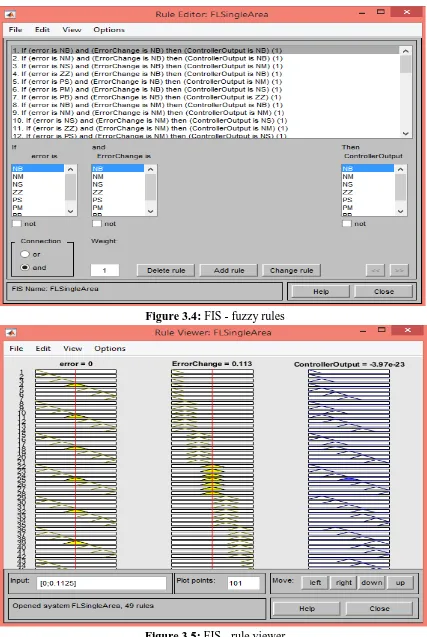
Figure 3.4: FIS - fuzzy rules
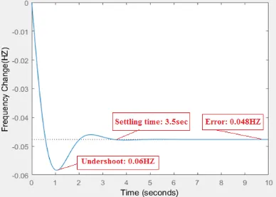
Figure 3.5: FIS - rule viewer
Figure 3.6: Block diagram of open loop single area LFC system
Figure 3.7: Output response of open loop single area LFC system
Figure 3.8: Block diagram of feedback single area LFC system with adaptive FL and PI control
Figure 3.9: Output response of feedback single area LFC system with adaptive FL and PI control
Figure 3.10: Block diagram of open loop two area LFC system
Figure 3.11: Output response of area 1 in open loop two area LFC system
Figure 3.12: Output response of area 2 in open loop two area LFC system
Figure 3.13: Tie-line response of open loop two area LFC system
XI
Figure 3.15: Output response of area 1 in feedback two area LFC system with adaptive FL and PI control
Figure 3.16: Output response of area 2 in feedback two area LFC system with adaptive FL and PI control
Figure 3.17: Tie-line response of feedback two area LFC system with adaptive FL and PI control
Figure 3.18: Block diagram of open loop three area LFC system
Figure 3.19: Output response of area 1 in open loop three area LFC system
Figure 3.20: Output response of area 2 in open loop three area LFC system
Figure 3.21: Output response of area 3 in open loop three area LFC system
Figure 3.22: Tie-line response of open loop three area LFC system for area 1 and 2
Figure 3.23: Tie-line response of open loop three area LFC system for area 2 and 3
Figure 3.24: Block diagram of feedback three area LFC system with adaptive FL and PI control
Figure 3.25: Output response of area 1 in three area LFC system with adaptive FL and PI control
Figure 3.26: Output response of area 2 in three area LFC system with adaptive FL and PI control
Figure 3.27: Output response of area 3 in three area LFC system with adaptive FL and PI control
Figure 3.28: Tie-line response of feedback three area LFC system for area 1 and 2
Figure 3.29: Tie-line response of feedback three area LFC system for area 2 and 3
Figure 3.30: Tie-line response of feedback three area LFC system for area 1 and 3
Figure 3.31: Five area interconnected power system
Figure 3.32: Six area interconnected power system
Figure 4.1: Fuzzy logic system
Figure 4.2: Vertically integrated structure
Figure 4.3: Restructured/ deregulated environment
XII
List of Tables
Table 2.1: Control parameters for feedback single LFC system
Table 2.2: Control parameters for feedback two area LFC system
Table 2.3: Control parameters for feedback three area LFC system
Table 3.1: Fuzzy rules for LFC system
Table 3.2: Control parameters for feedback single area LFC system with adaptive FL control
Table 3.3: Control parameters for feedback two area LFC system with adaptive FL control
Table 3.4: Control parameters for feedback three area LFC system with adaptive FL control
Table 3.5: Relationship between number of control areas and number of outputs
XIII
List of Symbols
Symbol
Description
𝑇𝑇𝑔𝑔 Governor Time Constant
𝑇𝑇𝑡𝑡 Turbine Time Constant
𝑇𝑇𝑟𝑟 Re-heat Time Constant
𝑇𝑇𝑝𝑝 Generator Time Constant
𝑇𝑇1 Governor Time Constant of Area 2 – Block 1
𝑇𝑇2 Governor Time Constant of Area 2 – Block 2
𝑇𝑇3 Governor Time Constant of Area 2 – Block 3
𝑇𝑇4 Turbine Time Constant of Area 2 – Block 1
𝑇𝑇5 Turbine Time Constant of Area 2 – Block 2
𝑇𝑇6 Re-heat Time Constant of Area 2
𝑇𝑇7 Feedforward Time Constant of Area 2
𝑇𝑇8 Generator Time Constant of Area 2
𝑇𝑇𝑣𝑣1 Governor Time Constant of Area 2
𝑇𝑇𝑣𝑣2 Governor Time Constant of Area 2
T Tie-Line Time Constant
𝐾𝐾𝑟𝑟 Re-heat Gain Coefficient
𝐾𝐾𝑃𝑃 Generator Gain Coefficient
𝑅𝑅𝑖𝑖 Speed Regulation or Droop of Area i
𝐾𝐾1 Governor Gain Coefficient of Area 2 – Block 1
𝐾𝐾2 Turbine Gain Coefficient of Area 2 – Block 2
𝐾𝐾3 Re-heat Gain Coefficient of Area 2
𝐾𝐾4 Feedforward Gain Coefficient of Area 2
𝐾𝐾5 Generator Gain Coefficient of Area 2
Δ𝑃𝑃𝑐𝑐 Speed Changer Amount
Δ𝑃𝑃𝑑𝑑 Change in Load (Disturbance)
Δf System Frequency Change
𝑃𝑃𝑡𝑡𝑖𝑖𝑡𝑡,12 Tie-Line Power Exchange From Area 1 to Area 2
𝑃𝑃𝑡𝑡𝑖𝑖𝑡𝑡,21 Tie-Line Power Exchange From Area 2 to Area 1
𝑃𝑃𝑡𝑡𝑖𝑖𝑡𝑡,23 Tie-Line Power Exchange From Area 2 to Area 3
𝑃𝑃𝑡𝑡𝑖𝑖𝑡𝑡,32 Tie-Line Power Exchange From Area 3 to Area 2
𝑃𝑃𝑡𝑡𝑖𝑖𝑡𝑡,13 Tie-Line Power Exchange From Area 1 to Area 3
𝑃𝑃𝑡𝑡𝑖𝑖𝑡𝑡,31 Tie-Line Power Exchange From Area 3 to Area 1
𝑋𝑋𝑖𝑖 ith State Variable
𝐾𝐾𝑔𝑔 Proportional Gain Constant
𝐾𝐾𝑖𝑖 Integral Gain Constant
𝐾𝐾𝑑𝑑 Derivative Gain Constant
𝐵𝐵𝑛𝑛 Frequency Bias Factor
e(t) System Error
u(t) Plant Input
XIV
List of Abbreviations
Abbreviation
Description
AGC Automatic Generation Control
LFC Load Frequency Control
AVR Automatic Voltage Regulator
IC Integral Control
FL Fuzzy Logic
ACE Area Control Error
PI Proportional and Integral
PD Proportional and Derivative
PID Proportional, Integral and Derivative
LQR Linear Quadratic Regulator
NB Negative Big
NM Negative Medium
NS Negative Small
ZZ Zero
PS Positive Small
PM Positive Medium
PB Positive Big
Genco Generation Company
1
Chapter 1: Modelling and Simulation of Power System
1.1
Introduction and background knowledge
The aim in control of thermal power system “is to make the generator’s fuel consumption or the operating cost of the whole system minimal by determining the power output of each generating unit under the constraint condition of the system load demands.”[3] Configuration of a power plant is to select the optimal operation conditions in order to satisfy the electricity demand while maximizing the net income and minimizing the total operation cost [5].
Electric loads are energy consumptions which range from household appliances to industrial machinery. In Electric power generation system, the load variation changes continuously and the objective is to ensure the generation variations match the load variations at the minimal conditions or cost. In other words, the large interconnected power system must maintain the voltage and the frequency variations within a very narrow range. When the system experiences disturbances from load changes, the generator controllers must act quickly to maintain the balance and dampen the oscillations experienced by the system [4]. Control of electric energy system in order to obtain exact matching between the generation and the load is a very complex task as load varies every hour or even every minute.
2
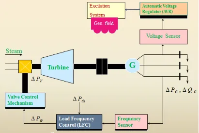
[image:17.612.109.520.73.347.2]Figure 1.1: Block diagram of power system
3
Figure 1.3 shows the block diagram representation of single area LFC system which consists of a speed governor, a turbine, a re-heater, and a generator [19]. In some LFC systems, no re-heat component is available. Re-heat or feed water re-heat is used to pre-heat the water that is delivered to the steam boiler. In this thesis, all the considered models have re-heat component. For computational simplicity in LFC problem, we consider the case where the thermal power generation system consists of a single boiler, a single turbine, and a single generator. In many real world power systems, the generation unit consists of multiple boilers, steam turbines, and generators. “Network Power Loss” is referred to the loss of power from one generator to another or from one turbine to another that is experienced in systems with multiple components of same type [3].
In Figure 1.3, the inputs of the system are Δ𝑃𝑃𝑐𝑐 representing the change in speed governor by utility and Δ𝑃𝑃𝑑𝑑 representing the change in load by consumer also known as disturbance. The output of LFC system is Δf which represents the change or variation in system frequency. The objective is to have a constant output frequency which corresponds to Δf being zero or very small. The value of speed regulation R also known as droop is the ratio of frequency deviation (Δf) to change in power output of the generator.
Figure 1.3: Block diagram of single area LFC system
1.2
Literature review
4
Performance of the uncontrolled system shown in Figure 1.3 is undesirable in terms of settling time, steady state error, and initial transient response. Proportional and Integral (PI), Proportional and Derivative (PD), or Proportional, Integral and Derivative (PID) control can be used to secure the system performance when changes occur on the power system parameters. There exist two stabilization techniques: Pole-Placement technique and Linear Quadratic Regulator (LQR) [6]. In this thesis, LQR technique is used to stabilize the system once a control is added. PID control is a powerful and well known tool to improve both transient and steady state performances. However, proper tuning of PID control can be a very complex task as there are three parameters (𝐾𝐾𝑔𝑔,𝐾𝐾𝑖𝑖,𝐾𝐾𝑑𝑑) to be properly tuned to give the desired output response [7]. In [7], instructions of PID control tuning using MATLAB are explained in details. In [6], steady state performance of a two area interconnected thermal power system is considered after implementation of PI control.
Conventional PI control is very successful in achieving zero steady state error in power system. However, the load is continuously changing. Hence, conventional PI control will no longer be suitable to solve the control problem due to dynamic nature of the system [8]. Additionally, PI control approach returns relatively undesirable dynamic performance as evident by large overshoot/undershoot and transient frequency oscillation. Furthermore, settling time achieved by PI control is relatively large [14].
The problem of controlling and optimizing a dynamic system can be addressed using Fuzzy Logic. In various applications, Fuzzy Logic (FL) has been used to solve power plant control problem because it is well suited for uncertain systems. FL has been applied to solve optimal distribution planning, generator maintenance scheduling, load forecasting, load management, and generation dispatch problem [4]. FL establishes linguistic rules, called membership rules, to determine a systematic way of describing controller actions. Reliability of FL control makes it applicable in solving wide range of control problems such as power system control.
5
Simulation results show that the system performance is significantly improved in terms of settling time, steady state frequency deviation, and percentage undershoot.
1.3 Single area modelling and simulation
Open loop modelling and simulation begins with considering a single area LFC system. As shown in Figure 1.4, the output of each integrator is a state space variable. Equations 1.1-1.4 show the transfer functions developed using the state assignments shown in Figure 1.4.
Block 1: Generator 𝑋𝑋1 𝑋𝑋2−Δ𝑃𝑃𝑑𝑑 =
𝐾𝐾𝑝𝑝
1+𝑇𝑇𝑝𝑝𝑆𝑆 (1.1)
Block 2: Re-heat 𝑋𝑋2 𝑋𝑋3 =
1+𝐾𝐾𝑟𝑟𝑆𝑆
1+𝑇𝑇𝑟𝑟𝑆𝑆 (1.2)
Block 3: Turbine 𝑋𝑋3 𝑋𝑋4 =
1
1+𝑇𝑇𝑡𝑡𝑆𝑆 (1.3)
Block 4: Governor −1 𝑋𝑋4
𝑅𝑅 𝑋𝑋1+Δ𝑃𝑃𝑐𝑐
= 1
1+𝑇𝑇𝑔𝑔𝑆𝑆 (1.4)
Figure 1.4: Block diagram of single area LFC system with state variable assignment
The above system has two inputs: ΔPc and ΔPd. The output of the system is Δ𝑓𝑓 which represents change or variation in system frequency. To develop state space representation of the system shown in Figure 1.4, rate of change of each state variable is needed. Equations 1.5-1.8 are the system state equations:
Block 1: Generator 𝑥𝑥1̇ = −1 𝑇𝑇𝑝𝑝 𝑥𝑥1 +
𝐾𝐾𝑝𝑝
𝑇𝑇𝑝𝑝 𝑥𝑥2 -
𝐾𝐾𝑝𝑝
𝑇𝑇𝑝𝑝 Δ𝑃𝑃𝑑𝑑 (1.5)
Block 2: Re-heat 𝑥𝑥2̇ = −1 𝑇𝑇𝑟𝑟 𝑥𝑥2 +
1 𝑇𝑇𝑟𝑟 (1−
𝐾𝐾𝑟𝑟
𝑇𝑇𝑡𝑡)𝑥𝑥3 +
𝐾𝐾𝑟𝑟
6
Block 3: Turbine 𝑥𝑥3̇ = −1 𝑇𝑇𝑡𝑡 𝑥𝑥3 +
1
𝑇𝑇𝑡𝑡𝑥𝑥4 (1.7)
Block 4: Governor 𝑥𝑥4̇ = −1 𝑅𝑅𝑇𝑇𝑔𝑔 𝑥𝑥1 -
1 𝑇𝑇𝑔𝑔 𝑥𝑥4 +
1
𝑇𝑇𝑔𝑔Δ𝑃𝑃𝑐𝑐 (1.8)
Then, Equations 1.5-1.8 are transformed into state space model. It is important to note that the output of the system Δ𝑓𝑓 is the state variable𝑥𝑥1. State space representation of the single area LFC system shown in Figure 1.4 is:
𝑿𝑿̇(𝒕𝒕)=A X(t) + B Δ𝑷𝑷𝒄𝒄 + F Δ𝑷𝑷𝒅𝒅 (1.9)
Y(t)= C X(t) (1.10)
• • • • 4 3 2 1 x x x x = − − − − − − g g t t r t r r t r r p p p T RT T T T T K T T K T T K T 1 0 0 1 1 1 0 0 1 1 1 0 0 0 1 4 3 2 1 x x x x + g T 1 0 0 0
Δ𝑃𝑃𝑐𝑐 +
− 0 0 0 p p T K
Δ𝑃𝑃𝑑𝑑
Δf =
[
1 0 0 0]
4 3 2 1 x x x x7
B =
−
0 0 0 p p
T K
The corresponding parameters for the state, input, and output matrix are given in the Appendix A-1. The input ΔPd is a unit step function. Figure 1.5 illustrates the output response of the LFC system. Increase in load leads to decrease in frequency which corresponds to undershoot. Decrease in load leads to increase in frequency which corresponds to overshoot. The system settling time is about 180 seconds and the frequency deviation is -2.5HZ. The undershoot percentage, settling time, and the steady state error are significantly large and this leads to the necessity of having PID control added to the system.
8
1.4
Two area modelling and simulation
The main reasons for utilities to interconnect control areas are:
1. To buy or sell power with neighboring control areas whose operation cost are different from theirs.
2. To improve reliability of control areas for events such as sudden loss in generation.
Total generation is divided among the control areas adequately such that the production cost is minimized. This means each control area must participate in generating electricity and regulating frequency. When power interchange scheduling among the areas is on, each control area is responsible to generate the scheduled amount of electricity and interchange some electricity with other control areas. This interchange will allow the neighboring control areas to generate sufficient amount of electricity when load changes.
In a two area interconnected power system there is tie-line power exchange flowing from area 1 to area 2, called 𝑃𝑃𝑡𝑡𝑖𝑖𝑡𝑡,12 . The tie-line power exchange running from area 2 to area 1 is the same as that of area 1 to area 2 in magnitude but opposite in direction. Figure 1.6 illustrates the concept of two area power system with tie-line power.
𝑃𝑃𝑡𝑡𝑖𝑖𝑡𝑡,21
𝑃𝑃𝑡𝑡𝑖𝑖𝑡𝑡,12
𝑃𝑃𝑡𝑡𝑖𝑖𝑡𝑡,12= - 𝑃𝑃𝑡𝑡𝑖𝑖𝑡𝑡,21
Figure 1.6: Two area interconnected power system
Figure 1.7 shows the block diagram representation of a two area interconnected LFC system. Area 1 and area 2 can have the same model; however, in Figure 1.7, two different areas are combined together to show a two area power system. Area 1 consists of 4 transfer function blocks and area 2 consists of 8 transfer function blocks. 𝛥𝛥𝑃𝑃𝑡𝑡𝑖𝑖𝑡𝑡,12 is output of tie-line power integral block which interconnects the two area. 𝛥𝛥𝑃𝑃𝑡𝑡𝑖𝑖𝑡𝑡,12 represents the incremental power change in tie-line. Hence, the entire system is modelled by 13 state variables.
9
Figure 1.7: Block diagram of two area LFC system
10 − − − − − − − − − − − 7 1 1 2 2 2 1 1 3 2 1 2 1 3 3 4 4 5 2 5 6 3 6 8 5 8 5 1 0 0 0 0 0 0 0 1 0 0 0 0 0 0 ) 1 ( 1 1 0 0 0 0 0 ) 1 ( ) 1 ( 1 1 0 0 0 0 0 0 1 1 0 0 0 0 0 0 1 0 0 0 0 0 0 1 0 0 0 0 0 0 0 0 0 0 0 0 0 0 0 0 0 0 0 0 0 0 0 0 0 0 0 0 0 0 0 0 0 0 0 0 0 0 0 0 T T T T T T T T T T T T T T T T T T K T T K T T K T K v v v v
The inputs of the system are Δ𝑃𝑃𝑑𝑑1 and Δ𝑃𝑃𝑑𝑑2, respectively. Following is the input matrix of the system:
11
The system has three outputs. The first output is frequency deviation of area 1 (Δ𝑓𝑓1 =
𝑥𝑥1), the second output is frequency deviation of area 2 (Δ𝑓𝑓2 = 𝑥𝑥6), and the third output is tie-line power connecting area 1 and 2 which is represented by state variable𝑥𝑥5. Following is the output matrix of the system:
C=
0 0 0 0 0 0 0 0 1 0 0 0 0
0 0 0 0 0 0 0 1 0 0 0 0 0
0 0 0 0 0 0 0 0 0 0 0 0 1
Figures 1.8 and 1.9 show the output response of area 1 and area 2, respectively. Similar to the single area system, in two area system the objective is to have a system with zero steady state frequency deviation Δ𝑓𝑓1= Δ𝑓𝑓2= 0. By examining the responses, it can be clearly seen that the system is behaving undesirably. Output responses of area 1 and 2 take about 300 seconds to reach a steady value. This is an extremely slow settling time with about 40% frequency error. The undesirable system performance determines the necessity of integral control in the system. Integral control can significantly reduce steady state error, improve settling time, and decrease undershoot. Integral control ensures Area Control Error (ACE) is reduced to zero or nearly zero at steady state. ACE is the difference between the actual power flow out of area, and scheduled power flow.
12
Figure 1.8: Output response of area 1 in two area LFC system
13
Figure 1.10: Tie-line response of two area LFC system
1.5
Three Area Modelling and Simulation
14
𝑃𝑃𝑡𝑡𝑖𝑖𝑡𝑡,12 = - 𝑃𝑃𝑡𝑡𝑖𝑖𝑡𝑡,21 𝑃𝑃𝑡𝑡𝑖𝑖𝑡𝑡,13 = - 𝑃𝑃𝑡𝑡𝑖𝑖𝑡𝑡,31 𝑃𝑃𝑡𝑡𝑖𝑖𝑡𝑡,23 = - 𝑃𝑃𝑡𝑡𝑖𝑖𝑡𝑡,32
Figure 1.11: Three area interconnected power system
Figure 1.12 shows the block diagram of three area interconnected system. Three area system is extension of two area system with an additional control area. In Figure 1.12, area 1 and 3 are identical. Each area has a reference input as well as disturbance. Considering the disturbances or load changes to be the only inputs of the LFC system, the entire system has 3 inputs: Δ𝑃𝑃𝑑𝑑1, Δ𝑃𝑃𝑑𝑑2, and Δ𝑃𝑃𝑑𝑑3.
Output of area 1 is Δ𝑓𝑓1 and the state variable 𝑥𝑥1 is used to represent the corresponding output response. Output of area 2 is Δ𝑓𝑓2 and the state variable 𝑥𝑥6 is used to represent the corresponding output response. Output of area 3 is Δ𝑓𝑓3 and the state variable 𝑥𝑥15 is used to represent the corresponding output response.
15
variable 𝑥𝑥14. Lastly, there is an integral block connecting area 1 and 3. The corresponding output of this block is 𝑃𝑃𝑡𝑡𝑖𝑖𝑡𝑡,13which is the state variable𝑥𝑥19.
Figure 1.12: Block diagram of three area LFC system
Equations 1.11-1.32 are the transfer functions of each block used in Figure 1.12. The parameters are given in the Appendix A-1.
Block 1: Generator 1 𝐾𝐾𝑝𝑝
1+𝑇𝑇𝑝𝑝𝑆𝑆 (1.11)
Block 2: Re-Heat 1 1+𝐾𝐾𝑟𝑟𝑆𝑆
1+𝑇𝑇𝑟𝑟𝑆𝑆 (1.12)
Block 3: Turbine 1 1
16
Block 4: Governor 1 1
1+𝑇𝑇𝑔𝑔𝑆𝑆 (1.14)
Block 5: Tie-Line 1 and 2 2𝜋𝜋𝑇𝑇
𝑆𝑆 (1.15)
Block 6: Generator 2 𝐾𝐾5
1+𝑇𝑇8𝑆𝑆 (1.16)
Block 7: Re-Heat 2 𝐾𝐾3
1+𝑇𝑇6𝑆𝑆 (1.17)
Block 8: Turbine Part 2 𝐾𝐾2
1+𝑇𝑇5𝑆𝑆 (1.18)
Block 9: Turbine Part 1 1
1+𝑇𝑇4𝑆𝑆 (1.19)
Block 10: Governor Part 3 1+𝑇𝑇𝑣𝑣1𝑆𝑆
1+𝑇𝑇3𝑆𝑆 (1.20)
Block 11: Governor Part 2 1+𝑇𝑇𝑣𝑣2𝑆𝑆
1+𝑇𝑇2𝑆𝑆 (1.21)
Block 12: Governor Part 1 𝐾𝐾1
1+𝑇𝑇1𝑆𝑆 (1.22)
Block 13: Feedforward 𝐾𝐾4
1+𝑇𝑇7𝑆𝑆 (1.23)
Block 14: Tie-Line 2 and 3 2𝜋𝜋𝑇𝑇
𝑆𝑆 (1.24)
Block 15: Generator 3 𝐾𝐾𝑝𝑝
1+𝑇𝑇𝑝𝑝𝑆𝑆 (1.25)
Block 16: Re-Heat 3 1+𝐾𝐾𝑟𝑟𝑆𝑆
1+𝑇𝑇𝑟𝑟𝑆𝑆 (1.26)
Block 17: Turbine 3 1
1+𝑇𝑇𝑡𝑡𝑆𝑆 (1.27)
Block 18: Governor 3 1
1+𝑇𝑇𝑔𝑔𝑆𝑆 (1.28)
Block 19: Tie-Line 1 and 3 2𝜋𝜋𝑇𝑇
𝑆𝑆 (1.29)
Droop 1 1
17
Droop 2 1
𝑅𝑅2 (1.31)
Droop 3 1
𝑅𝑅3 (1.32) As illustrated in Figure 1.12, area 1, 2, and 3 consist of 4, 8, and 4 transfer function blocks, respectively. There are 3 integral blocks to connect the areas. Hence, there are 19 state variables in Figure 1.12. The system has 3 inputs: Δ𝑃𝑃𝑑𝑑1, Δ𝑃𝑃𝑑𝑑2, and Δ𝑃𝑃𝑑𝑑3. The system has 6 outputs: Δ𝑓𝑓1, Δ𝑓𝑓2, Δ𝑓𝑓3, Δ𝑃𝑃𝑡𝑡𝑖𝑖𝑡𝑡,12,Δ𝑃𝑃𝑡𝑡𝑖𝑖𝑡𝑡,23, and Δ𝑃𝑃𝑡𝑡𝑖𝑖𝑡𝑡,31.
19 − − − = 0 0 0 0 0 0 0 0 0 0 0 0 0 0 0 0 0 0 0 0 0 0 0 0 0 0 0 0 0 0 0 0 0 0 0 0 0 0 0 0 0 0 0 0 0 0 0 0 0 0 0 0 0 0 8 5 p p P P T K T K T K B = 1 0 0 0 0 0 0 0 0 0 0 0 0 0 0 0 0 0 0 0 0 0 0 0 1 0 0 0 0 0 0 0 0 0 0 0 0 0 0 0 0 0 0 0 0 0 0 0 0 0 0 0 1 0 0 0 0 0 0 0 0 1 0 0 0 0 0 0 0 0 0 0 0 0 0 0 0 0 0 0 0 0 0 0 0 0 0 0 0 1 0 0 0 0 0 0 0 0 0 0 0 0 0 0 0 0 0 0 0 0 0 0 0 1 C
20
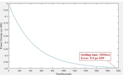
Figures 1.16 and 1.17 show the tie-line power exchange. The tie-line power exchange begins at zero and experiences undershoot due to presence of disturbance. The response settles after 25 seconds at -0.5pu MW. The objective is to eliminate or minimize the steady state power exchange deviation.
Figure 1.13: Output response of area 1 in three area LFC system
21
Figure 1.15: Output response of area 3 in three area LFC system
22
Figure 1.17: Tie-line response of three area LFC system for area 2 and 3
1.6
N area generalization
The single area, two area, and three area systems considered in the previous sections are test cases. By analyzing the output responses of the test cases, it is concluded that the uncontrolled LFC system of size N will have unsatisfactory performance in terms of percentage overshoot/undershoot, oscillations, settling time, and steady state error. The need for control is essential in regulating the output response and improving overall performance of the system.
23
Figure 1.18: Four area interconnected power system
Chapter 2: Feedback Modelling and Simulation of Power
System Using PID Control
2.1 Introduction to feedback analysis
The primary objective of using control in power system is to eliminate or minimize the system frequency deviation. In typical power systems, following performance specifications are recommended:
1. Steady state error should not be more than 0.01HZ. 2. Settling time should be less than 3 seconds.
3. The maximum overshot/undershoot should not be more than 6% which corresponds to 0.06HZ.
4. Change in power exchange Δ𝑃𝑃𝑡𝑡𝑖𝑖𝑡𝑡is upon mutual agreement of the generating areas.
Each type of control has different role in a system. Proportional control is used to reduce rise time and settling time. Integral control is used to eliminate steady state error. The negative effect of integral control is creating oscillation. Derivative control is used to improve transient
AREA 1
AREA 2
AREA 3
AREA 4
Δ𝑓𝑓2
Δ𝑓𝑓4
Δ𝑓𝑓1
Δ𝑓𝑓3
Δ𝑃𝑃𝑡𝑡𝑖𝑖𝑡𝑡,34
Δ𝑃𝑃𝑡𝑡𝑖𝑖𝑡𝑡,21
Δ𝑃𝑃𝑡𝑡𝑖𝑖𝑡𝑡,24
Δ𝑃𝑃𝑡𝑡𝑖𝑖𝑡𝑡,31
Δ𝑃𝑃𝑡𝑡𝑖𝑖𝑡𝑡,23
24
response which means reducing overshoot/undershoot. Equations 2.1-2.5 show structure of most commonly used conventional controls:
Proportional (P) control: U(S) = 𝐾𝐾𝑔𝑔 E(S) (2.1)
Integral (I) control: U(S) = 𝐾𝐾𝑖𝑖
𝑆𝑆 E(S) (2.2)
Derivative (D) Control: U(S) = (𝐾𝐾𝑑𝑑S) E(S) (2.3)
PI control: U(S) = (𝐾𝐾𝑔𝑔+ 𝐾𝐾𝑖𝑖
𝑆𝑆) E(S) (2.4)
PID control: U(S) = (𝐾𝐾𝑔𝑔+ 𝐾𝐾𝑖𝑖
𝑆𝑆 + 𝐾𝐾𝑑𝑑S) E(S) (2.5)
The main objective in LFC system control problem is to improve the dynamic response of the system by minimizing or even eliminating AEC. In real life LFC systems, ACE is never zero due to instantaneous change in load. Hence, the objective is to keep AEC as close to zero as possible. Integral control is well suited in this case to meet the objective. The value of integral gain constant 𝐾𝐾𝑖𝑖 is adjusted until the desired response is achieved. This is called tuning and is a time consuming task [6]. Figure 2.1 illustrates how a conventional PID control can be added to a system. “Process” block in Figure 2.1 is the uncontrolled system. When an integral control is added to a system, a new pole is added to the system which may cause the system to be unstable. This means a stabilizing technique is needed. LQR technique is used to stabilize the system.
25
2.2 Feedback single area modelling and simulation using PI
control
For a single area closed loop system, a PI control is added in the block diagram as shown in Figure 2.2. The transfer function of the PI control is (𝐾𝐾𝑔𝑔 + 𝐾𝐾𝑖𝑖
𝑆𝑆).
Figure 2.2: Block diagram of feedback single area LFC system
The system shown in Figure 2.2 has 5 transfer function blocks which corresponds to 5 state variables. Equations 2.6-2.10 show the developed transfer functions of Figure 2.2.
Block 1: Generator 𝑋𝑋1 𝑋𝑋2−Δ𝑃𝑃𝑑𝑑 =
𝐾𝐾𝑝𝑝
1+𝑇𝑇𝑝𝑝𝑆𝑆 (2.6)
Block 2: Re-Heat 𝑋𝑋2 𝑋𝑋3 =
1+𝐾𝐾𝑟𝑟𝑆𝑆
1+𝑇𝑇𝑟𝑟𝑆𝑆 (2.7)
Block 3: Turbine 𝑋𝑋3 𝑋𝑋4 =
1
1+𝑇𝑇𝑡𝑡𝑆𝑆 (2.8)
Block 4: Governor −1 𝑋𝑋4
𝑅𝑅 𝑋𝑋1+Δ𝑃𝑃𝑐𝑐
= 1
1+𝑇𝑇𝑔𝑔𝑆𝑆 (2.9)
Block 5: PI Control 𝑋𝑋5 𝑋𝑋1 =
𝐾𝐾𝑔𝑔𝑆𝑆+𝐾𝐾𝑖𝑖
𝑆𝑆 (2.10)
Equations 2.11-2.15 show the system differential equations which corresponds to rate of change of each variable:
𝑥𝑥1̇ = −1 𝑇𝑇𝑝𝑝 𝑥𝑥1 +
𝐾𝐾𝑝𝑝
𝑇𝑇𝑝𝑝 𝑥𝑥2 -
𝐾𝐾𝑝𝑝
𝑇𝑇𝑝𝑝 Δ𝑃𝑃𝑑𝑑 (2.11)
𝑥𝑥2̇ = −1 𝑇𝑇𝑟𝑟 𝑥𝑥2 +
1 𝑇𝑇𝑟𝑟 (1−
𝐾𝐾𝑟𝑟
𝑇𝑇𝑡𝑡)𝑥𝑥3 +
𝐾𝐾𝑟𝑟
26
𝑥𝑥3̇ = −1 𝑇𝑇𝑡𝑡 𝑥𝑥3 +
1
𝑇𝑇𝑡𝑡𝑥𝑥4 (2.13)
𝑥𝑥4̇ = 𝑅𝑅𝑇𝑇−1𝑔𝑔𝑥𝑥1 - 𝑇𝑇1𝑔𝑔𝑥𝑥4 - 𝑇𝑇1𝑔𝑔𝑥𝑥5 (2.14)
𝑥𝑥5̇ = (𝐾𝐾𝑖𝑖 −𝐾𝐾𝑇𝑇𝑝𝑝𝑔𝑔)𝑥𝑥1 + 𝐾𝐾𝑔𝑔𝑇𝑇𝑝𝑝𝐾𝐾𝑝𝑝𝑥𝑥2 - 𝐾𝐾𝑔𝑔𝑇𝑇𝑝𝑝𝐾𝐾𝑝𝑝Δ𝑃𝑃𝑑𝑑 (2.15)
Next, differential Equations 2.11-2.15 are transformed into state space model. The only
input of the system is Δ𝑃𝑃𝑑𝑑. Following is state space representation of the LFC system shown in Figure 2.2: 𝑿𝑿̇(𝒕𝒕) = A X(t) + B Δ𝑷𝑷𝒅𝒅 (2.16)
Y(t) = C X(t) (2.17)
• • • • • 5 4 3 2 1 . x x x x x = − − − − − − − − 0 0 0 1 1 0 0 1 0 1 1 0 0 0 ) 1 ( 1 1 0 0 0 0 1 p p g p g i g g g t t t r r t r r r p p p T K K T K K T T RT T T T T K T K T T T K T 5 4 3 2 1 x x x x x + − − p p g p p T K K T K 0 0 0 𝛥𝛥𝑃𝑃𝑑𝑑
Δf =
[
1 0 0 0 0]
5 4 3 2 1 x x x x x
PI tuning is a challenging task as the parameters of the control need to be changed until the desired requirements are met. For the specifications mentioned in section 2.1, the nominal values of the PI control used in Figure 2.2 are shown in Table 2.1.
Area number (N)
Type of control
Integral gain constant (𝑲𝑲𝒊𝒊)
Proportional gain constant (𝑲𝑲𝒈𝒈)
1 PI 2.85 6
27
Figure 2.3 is output response of the LFC system. Based on the simulation result, the system is stable and the steady state error is very close to zero. The settling time is less than 1 second and undershoot is about 5.5%. Hence, addition of the proposed PI control improved the system performance significantly and the desired specifications outlined in section 2.1 are met.
Figure 2.3: Output response of feedback single area LFC system with PI control
2.3 Feedback two area modelling and simulation using integral
control
Two area power system consists of two control areas interconnected through tie-line. By analyzing Figure 1.8, 1.9, and 1.10, it was concluded that a control is essential in order to improve the system performance in terms of steady state frequency error, settling time, and transient frequency error. An integral control with appropriate integral gain is used in two area closed loop model in order to have the system behave desirably.
28
meet the specifications mentioned in section 2.1. Tuning of a conventional control is a time consuming task and numerous values have been tried. Table 2.2 lists the parameters of the controls used in Figure 2.4.
Area number (N)
Type of control
Integral gain constant (𝑲𝑲𝒊𝒊)
Frequency bias factor (𝑩𝑩𝑵𝑵)
1 I 2.85 1.2
2 I 0.17 1.3
Table 2.2: Control parameters for feedback two area LFC system
As shown in Figure 2.4, 𝐴𝐴𝐴𝐴𝐴𝐴1 is the input of the integral control used in area 1 and 𝐴𝐴𝐴𝐴𝐴𝐴2 is the input of the integral control used in area 2.
29
The corresponding parameters for the state, input, and output matrix are given in the Appendix A-1. Area 1 and 2 consist of 4 and 8 transfer function blocks, respectively. There is an integral control for each area which corresponds to two state variables𝑥𝑥14 and𝑥𝑥15. Additionally, there is an integral block for the tie-line to interconnect the two areas. Hence, there are total of 15 state variables. The system has 2 inputs: Δ𝑃𝑃𝑑𝑑1 and Δ𝑃𝑃𝑑𝑑2 which are load disturbances. The system has three outputs and they are the frequency deviation of area 1 and area 2, and the tie-line interconnecting area 1 and area 2.
31
Figure 2.5 demonstrates the output response of area 1 in two area LFC system. The steady state error is completely removed. The settling time is about 5 seconds and the undershoot percentage is about 61%. Figure 2.6 demonstrates the output response of area 2. The steady state frequency error is completely eliminated. The settling time is about 15 seconds and the undershoot percentage is 13%.
Eliminating the steady state error is one of the most important strengths of conventional controls. However, the systems with high undershoot/overshoot cannot be controlled by conventional controls. This is one of the shortcomings of conventional controls. Hence, a conventional PID control is not the most reliable control to improve the performance in time-variant systems such as LFC system.
To analyze the system behavior, the tie-line power exchange deviation is examined. Figure 2.7 illustrates Δ𝑃𝑃𝑡𝑡𝑖𝑖𝑡𝑡,12 which is the state variable 𝑥𝑥5 in Figure 2.4. The tie-line power deviation begins with 17% undershoot and settles down to zero after 10 seconds. Specifications related to tie-line power exchange are upon mutual agreement of the generating areas.
32
Figure 2.6: Output response of area 2 in feedback two area LFC system with integral control
33
2.4 Feedback three area modelling and simulation using integral
control
Three area system consists of three control areas that are connected through tie-lines. The individual control areas may or may not be the same. The system shown in Figure 2.8 consists of three control areas that are different. Area 1 and 3 are identical; however, area 2 is different. The system is changed from an open loop to a closed loop through addition of integral control to each control area. The main objective is to improve the system performance by ensuring that the specifications mentioned in section 2.1 are met.
Area 1, 2, and 3 consist of 4, 8, and 4 transfer function blocks, respectively. There is an integral block to represent tie-line between area 1 and 2. There is another integral block to connect area 2 and 3 and one to connect area 1 and 3. Hence, there are 3 integral blocks for tie-lines. Each area has an integral control which adds three additional state variables to the system. Hence, the entire system is modelled using 22 state variables The system has total of 3 inputs which are the disturbances experienced by each control area: Δ𝑃𝑃𝑑𝑑1 , Δ𝑃𝑃𝑑𝑑2 , and Δ𝑃𝑃𝑑𝑑3.
To analyze the output response of the LFC system shown in Figure 2.8, the output of each area is considered individually. Output of area 1 is represented by state variable𝑥𝑥1 and is generated due to its input Δ𝑃𝑃𝑑𝑑1. Output of area 2 is represented by state variable𝑥𝑥6 and is generated due to Δ𝑃𝑃𝑑𝑑2. Finally, output of area 3 is represented by state variable𝑥𝑥15 and is generated due to its input Δ𝑃𝑃𝑑𝑑3. It is important to note that the disturbances are the only inputs of the LFC system.
34
37 − − − = 0 0 0 0 0 0 0 0 0 0 0 0 0 0 0 0 0 0 0 0 0 0 0 0 0 0 0 0 0 0 0 0 0 0 0 0 0 0 0 0 0 0 0 0 0 0 0 0 0 0 0 0 0 0 0 0 0 0 0 0 0 0 0 8 5 p p p p T K T K T K B C= 0 0 0 1 0 0 0 0 0 0 0 0 0 0 0 0 0 0 0 0 0 0 0 0 0 0 0 0 0 0 1 0 0 0 0 0 0 0 0 0 0 0 0 0 0 0 0 0 0 0 0 0 0 0 0 0 0 0 0 0 0 1 0 0 0 0 0 0 0 0 0 0 0 1 0 0 0 0 0 0 0 0 0 0 0 0 0 0 0 0 0 0 0 0 0 0 0 0 0 0 0 0 0 0 1 0 0 0 0 0 0 0 0 0 0 0 0 0 0 0 0 0 0 0 0 0 0 0 0 0 0 1
38
Area number (N)
Type of control
Integral gain constant (𝑲𝑲𝒊𝒊)
Frequency bias factor (𝑩𝑩𝑵𝑵)
1 I 2.85 1.2
2 I 0.17 1.3
3 I 1.08 0.925
Table 2.3: Control parameters for feedback three area LFC system
Figure 2.9 illustrates the output response of area 1 in feedback three area system due to input Δ𝑃𝑃𝑑𝑑1. The response begins with undershoot due to presence of disturbance. Undershoot percentage is about 60% and the settling time is 4 seconds. These two parameters need to be improved since they do not meet the specifications mentioned in section 2.1. The frequency error is zero. Figure 2.10 illustrates the output response of area 2 in feedback three area system due to
Δ𝑃𝑃𝑑𝑑2. Undershoot percentage is about 8% and the settling time is 10 seconds. Hence, these two parameters need improvement. The frequency error is zero. Figure 2.11 illustrates the output response of area 3 in feedback three area system due to Δ𝑃𝑃𝑑𝑑3. Undershoot percentage is about 8.5% and the settling time is 10 seconds. The frequency error is zero.
39
[image:54.612.98.515.70.365.2]Figure 2.10: Output response of area 2 in feedback three area LFC system with integral control
40
By studying Figures 2.9-2.11, it is concluded that integral control improved the system performance significantly in terms of steady state error and settling time. However, the system experiences high undershoot – undershoot more than the specified value. This is a shortcoming of conventional PID control.
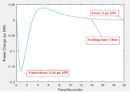
[image:55.612.110.531.340.638.2]In analysis of closed loop LFC system, it is important to analyze tie-line power exchange bevahiour. Figure 2.12 illustrates the deviation in tie-line power exchange between area 1 and 2. This tie line power exchange experiences 0.16pu MW undershoot and settles down after 14 seconds with zero steady state power exchange error. Figure 2.13 shows the deviation in tie-line power exchange between area 2 and 3. This tie line power exchange experiences 0.01pu MW undershoot and settles down after 20 seconds with zero steady state power exchange error. Figure 2.14 shows the deviation in tie-line power exchange between area 1 and 3. Tie-line power exchange bevahiour is upon mutual agreement of the control areas.
41
[image:56.612.107.536.73.342.2]Figure 2.13: Tie-line response of feedback three area LFC system with integral control for area 2 and 3
[image:56.612.101.532.387.662.2]
42
2.5 Feedback N area generalization using integral control
In this chapter, effect of integral control has been analyzed in details. Based on the analysis performed on output response of single area, two area, and three area system, it is concluded that addition of integral control can improve the system performance in terms of steady state error and settling time; however, there is an increase in undershoot/overshoot. This is one of the shortcomings of conventional PID control. The same conclusion is applied to N area LFC system. Hence, a more reliable type of control is needed since power generation system is a system with high level of complexity and uncertainties. Following is list of outputs of multiple area system:
Single Area: Δ𝑓𝑓1
Two Area: Δ𝑓𝑓1, Δ𝑓𝑓2, Δ𝑃𝑃𝑡𝑡𝑖𝑖𝑡𝑡,12
Three Area: Δ𝑓𝑓1, Δ𝑓𝑓2, Δ𝑓𝑓3, Δ𝑃𝑃𝑡𝑡𝑖𝑖𝑡𝑡,12, Δ𝑃𝑃𝑡𝑡𝑖𝑖𝑡𝑡,23, 𝑃𝑃𝑡𝑡𝑖𝑖𝑡𝑡,13
Four Area: Δ𝑓𝑓1, Δ𝑓𝑓2, Δ𝑓𝑓3, Δ𝑓𝑓4, Δ𝑃𝑃𝑡𝑡𝑖𝑖𝑡𝑡,12, 𝑃𝑃𝑡𝑡𝑖𝑖𝑡𝑡,13, 𝑃𝑃𝑡𝑡𝑖𝑖𝑡𝑡,14, 𝑃𝑃𝑡𝑡𝑖𝑖𝑡𝑡,23, 𝑃𝑃𝑡𝑡𝑖𝑖𝑡𝑡,24, 𝑃𝑃𝑡𝑡𝑖𝑖𝑡𝑡,34
43
Chapter 3: Feedback Modelling and Simulation of Power
System Using Adaptive Fuzzy Control
3.1 Introduction to fuzzy logic
Fuzzy Logic (FL) developed by Dr. Zadeh, in 1960s, is able to provide a systematic way for the application of uncertain and indefinite models when precise definition or mathematical representation of the system is unavailable [9].
FL is used in weather forecasting system since global climate is unpredictably changing and airports need to be informed of the changes every instant of time. FL is also used in biological processes such as production of drugs. Many techniques have been used for controlling and automating biological processes; however, they were unsuccessful because of lack of information in some of the biological reactions, complexity of mathematical modelling of the systems, and unavailability of sensors. FL is used in some home appliances such as washing machines. For washing machines, sensors continually monitor conditions inside the machine and accordingly adjust the setting for the best wash result. FL is used in transportation system in Japan. Sendai trains in Japan include FL control for smart transmission, breaking system, traffic planning, predicting number of customers, and energy consumption. FL led to tremendous improvement in autonomous robotics control systems. In 1990s, Motorola produced a FL based microcontroller that was well suited for designing autonomous robots.
Power system is a time-variant system that is influenced significantly by disturbances experienced by each control area. Power system is highly affected by non-internal factors such as weather and season. Modelling a time varying system is a very challenging task [10]. FL theory based control is able to upgrade system performance without the need of mathematical modeling of the system. It is enough to have only some knowledge about the system and its behavior.
44
A = {(x, mA(x)), x ε X)} (3.1) Fuzzy sets are functions that map a value that might be a member of a set to a number between zero and one indicating its actual degree of membership. Fuzzy sets produce a membership curve.
3.2 Fuzzy logic control
As it was shown in chapter 2, conventional controls could not improve the system performance significantly especially in terms of undershoot/overshoot percentage. Even though, the steady state error reduced to zero and the settling time decreased to about 2 seconds, the system behavior was still unacceptable due to high undershoot. Hence, there is need for a more reliable control method to enhance the system performance [9].
FL control can be more effective than conventional control in controlling large scale systems. FL control is used to minimize fluctuation on the system outputs [12]. Combination of the two types of controls can result in a reliable and efficient control design. There exist two types of FL control:
1. Static Fuzzy Control: This control is used when structure and parameters of the FL control are fixed and do not change during real time operation [10].
2. Adaptive Fuzzy Logic Control: This control is used when structure and parameters of FL control change during real time operation. This type of control is more expensive to implement; however, it results in better performance and less mathematical information about the system is needed [10].
Objective of using adaptive FL control is to control the system in the presence of uncertainties and unknown variations. adaptive FL control is difficult to analyze because it is time varying; however, it ensures more desired performance in comparison to static FL control.
Figure 3.1 shows block diagram of a FL control which consists of the following 4 components [10]:
45
2. Inference Mechanism: It selects relevant rules at the current time and decides what the output of the control should be. Output of the control u(t) is input of the plant. 3. Fuzzification: It converts control’s input into information that can be used in
inference mechanism.
4. Difuzzification: It converts output of the control into values that can be used by the plant. Fuzzification and difuzzification are inverse processes.
Figure 3.1: Fuzzy logic control block diagram
By analyzing Figure 3.1, it can be observed that the steady state error is e(t)= r(t) – y(t). FL control has 2 inputs as shown below:
Input 1: e(t) = y(t) - r(t) > ACE (3.2)
Input 2: 𝑑𝑑
𝑑𝑑𝑡𝑡 𝑒𝑒(𝑡𝑡) = 𝑒𝑒(𝑡𝑡̇ ) > 𝐴𝐴𝐴𝐴𝐴𝐴̇ (3.3) If reference input r(t) is zero, then inputs of FL control will be:
Input 1: e(t) = y(t) > ACE (3.4)
Input 2: 𝑑𝑑
𝑑𝑑𝑡𝑡 𝑒𝑒(𝑡𝑡) = 𝑒𝑒(𝑡𝑡̇ ) = 𝑦𝑦(𝑡𝑡̇ ) > 𝐴𝐴𝐴𝐴𝐴𝐴̇ (3.5) To create a fuzzy logic system, following steps must to be taken [13]:
46
2. Define output of the control: Output = control output – plant input
3. Create membership functions: Membership functions are developed based on designer’s knowledge and experience about the system. Membership functions are used to define fuzzy rules.
4. Create rules: Fuzzy rules are defined using IF-THEN relationships. They need to be manually tuned or adjusted in order to obtain the desired system response.
5. Simulate the result: SIMULINK is used to simulate the output result.
3.3 Feedback single area modelling and simulation using adaptive
fuzzy logic control
The inputs of the FL control shown in Equations 3.4 ad 3.5 can be classified into membership functions. Here, the inputs are classified into 7 membership functions as described below: NB: Negative Big, NM: Negative Medium, NS: Negative Small, ZZ: Zero, PS: Positive Small, MP: Positive Medium, PB: Positive Big. These 7 membership functions lead to 49 fuzzy rules as shown in Table 3.1.
Membership functions must be symmetrical and each membership function overlaps with the adjacent functions by 50%. Membership functions are normalized in the interval [-L, L] which is symmetric around zero [13]. The two inputs are combined together using AND operation. Table 3.1 is constructed based on experience and knowledge known about power systems.
Table 3.1: Fuzzy rules for LFC system
𝒆𝒆
(
𝒕𝒕
̇
)
AND NB NM NS ZZ PS PM PB
e(t)
NB NB NB NB NB NM NS ZZ
NM NB NM NM NM NS ZZ PS
NS NM NS NS NS ZZ PS PM
Z NB NM NS ZZ PS PM PB
PS NM NS ZZ PS PS PS PM
PM NS ZZ PS PM PM PM PS
47
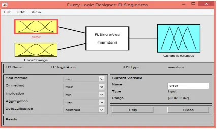
[image:62.612.111.537.185.706.2]Fuzzy Inference System (FIS) in MATLAB is able to design a FL control based on the fuzzy rules defined in Table 3.1. Figures 3.2- 3.5 show the important windows of FIS used in control design. The FL control has two inputs: e(t) and 𝑒𝑒(𝑡𝑡̇ ). Centeroid method is used to defuzzificate the values. The range of each membership, shown in Figure 3.3, is defined based on human’s experience and knowledge about power system.
[image:62.612.112.539.186.443.2]Figure 3.2: FIS - inputs and output
48
[image:63.612.109.536.66.703.2]Figure 3.4: FIS - fuzzy rules
49
To have a stable closed loop system after implementation of FL control, controllability and observability are very important factors. Fuzzy logic control guarantees a closed loop globally stable system if the corresponding open loop system is controllable, observable, and stable [13]. Hence, the system shown in Figure 1.4, which has order of 4, is checked for the above conditions:
1. The system is controllable. The rank of controllability matrix is 4. 2. The system is unobservable. The rank of observability matrix is 3. 3. The system is stable since all the four poles lie on the left half plane.
Hence, the system considered in Figure 1.4 is not a valid candidate for implementation of FL control since it is not observable. As shown in chapter 2, this system worked perfectly fine for implementation of conventional PID control; however, it will not serve the purpose for implementation of FL control. Therefore, in order to illustrate how power system can be controlled using FL control, a different system must be considered. After careful investigation, a system that meets all the above specifications is selected.
The system shown in Figure 3.6 is the open loop system used in this chapter. The LFC system is modelled using state space representation. The poles of the system are located on the left half plane which indicates the system is stable. Rank of controllability and observability matrices are both 3 which is equal to number of state variables used in the system modelling. Hence, the system is controllable, observable, and a valid candidate for FL control implementation.
50
The state space representation of the system, shown in Figure 3.6, is given as follows.
The system has 2 inputs: Δ𝑃𝑃𝑐𝑐 and Δ𝑃𝑃𝑑𝑑. However, only Δ𝑃𝑃𝑑𝑑 is considered as input since disturbance is non-controlling factor. The input is taken as unit step function. The output of the system is frequency deviation of the generator which corresponds to the state variable 𝑋𝑋1.
A=
− −
− −
10 0
200
3 . 0
1 3 . 0
1 0
0 1 . 0 1 . 0
, B=
−
0 0
1 . 0
C=
[
1 0 0]
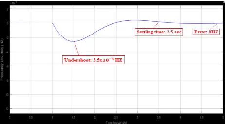
[image:65.612.113.501.377.654.2]Figure 3.7 shows the output response of the open loop single area model illustrated in Figure 3.6. The system is stable with settling time of 3.5 seconds and undershoot of 0.06HZ. The steady state error is about 0.048HZ. Based on the specifications mentioned in section 2.1, the system is expected to have steady state error of no more than 0.01HZ and settling time of less than 3 seconds. The objective in this chapter is to combine implementation of adaptive FL control with a conventional PID control to improve the LFC system performance.
51
Figure 3.8 is block diagram of the feedback single area system used in this chapter. The FL control and PI control are combined together in parallel to improve the system behavior. The system has only one input Δ𝑃𝑃𝑑𝑑 and one output Δ𝑓𝑓.
Figure 3.8: Block diagram of feedback single area LFC system with adaptive FL and PI control
Parameters of the PI control have been tuned carefully to ensure the requirements are met. Table 3.2 shows the parameters of the PI control implemented in Figure 3.8.
Area number (N)
Type of control
Proportional gain constant (𝑲𝑲𝒑𝒑)
Integral gain constant (𝑲𝑲𝒊𝒊)
Frequency bias factor (𝑩𝑩𝑵𝑵)
1 PI -0.25 -3.5 3.5
Table 3.2: Control parameters for feedback single area LFC system with adaptive FL control
52
Figure 3.9: Output response of feedback single area LFC system with adaptive FL and PI control
3.4 Feedback two area modelling and simulation using adaptive
fuzzy logic control
Figure 3.10 shows LFC two area system that is constructed by combining two different control areas. Order of the system is 8 since 8 state variables are needed to model the system. The rank of controllability and observability matrices is 8 which imply the open loop system is controllable and observable, respectively. All the eight poles lie on the left half plane which implies the stability of the system. The system is controllable, observable, and stable; hence, the proposed LFC system is a valid candidate for implementation of FL control.
53
[image:68.612.74.537.404.689.2]Figure 3.10: Block diagram of open loop two area LFC system
54
Figure 3.12: Output response of area 2 in open loop two area LFC system
[image:69.612.76.552.398.690.2]55
Figure 3.14 shows the block diagram of the closed loop two area LFC system. Adaptive FL and PI control are combined together to improve the system performance. Equations 3.6 and 3.7 show ACE of each area:
Area 1: 𝐴𝐴𝐴𝐴𝐴𝐴1 = 𝐵𝐵1.Δ𝜔𝜔1+ Δ𝑃𝑃𝑡𝑡𝑖𝑖𝑡𝑡,12 (3.6)
Area 2: 𝐴𝐴𝐴𝐴𝐴𝐴2 = 𝐵𝐵2.Δ𝜔𝜔2- Δ𝑃𝑃𝑡𝑡𝑖𝑖𝑡𝑡,12 (3.7)
The parameters of the PI control for area 1 and area 2 are selected after numerous trials and careful considerations. Table 3.3 shows the parameters used in PI control design in this section.
Area number (N)
Type of control
Proportional gain constant (𝑲𝑲𝒑𝒑)
Integral gain constant (𝑲𝑲𝒊𝒊)
Frequency bias factor (𝑩𝑩𝑵𝑵)
1 PI -0.02 -1.1 3.5
[image:70.612.77.569.392.664.2]2 PI -1.2 -0.35 2.0
Table 3.3: Control parameters for feedback two area LFC system with adaptive FL control
56
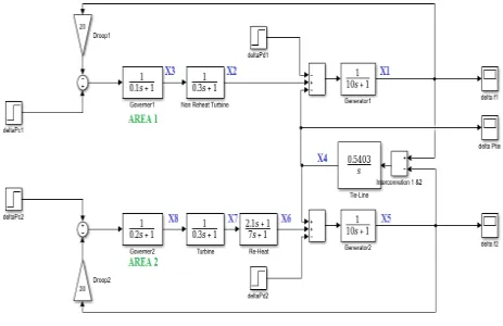
[image:71.612.74.539.225.503.2]Figures 3.15 and 3.16 illustrate the output response of the LFC system after implementation of adaptive FL and PI control. For area 1, the settling time is 3 seconds. The frequency error is 0.0003HZ and the undershoot percentage is 0.059%. For area 2, the settling time is 7.5 seconds. The frequency error is 0.0001HZ and the undershoot percentage is 0.11%. The frequency error and undershoot percentage meet the specifications mentioned in section 2.1. However, the settling time for area 2 needs improvement. Further tuning of FL rules and PI control parameters are required.
Figure 3.15: Output response of area 1 in feedback two area LFC system with adaptive FL and PI control
57
Figure 3.16: Output response of area 2 in feedback two area LFC system with adaptive FL and PI control
[image:72.612.72.540.403.668.2]58