An effective spectral collocation method for the
direct solution of high-order ODEs
N. Mai-Duy
∗School of Aerospace, Mechanical and Mechatronic Engineering,
The University of Sydney, NSW 2006, Australia
Submitted to
Commun. Numer. Meth. Engng
, 20/3/2005;
Resubmitted 23/8/2005; Revised 19/10/2005
SUMMARY
This paper reports a new Chebyshev spectral collocation method for directly solving
high-order ordinary differential equations (ODEs). The construction of the
Cheby-shev approximations is based on integration rather than conventional differentiation.
This use of integration allows the multiple boundary conditions to be incorporated
more efficiently. Numerical results show that the proposed formulation significantly
improves the conditioning of the system and yields more accurate results and faster
convergence rates than conventional formulations.
KEY WORDS: spectral collocation methods; high-order ordinary differential
equa-tions; multiple boundary condiequa-tions; integrated basis-functions
1
INTRODUCTION
Spectral methods are one of the principal methods of discretization for the
numer-ical solution of differential equations. The main advantage of these methods lies in
their accuracy for a given number of unknowns. For smooth problems in simple
ge-ometries, they offer exponential rates of convergence/spectral accuracy. In contrast,
finite-difference and finite-element methods yield only algebraic convergence rates.
The three most widely used spectral versions are the Galerkin, collocation, and tau
methods. The theory and application of spectral methods are covered extensively
in review articles and monographs, see for example [1-5].
High-order ODEs arise in many applications. Examples include the transverse
vi-bration of a uniform beam that can be modelled by a fourth-order ODE; the
a horizontal layer of a fluid heated from below under the effect of rotation and/or a
magnetic field by a sixth-, eighth-, tenth- or twelfth-order ODE [9-11].
There is a relatively small literature on spectral methods for the direct solution of
such high-order problems. In solving a high-order ODE without splitting it into a
set of low-order ODEs, one needs to concern the treatment of multiple boundary
conditions. In the context of the spectral collocation method, there are three basic
approaches to implementing the multiple boundary conditions.
Conventional approach 1 (CA1): This approach modifies the basis functions to incorporate the boundary conditions, see e.g. [4]. For example, in solving the
clamped-clamped-beam eigenvalue problem, one can multiply interpolating
polyno-mials by (1−x2); the solution procedure then becomes simple: (i) to collocate the
governing equation at the interior points and (ii) to remove the first and last columns
of the obtained system. However, it is difficult to apply this approach to problems
involving complicated boundary conditions.
Conventional approach 2 (CA2): This approach takes fewer nodes from the data set to collocate the differential equation, see e.g. [4]. Let p be the order of a
high-order ODE (also the number of boundary conditions) and (N + 1) be the number
of grid points. The ODE is approximated only at the (N + 1−p) points. Apart
from the two boundary points, the question here is which grid points are further
put aside. The performance of the spectral collocation method can depend on the
choice of such points. On the other hand, the implementation of this approach is
straightforward.
Conventional approach 3 (CA3): This approach uses fictitious points as addi-tional unknowns, see e.g. [3]. A set of (p−2) fictitious nodes is added to the original
Chebyshev series expansion can be seen as the Lagrange interpolation polynomial
based on the collocation points, one can construct the Chebyshev differentiation
matrices using the recurrence finite-difference formulae on arbitrarily spaced grids
[3]. Like the case of second-order ODEs, the high-order ODE is forced to be
sat-isfied exactly at the interior points. Since the unknown vector is larger, it allows
one to add (p−2) additional equations to the main system to impose the multiple
boundary conditions. This approach requires a larger set of data points. However, it
provides proper implementation of the multiple boundary conditions and overcomes
difficulties encountered in the first approach.
Recently, in the context of radial-basis-function networks, a new collocation
for-mulation based on integration for solving high-order ODEs was proposed [12]. In
this study, this formulation is extended to the case of Chebyshev polynomials. The
Chebyshev approximations of the dependent variable and its derivatives are
con-structed through an integration process; the integration constants are exploited to
deal with the multiple boundary conditions. There is no need here to introduce
fic-titious points or to reduce the number of nodes used for collocating the ODE. The
proposed Chebyshev collocation method is applicable to general high-order ODEs,
where these equations can have variable coefficients, nonlinear terms,
nonhomoge-neous terms, complicated boundary conditions and numerous different derivatives.
The method is verified through the solution of such ODEs governing initial-value,
boundary-value and eigenvalue problems. Among those are the free vibration of a
nonuniform ring, the free vibration of a uniform beam, and the Hamel flow problem
that have a wide range of applications in engineering. Numerical results show that
the proposed approach outperforms conventional approaches regarding the
condi-tioning of the system, accuracy and convergence rate.
The remainder of the paper is organized as follows. In section 2, a brief review of the
integration for directly solving high-order ODEs is presented in section 3. In section
4, the proposed method is verified through the solution of various problems governed
by ODEs of the second-, fourth-, sixth-, eighth- and twelfth-orders. Section 5 gives
some concluding remarks.
2
CHEBYSHEV POLYNOMIALS
The Chebyshev polynomial of first kindTk(x) is defined by
Tk(x) = cos(karccos(x)), k = 0,1,2,· · · , (1)
where−1≤x≤1. The polynomial Tk(x) can be expanded in power series as
T0(x) = 1, (2)
Tk(x) =
k
2
[k/2] X
m=0
(−1)m2
k−2m(k−m−1)!
m!(k−2m)! x
k−2m, k >0, (3)
where [k/2] is the integer part ofk/2.
3
THE SPECTRAL COLLOCATION METHOD
Consider the following ODE
Lu=f, a≤x≤b, (4)
where L is a differential operator and f is a given function. This equation is
initial-value/boundary-spaced Gauss-Lobatto (G-L) points
{xi}Ni=0 = cos πi N N i=0 (5)
which cluster at boundaries.
3.1
Conventional differentiation-based formulations (CDFs)
An approximate solutionu(x) is sought in the truncated Chebyshev series form
u(x) =
N
X
k=0
akTk(x), (6)
where{ak}Nk=0 is the set of expansion coefficients to be found. Thepth-order
deriva-tive of the variable u is then obtained through differentiation as
dpu(x)
dxp = N
X
k=0
ak
dpT k(x)
dxp . (7)
The use of G-L points (5) allows a fast Fourier transform to be employed to shift
between spectral space{ak}Nk=0 and physical space{ui}Ni=0:
ak=
2
N¯ck N X i=0 1 ¯ ci
uiTk(xi), (8)
The evaluation of the derivatives (7) at the G-L points yields
c
du dx =D
(1)bu=Dbu, (9)
d
d2u
dx2 =D
(2)bu=D2u,b (10)
· · · ·
d
dpu
dxp =D
(p)bu=Dpu,b (11)
where the symbolb. is used to denote a vector, e.g., ub= (u(x0), u(x1),· · · , u(xN))T
and
c
dpu
dxp =
dpu
dxp(x0),
dpu
dxp(x1),· · · ,
dpu
dxp(xN)
T
, and D(.) are the differentiation matrices.
The entries of D (D(1)) are given by
Dij =
¯
ci
¯
cj
(−1)i+j
xi−xj
, 0≤i, j ≤N, i6=j, (12)
Dii=−
xi
2(1−x2
i)
, 1≤i≤N −1, (13)
D11=−DN N =
2N2+ 1
6 . (14)
As an alternative approach, the diagonal entries of D can be computed in the way that represents exactly the derivative of a constant [13]
Dii =− N
X
j=0,j6=i
Dij. (15)
Higher-order derivatives D(p) can be constructed using recursions, see e.g. [3,14], which are faster and more numerically stable. The roundoff properties of the spectral
differentiation matrices were studied in, e.g., [13,15].
Using the above expressions, the ODE can be transformed into a set of algebraic
that was briefly reviewed earlier. The obtained system is then solved for the values
of the variable u at the grid points. There are a number of software packages
implementing spectral methods. Among them are MATLAB packages by Trefethen
[4] and Weideman and Reddy [16]. The former and Fornberg’s recursion codes used
for finding finite-difference weights on arbitrarily spaced grids [3] are employed in
the present work for calculating the CDF case.
3.2
The proposed integration-based formulation (PIF)
For the proposed formulation, the highest-order derivativedpu/dxp in the differential
equation is sought in the truncated Chebyshev series form
dpu(x)
dxp = N
X
k=0
akTk(x). (16)
Expressions for lower derivatives and the variable itself are then obtained through
integration as
dp−1u(x)
dxp−1 =
N
X
k=0
akIk(p−1)(x) +c1, (17)
dp−2u(x)
dxp−2 =
N
X
k=0
akIk(p−2)(x) +c1x+c2, (18)
· · · ·
du(x)
dx =
N
X
k=0
akIk(1)(x) +c1
xp−2
(p−2)! +c2
xp−3
(p−3)! +· · ·cp−2x+cp−1, (19)
u(x) =
N
X
k=0
akIk(0)(x) +c1
xp−1
(p−1)! +c2
xp−2
(p−2)! +· · ·cp−1x+cp, (20) where Ik(p−1)(x) = R Tk(x)dx, Ik(p−2)(x) =
R
using recurrence relations [5]
Z
T0(x)dx=T1(x), (21) Z
T1(x)dx=
1
4[T0(x) +T2(x)], (22)
Z
Tk(x)dx=
1 2
Tk+1(x)
(k+ 1) −
Tk−1(x)
(k−1)
, k >1, (23)
or integrating (2)-(3) directly, e.g., fork >0:
Ik(p−1)(x) =
Z
Tk(x)dx=
k
2
[k/2] X
m=0
(−1)m2
k−2m(k−m−1)!
m!(k−2m+ 1)! x
k−2m+1, (24)
Ik(p−2)(x) =
Z
Ik(p−1)(x)dx= k 2
[Xk/2]
m=0
(−1)m2
k−2m(k−m−1)!
m!(k−2m+ 2)! x
k−2m+2, (25)
· · · ·
Ik(0)(x) =
Z
Ik(1)(x)dx = k 2
[k/2] X
m=0
(−1)m2
k−2m(k−m−1)!
m!(k−2m+p)! x
k−2m+p. (26)
It can be seen that apart from the Chebyshev coefficients {ak}Nk=0, the PIF
((16)-(20)) produces new coefficients (integration constants{ci}pi=1) whose number is equal
to the order of ODE/the number of boundary conditions, i.e. p. As a result, it allows
one (i) to approximate the ODE at the whole set of G-L points and (ii) to add p
additional equations to the main system to impose p boundary conditions. In this
sense, the PIF makes the implementation of these two parts of the solution procedure
The evaluation of (16)-(20) at the G-L points leads to
d
dpu
dxp =Tbs=I
(p)bs, (27)
d
dp−1u
dxp−1 =I
(p−1)bs, (28)
· · · ·
c
du dx =I
(1)bs, (29)
b
u=I(0)bs, (30)
where bs = (a0, a1,· · ·, aN, c1, c2,· · ·, cp)T and I(p−1),I(p−2),· · · ,I(0) are the known
integration matrices. For convenience of computation, I(p),I(p−1),· · · ,I(1) are
aug-mented using zero-submatrices so that they have the same dimension as I(0).
From (9)-(11) and (27)-(30), it can be seen that the CDF and PIF have similar
discrete approximation forms (D ⇔ I and ub ⇔ bs). Thus, the process of reduc-ing the differential equation to a set of algebraic equations by the PIF is similar
to that by the CDF. A distinct difference between the two formulations in
imple-mentation is that imposition of the multiple boundary conditions is conducted by
means of integration constants (bs is larger than bu) for the PIF and by the
node-reduction/fictitious-point technique for the CDF. Both formulations result in dense
4
NUMERICAL RESULTS
In the following examples, the accuracy of a numerical solution produced by an
approximation scheme is measured via the discrete relativeL2 error defined as
Ne =
sPN
i=0[ue(xi)−u(xi)] 2 PN
i=0ue(xi)2
, (31)
where ue and u are the exact and approximate solutions, respectively. Nonlinear
systems of equations are solved using the Picard-type and Newton-type iteration
schemes. It is noted that the former is relatively easy to implement, but its
conver-gence is often slow.
4.1
Second-order boundary-value problem
The PIF is first tested through the solution of the following second-order ODE
d2u
dx2+sin(x)
du
dx+exp(x)u=−16π
2sin(4πx)+4πsin(x) cos(4πx)+exp(x) [2 + sin(4πx)],
(32)
defined over −1≤x≤1 and subject to the Robin boundary conditions
u(±1) + du(±1)
dx = 2 + 4π.
The exact solution can be verified to be ue = 2 + sin(4πx). Seven data sets,
{10,15,· · · ,40}G-L points, are employed to study this problem. The Robin
bound-ary conditions are imposed explicitly by adding two additional equations to the main
system. Results concerning the conditioning and the discrete relative L2 error
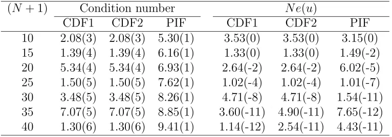
ob-tained by the CDF and PIF are shown in Table 1. For the former, two versions
for-mulaD(2) =D2, while the second one (CDF2) uses the explicit expression of D(2)
[5]. The relative L2 errors obtained by CDF1 and CDF2 are “exactly the same”
for (N + 1) = {10,15,· · · ,30}, but different for (N + 1) = {35,40}. In terms of
accuracy, the PIF produces more accurate results than the CDFs; for example, at
(N+ 1) = 30,Nes are 1.54×10⁻¹¹ (PIF) and 4.71×10⁻⁸ (CDF1,2). In terms of the
conditioning of the system, the PIF yields at least two orders of magnitude lower
than the CDFs; furthermore, when (N + 1) increases from 10 to 40, the condition
number increases from 2.08×10³to 1.30×10⁶for the CDFs, but only from 5.30×101
to 9.41×101 for the PIF. Exponential rates of convergence are achieved for both
formulations. The order of the error, which is defines as Ne =O(N−α), at the first
six sets isO(N−21.58) for the PIF and O(N−18.62) for the CDF1; the PIF case yields
faster convergence.
For the CDF case, if one tries to add an algebraic polynomial (c1x+c2) to (6) in
order to have similar forms as the PIF case, i.e.,
u(x) =
N
X
k=0
akTk(x) +c1x+c2, (33)
du dx =
N
X
k=0
ak
dTk(x)
dx +c1, (34)
d2u
dx2 =
N
X
k=0
ak
d2T
k(x)
dx2 , (35)
the obtained system of equations is singular because the first and last two columns
4.2
Fourth-order problems
4.2.1 Initial-value problem
Consider the following fourth-order initial-value problem
(x3−3x2+ 6x−6)d
4u
dx4 −x 3d3u
dx3 + 3x 2d2u
dx2 −6x
du
dx + 6u= 0, −1≤x≤1, (36)
Initial conditions: u(−1), du(−1) dx ,
d2u(−1)
dx2 ,
d3u(−1)
dx3 ,
Exact solution: ue= exp(x) + 5x3−2x2+x.
The initial values are obtained using the exact solution. Six data sets,{4,6,· · · ,14}
G-L points, are employed. For the CDF case, the three derivative initial conditions
are enforced explicitly by adding three additional equations to the main system. It
is difficult to apply the approach CA1 to this problem; only the two approaches CA2
and CA3 are employed here. Results concerning the condition number and accuracy
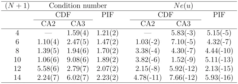
obtained by the proposed and conventional approaches are given in Table 2. The
PIF significantly improves the conditioning of the system over the CDFs, e.g., 2
orders of magnitude for the coarsest grid and 5 orders of magnitude for the finest
grid. Furthermore, the PIF yields the most accurate results, followed by the CA3
and then CA2; for example, at (N+ 1) = 12, Nes are 2.13×10⁻¹⁵, 5.92×10⁻¹² and
2.15×10⁻⁸, respectively. The results of the CA2 are less accurate (a few orders of
magnitude greater), probably due to the fact that the ODE is not approximated at
every interior point. On the other hand, all approaches feature exponential rates of
convergence. The orders of the relativeL2 error measured at (N+ 1) ={6,8,10,12}
areO(N−24.32),O(N−20.52) andO(N−16.29) for the PIF, CA3 and CA2, respectively;
4.2.2 Boundary-value problem - Hamel flow problem
A steady-state two-dimensional flow in the region between two semi-infinite plane
walls set at an angle 2α is known as the Hamel flow problem [17]. It is convenient
to use polar co-ordinates (r, θ) where r is measured from the intersection of the two
walls and θ is measured from the centreline of the duct. The inward flow, which is
driven by a steady line sink at the apex, is assumed to be purely radial along the
lines θ=constant (−α ≤ θ ≤ α). Since the stream function ψ depends only on θ,
the dimensionless governing equation for the Hamel flow can be written as
d4ψ
dθ4 + 4
d2ψ
dθ2 −2Re
dψ dθ
d2ψ
dθ2 = 0, (37)
subject to the boundary conditions
ψ(±α) =±1, and dψ(±α)
dθ = 0,
whereReis the Reynolds number. For creeping flow (Re= 0) and viscous flow with
very large values ofRe, they can be solved analytically and their solutions are given
by
ur(θ)
ur(0)
= cos(2θ)−cos(2α)
1−cos(2α) (Re= 0), (38)
ur(θ)
ur(0)
= 3 tanh2(0.5αRe)0.5(1− |θ|/α) + tanh−1(2/3)0.5−2 (Re≫), (39)
whereur is the radial velocity defined as ur =−1r∂ψ∂θ. More details can be found in
[17].
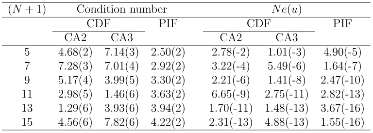
The domain of interest isθ ∈[−α, α] = [−π/6, π/6]. For creeping flow, six data sets,
{5,7,· · · ,15}G-L points, are employed. The conditioning and accuracy obtained by
formulations are similar to the previous problem. For viscous flow, this fourth-order
ODE is nonlinear and hence must be solved iteratively. The nonlinearity is handled
here using trust-region methods that retain two attractive features, namely rapid
local convergence of the Newton iteration scheme and strong global convergence of
the Cauchy method [18]. It is noted that Newton’s method can run into difficulties if
the starting point is far from the solution and the Jacobian matrix is ill-conditioned.
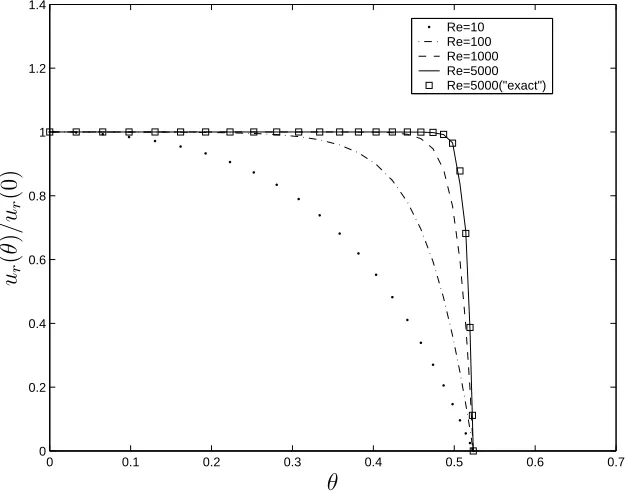
A range of Re= {0,10,50,100,1000,5000} is considered. The computed solutions
at the lower and nearest value of Re are utilized as an initial guess. The
radial-velocity profiles obtained by the present formulation for various Reynolds numbers
using 51 G-L points are plotted in Figure 1. The computed results at Re = 5000
are compared to those obtained using (39); good agreement can be seen. When the
Reynolds number increases, the velocity magnitude becomes nearly constant except
near the plate walls, forming boundary layers of thickness O(pα/Re) (Figure 1).
4.2.3 Eigenvalue problem - Free vibration of a uniform beam
The PIF is further verified through the solution of fourth-order eigenvalue problems
subject to various types of boundary conditions. Consider the free lateral vibration
of a uniform beam. The non-dimensional governing equation can be written as
d4φ
dx4 =λφ, 0≤x≤1, (40)
and the boundary conditions are given by
φ(0) =φ′(0) =φ(1) =φ′(1) = 0, for a clamped-clamped beam (CC), (41)
φ(0) =φ′(0) =φ(1) =φ′′(1) = 0, for a clamped-hinged beam (CH), (42)
where λ is the eigenvalue and φ is the eigenfunction. Exact solutions are found by
solving the frequency equations
cos(λ) cosh(λ) = 1, (CC), (44)
tan(λ)−tanh(λ) = 0, (CH), (45)
sin(λ) = 0, λ=nπ, (HH). (46)
Discretizing (40) at the whole set of G-L points and implementing the boundary
conditions (41), (42) or (43) constitute the following two subsets of equations
Aa−λ4Ba = 0, (47)
Ca = 0, (48)
or
(A1,A2)(a1,a2)T −λ4(B1,B2)(a1,a2)T = 0, (49)
(C1,C2)(a1,a2)T = 0, (50)
where A1 and B1 are matrices of dimension (N + 1)× (N + 1), A2 and B2 of
(N + 1)×4, C1 of 4×(N + 1), C2 of 4×4, a1 of 1×(N + 1), and a2 of 1×4.
After performing some algebraic manipulation, the above system of equations takes
the form
[(A1−A2C−21C1)−λ4(B1−B2C−21C1)]aT1 =0. (51)
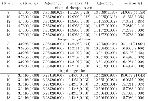
A simple coordinate transformation ([0,1] → [−1,1]) is carried out. Results
con-cerning λk, k = 1,· · · ,5, are shown in Table 4. Very accurate results and fast
convergence are achieved. For example, the percentage errors for the case of a
hinged-hinged beam using 18 grid points are 2.8×10⁻¹⁴, 1.4×10⁻¹⁴, 4.5×10⁻¹²,
3.7×10⁻¹⁰ and 1.3×10⁻⁷% for λ
4.3
Sixth-order eigenvalue problem - Free vibration of a ring
The vibrational behaviour of a ring-like structure governed by a sixth-order ODE
[6,7] is considered in this section. A ring has rectangular cross-sections of constant
width and parabolically variable thickness. The case of normal, in-plane modes of
vibration is studied here, where one disregards stretching in the axial direction.
4.3.1 A circular ring with supports
In this case, the non-dimensional governing equation is given by
β1v[6]+β2v[5] +β3v[4] +β4v ′′′
+β5v ′′
+β6v ′
−Ω2f v′′+f′v′ −π2f v= 0, (52)
0≤α≤1,
subject to the boundary conditions
v(0) =v′(0) =v′′′(0) = 0, v(1) =v′(1) =v′′′(1) = 0,
where v[q] =dqv/dαq, v is the tangential displacement, α is the dimensionless
vari-able, Ω is the dimensionless frequency and
β1 = φ/π4, β2 = 3φ ′
/π4, β3 = (2φ/π2) + (3φ ′′
/π4),
β4 = (4φ ′
/π2) + (φ′′′/π4), β5 =φ+ (3φ ′′
/π2), β6 =φ ′
+ (φ′′′/π2),
φ = [f(α)]3, f(α) = −4(r−1)α2+ 4(r−1)α+ 1,
in which r is the variable related to the thickness of the cross-section of the ring.
The variable coefficients in (52) involve sixth-order polynomials in α. The solution
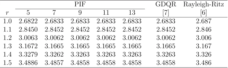
is omitted here for brevity. Six data sets, {7,9,· · · ,17} G-L points, are employed.
The fundamental frequencies obtained are listed in Table 5. The corresponding
values predicted by the optimized Rayleigh-Ritz method [6] and the GDQR method
[7] are also given for comparison purpose. They are in good agreement. The present
method achieves highly accurate results using considerably small numbers of grid
points. Forr= 1.5, at least 4 significant digits remain constant when (N+ 1)≥13.
4.3.2 A completely free ring
In this case, the non-dimensional governing equation is given by
β1v[6]+β2v[5]+β3v[4]+β4v ′′′
+β5v ′′
+β6v ′
−Ω2f v′′
+f′v′ −π2f v/4= 0,
(53)
0≤α≤1,
subject to the boundary conditions
v(0) = v′′(0) = 0, φ′(0)hv′(0) + 4v′′′(0)/π2i+ 4φ(0)v[4](0)/π2 = 0,
v(1) = v′′(1) = 0, φ′(1)hv′(1) + 4v′′′(1)/π2i+ 4φ(1)v[4](1)/π2 = 0,
where
β1 = 16φ/π4, β2 = 48φ ′
/π4, β3 = (8φ/π2) + (48φ ′′
/π4),
β4 = (16φ ′
/π2) + (16φ′′′/π4), β5 =φ+ (12φ ′′
/π2), β6 =φ ′
+ (4φ′′′/π2),
φ = [f(α)]3, f(α) = −(r−1)α2+ 2(r−1)α+ 1.
Five data sets,{5,7,· · · ,13} G-L points, are employed. Table 6 displays the
the GDQR [7] and Rayleigh-Ritz [6] methods, where good agreement can be seen.
Highly accurate results are achieved. Forr= 1.5, at least 4 significant digits remain
constant when (N + 1)≥9.
4.4
Eighth-order boundary-value problem
The governing equation and boundary conditions are, respectively, given by
d8u
dx8 = 7!
exp(−8u)− 2 (1 +x)8
, a= 0 ≤x≤b=√e−1, (54)
u(a) = 0, u(b) = 1/2,
u[2i](a) =−(2i−1)!, u[2i](b) =−(2i−1)!e−i, i= 1,2,3,
for which the exact solution isue = ln(1 +x). This nonlinear problem is taken from
[10]. A Picard-type iteration is employed to render the nonlinear term linear. Eleven
data sets,{6,8,· · · ,26}G-L points, are employed. For this high-order problem, the
condition numbers of the system matrix obtained by the CA2 and CA3 are very
large (Table 7). It is remarkable that the condition numbers obtained for the PIF
case only have the order of 104 for all the data sets. The relative L
2 errors are of
O(10−3)−O(10−6),O(10−4)−O(10−9) and O(10−6)−O(10−16) for the CA2, CA3
and PIF, respectively; the PIF is far superior to the CA2 and CA3.
4.5
Twelfth-order boundary-value ODE
This problem is taken from [11], where the governing equation is
d12u
dx12 = 11!
exp(−12u)− 2 (1 +x)12
and the boundary conditions are
u(a) = 0, u(b) = 1/3,
u[2i](a) = −(2i−1)!, u[2i](b) = −(2i−1)!e−2i/3, i= 1,· · · ,5,
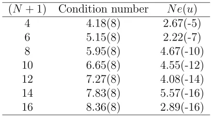
for which the exact solution is ue = ln(1 +x). For this very high-order problem,
the two approaches CA2 and CA3 fail to obtain a converged solution since their
matrices are close to singular; for example, at (N + 1) = 4, the conditioning of the
system of the CA3 is already up to 2.77×10¹⁶. Table 8 presents the conditioning
of the system and the accuracy of the solution obtained by the PIF; an exponential
rate of convergence is achieved.
5
CONCLUDING REMARKS
This paper presents a new Chebyshev spectral collocation method for directly solving
high-order ODEs. The Chebyshev expressions representing the dependent variable
and its derivatives are constructed through an integration process. This use of
integration provides an effective way to implement the multiple boundary conditions,
without the need to introduce fictitious points or the need to reduce the number
of nodes used for discretizing the ODE. It works in a similar fashion for different
types of the boundary condition and different orders of the ODE. The proposed
method appears to be particularly well suited to problems governed by very
high-order ODEs. Numerical results show that its performance is superior to those of
conventional methods in terms of the conditioning of the system, accuracy and
convergence rate.
The author would like to thank the referees for their helpful comments.
REFERENCES
1. Gottlieb D, Orszag SA. Numerical Analysis of Spectral Methods: Theory and
Applications. SIAM: Philadelphia, 1977.
2. Canuto C, Hussaini MY, Quarteroni A, Zang TA. Spectral Methods in Fluid
Dynamics. Springer-Verlag: New York, 1988.
3. Fornberg B. A Practical Guide to Pseudospectral Methods. Cambridge
Uni-versity Press: Cambridge, 1998.
4. Trefethen LN. Spectral Methods in MATLAB. SIAM: Philadelphia, 2000.
5. Peyret R.Spectral Methods for Incompressible Viscous Flow. Springer-Verlag:
New York, 2002.
6. Gutierrez RH, Laura PAA. Vibrations of non-uniform rings studied by means
of the differential quadrature method. Journal of Sound and Vibration 1995;
185(3): 507–513.
7. Wu TY, Liu GR. Application of generalized differential quadrature rule to
sixth-order differential equations. Communications in Numerical Methods in
Engineering 2000; 16: 777–784.
8. Kelkar VS, Sewell RT.Fundamentals of the Analysis and Design of Shell
Struc-tures. Prentice-Hall: New Jersey, 1987.
9. Chandrasekhar S. Hydrodynamic and Hydromagnetic Stability. Oxford
10. Boutayeb A, Twizell EH. Finite-difference methods for the solution of special
eighth-order boundary-value problems. International Journal of Computer
Mathematics 1993,48: 63–75.
11. Boutayeb A, Twizell EH. Finite-difference methods for twelfth-order
boundary-value problems. Journal of Computational and Applied Mathematics1991,35: 133–138.
12. Mai-Duy N. Solving high order ordinary differential equations with radial basis
function networks. International Journal for Numerical Methods in
Engineer-ing 2005,62: 824–852.
13. Bayliss A, Class A, Matkowsky BJ. Roundoff error in computing derivatives
using the Chebyshev differentiation matrix. Journal of Computational Physics
1995, 116(2): 380–383
14. Welfert BD. Generation of pseudospectral differentiation matrices I. SIAM
Journal on Numerical Analysis 1997, 34(4): 1640–1657.
15. Baltensperger R, Trummer MR. Spectral differencing with a twist. SIAM
Journal on Scientific Computing 2003, 24(5): 1465–1487.
16. Weideman JAC, Reddy SC. A MATLAB differentiation matrix suite. ACM
Transactions on Mathematical Software 2000, 26(4): 465–519.
17. Batchelor GK. An Introduction to Fluid Dynamics. Cambridge University
Press: Cambridge, 1967.
18. McCartin BJ. A model-trust region algorithm utilizing a quadratic interpolant.
Table 1: Second-order boundary-value problem: Conditioning and accuracy. Note that a(b) means a×10b.
(N + 1) Condition number N e(u)
Table 2: Fourth-order initial-value problem: Conditioning and accuracy (for the CA2 case, two interior points x1 and xN−1 are put aside; for the CA3 case, two
fictitious points are set to ±1.1).
(N + 1) Condition number N e(u)
CDF PIF CDF PIF
CA2 CA3 CA2 CA3
Table 3: Fourth-order boundary value problem, Hamel flow, Re= 0: Conditioning and accuracy (for the CA2 case, two interior pointsx1 and xN−1 are put aside; for
the CA3 case, two fictitious points are set to ±1.1).
(N + 1) Condition number N e(u)
CDF PIF CDF PIF
CA2 CA3 CA2 CA3
Table 4: Fourth-order eigenvalue problem, free vibration of a uniform beam: eigen-values obtained by the PIF.
(N + 1) λ1(error %) λ2(error %) λ3(error %) λ4(error %) λ5(error %)
clamped-clamped beam
8 4.7300(0.000) 7.8516(0.021) 11.1296(1.218) 13.9699(1.183) 24.9089(44.159) 10 4.7300(0.000) 7.8532(0.000) 10.9992(0.032) 14.0925(0.315) 18.1575(5.085) 12 4.7300(0.000) 7.8532(0.000) 10.9956(0.000) 14.1355(0.012) 17.3471(0.395) 14 4.7300(0.000) 7.8532(0.000) 10.9956(0.000) 14.1371(0.000) 17.2810(0.012) 16 4.7300(0.000) 7.8532(0.000) 10.9956(0.000) 14.1372(0.000) 17.2788(0.000) 18 4.7300(0.000) 7.8532(0.000) 10.9956(0.000) 14.1372(0.000) 17.2788(0.000)
clamped-hinged beam
8 3.9266(0.000) 7.0683(0.003) 10.2606(0.494) 13.2950(0.425) 20.1161(21.964) 10 3.9266(0.000) 7.0686(0.000) 10.2111(0.008) 13.3384(0.100) 16.9003(2.466) 12 3.9266(0.000) 7.0686(0.000) 10.2102(0.000) 13.3514(0.003) 16.5196(0.158) 14 3.9266(0.000) 7.0686(0.000) 10.2102(0.000) 13.3518(0.000) 16.4940(0.003) 16 3.9266(0.000) 7.0686(0.000) 10.2102(0.000) 13.3518(0.000) 16.4934(0.000) 18 3.9266(0.000) 7.0686(0.000) 10.2102(0.000) 13.3518(0.000) 16.4934(0.000)
hinged-hinged beam
Table 5: Sixth-order eigenvalue problem, free vibration of a non-uniform ring with constraints: fundamental frequencies.
PIF GDQR Rayleigh-Ritz
Table 6: Sixth-order eigenvalue problem, free vibration of a non-uniform ring with-out constraints: fundamental frequencies.
PIF GDQR Rayleigh-Ritz
Table 7: Eighth-order boundary-value problem: Conditioning and accuracy (for the CA2 case, 3 interior points adjacent to each boundary are put aside; for the CA3 case, fictitious points are set to {±1.3,±1.2,±1.1}).
(N + 1) Condition number N e(u)
CDF PIF CDF PIF
CA2 CA3 CA2 CA3
Table 8: Twelfth-order boundary-value problem: Conditioning and accuracy of the PIF. Note that the CDF case fails to obtain a converged solution since the system matrices obtained are close to singular. For example, at (N+1) = 4, the conditioning of the system of the CA3 is up to 2.77×10¹⁶.
0 0.1 0.2 0.3 0.4 0.5 0.6 0.7 0
0.2 0.4 0.6 0.8 1 1.2 1.4
Re=10 Re=100 Re=1000 Re=5000 Re=5000("exact")
θ
ur
(
θ
)
/u
r
(0
[image:31.612.139.452.40.286.2])