An integral-collocation-based fictitious-domain technique for solving elliptic problems

(1)

An integral-collocation-based fictitious domain

technique for solving elliptic problems

N. Mai-Duy

∗,†

, H. See

‡

and T. Tran-Cong

†

_{Computational Engineering and Science Research Centre (CESRC)}

The University of Southern Queensland, Toowoomba, QLD 4350, Australia

‡

_{School of Chemical & Biomolecular Engineering}

The University of Sydney, Sydney, NSW 2006, Australia

Submitted to

Commun. Numer. Meth. Engng, 17-Apr-2007; revised,

5-Jun-2007

Short title: FICTITIOUS DOMAIN TECHNIQUE

(2)

SUMMARY

This paper presents a new fictitious-domain technique for numerically solving elliptic second-order partial-differential equations (PDEs) in complex geometries. The pro-posed technique is based on the use of integral collocation schemes and Chebyshev polynomials. The boundary conditions on the actual boundary are implemented by means of integration constants. The method works for both Dirichlet and Neumann boundary conditions. Several test problems are considered to verify the technique. Numerical results show that the present method yields spectral accuracy for smooth (analytic) problems.

KEY WORDS: fictitious domains; point collocation techniques; integrated Cheby-shev polynomials; elliptic problems

1 INTRODUCTION

Solving PDEs in irregularly shaped domains presents a challenge in computational engineering. Well-known techniques used for handling complex geometries include coordinate transformations, domain decompositions, meshless discretizations and fictitious domains. Each technique has some advantages over the others for certain classes of problems.

Fictitious-domain techniques can be traced back to the early 1950s ([1] and refer-ences therein). These techniques have been very successful in solving complicated engineering problems (e.g. [2,3]). The basic idea behind fictitious-domain techniques is to extend domains of complicated shapes to those of simpler shapes for which the generation of meshes is simple and well-established efficient numerical solvers can be applied. Another advantage, when compared with coordinate transformation tech-niques, is that they are able to retain the PDE in a Cartesian form. It is noted that the transformation of the governing equation into generalized curvilinear coordinates that conform with complex boundaries usually introduces an additional error [4]. A main difficulty here lies in the method employed to take into account the boundary conditions. Glowinski et al. [5] have presented a family of fictitious-domain tech-niques which are based on the explicit use of Lagrange multipliers defined on the actual boundary and associated with the boundary conditions for Dirichlet elliptic problems. Since then, the Lagrange multiplier/fictitious-domain methods have be-come increasingly popular. Many further developments and applications have been reported: for instance, for the solution of the Navier-Stokes equations governing incompressible viscous flows (e.g. [6,7]), for the fluid/rigid-body interactions (e.g. [8,3,9]) and for the fluid/flexible-body interactions (e.g. [10]).

Spectral collocation methods/pseudo-spectral methods are global numerical solvers for PDEs and they are known to be very accurate (cf. [11-15]). The methods use a set of orthogonal polynomials such as Chebyshev polynomials (very smooth basis

(3)

functions) to represent the approximate solution of the PDE and take the cosine-type points (the zeros of (1−x2₎_T′

N in whichN is the degree of the polynomial) as the grid points (−1≤x≤1). The conversion of the spectral space into the physical space can be carried out efficiently through a fast Fourier transform. Unlike Galerkin spectral methods, spectral collocation methods approximate the solution in terms of nodal variable values. The main advantages of pseudo-spectral methods lie in their accuracy and economy. For problems whose solutions are smooth (infinitely differ-entiable), they yield an exponential rate of convergence as the grid is refined or the order of the approximation N is increased (spectral accuracy). The interpolation error decreases more rapidly than any power of 1/N [11]. For two-dimensional prob-lems, it requires that the problem domain be rectangular [−1,−1]×[1,1], which, at the beginning, limits the application of pseudo-spectral techniques to problems defined in simple geometries. There has been a considerable effort put into the de-velopment of these techniques in complex geometries. A general and popular way to deal with complex geometries is based on the use of domain decompositions and co-ordinate transformations. The problem domain is divided into several subdomains, and each subdomain is mapped onto the reference square. Orszag [16] has presented a technique for matching approximate solutions over contiguous regions, namely the patching technique. It requires the approximate solution and its first-order normal derivative to be continuous at the subdomain interfaces. Given a fixed number of subdomains, the approximation is still spectral when the grids on subdomains are refined. The patching technique normally provides an approximate solution that is C1 _{function across the internal artificial boundaries. The reader is referred to}

the book of Karniadakis and Sherwin [17] for a detailed discussion of multi-domain spectral methods.

It is well known that integration is a smoothing operator and is more numerically stable than differentiation. The weak forms associated with finite-element techniques and the inverse statements associated with boundary-element techniques are derived from integrating a weighted residual statement by parts once and twice, respectively (cf. [18]). The integration process reduces the required order of continuity of the approximate solution. A weak solution satisfies the governing equation in an average sense. On the other hand, point collocation techniques such as pseudo-spectral and finite-difference methods are directly based on the strong form of the PDE. The main advantage of these techniques lies in their simplicity as there is no integration of the PDE involved. Grids/meshes are only required for the interpolation of the field variable. The governing equation is satisfied in a pointwise sense.

(4)

the integral collocation formulation for the solution of differential equations, with RBFs or Chebyshev polynomials, the constants of integration have been found to be very useful. They provide an alternative way, which is very effective, for the im-plementation of multiple boundary conditions [23-25] and also allow a higher-order smoothness of the approximate solution across the subdomain interfaces [26]. It will be shown that, in the context of fictitious-domain techniques, the constants of integration can be utilized for the purpose of imposing the prescribed conditions on the actual boundary. This work seems to be the first report implementing the idea of fictitious domain in the context of pseudo-spectral methods; it provides a new way of handling irregularly shaped domains. Even in the case where domain decompositions are required, the use of fictitious domains can be seen to be more straightforward to implement than with the use of coordinate transformations. The presently proposed approach is underpinned by three main features, namely the high-order accuracy of the Chebyshev collocation technique, the effective implemen-tation of boundary conditions of the integral collocation formulation, and the ability to deal with irregularly shaped domains of the fictitious-domain technique.

An outline of the paper is as follows. In section 2, a brief review of point collocation formulations is given. The proposed fictitious-domain technique, which is based on the integral collocation formulation, is described in section 3. The method is then verified through the solution of several test problems in section 4; these test examples involve simply-connected domains, multiply-connected domains, multi-domains, Dirichlet boundary conditions, Neumann boundary conditions and singular solutions. Section 5 gives some concluding remarks.

2 POINT COLLOCATION FORMULATIONS

The Chebyshev collocation technique consists in approximating the solution with Chebyshev polynomials, and forcing the differential equation and the boundary con-ditions to be satisfied exactly at the cosine-type points. The construction of the Chebyshev approximations representing the approximate solution of the PDE can be based on differentiation and integration.

2.1 Differential formulation

An approximate function f can be represented by the Chebyshev interpolant of degreeN as follows

f(x) = N

X

k=0

akTk(x) = N

X

k=0

akcos(karccos(x)), (1)

(5)

where −1 ≤ x ≤ 1, {ak}N_k₌₀ are unknown coefficients and {Tk}N_k₌₀ are the Cheby-shev polynomials. Expressions of derivatives of (1) will then be obtained through differentiation.

At the Gauss-Lobatto (G-L) points,

{xi}N_i₌₀ =

cos πi N N i=0 , (2)

the values of derivatives off are simply computed by

cdf

dx =D

(1)_fb₌_D_{f ,}b ₍₃₎

d d2_f

dx2 =D

(2)_f_b₌_D2_{f ,}_b ₍₄₎

· · · ·

d dp_f

dxp =D

(p)_f_b₌_Dp_b

f , (5)

where the symbol_b. is used to denote a vector, e.g. fb = (f0, f1,· · · , fN) T

and

c

dp_f dxp =

dp_f 0 dxp,

dp_f 1 dxp,· · · ,

dp_f N dxp

T

, andD(.) _{are the differentiation matrices. The entries}

of D (D(1)_{) are given by}

Dij = ¯ ci ¯ cj

(−1)i+j xi−xj

, 0≤i, j ≤N, i6=j, (6)

Dii=− xi 2(1−x2

i)

, 1≤i≤N −1, (7)

D00=−DN N =

2N2_{+ 1}

6 , (8)

where ¯c0 = ¯cN = 2 and ¯ci = 1 fori = 1,2,· · · , N −1. It is noted that the diagonal entries ofD can also be obtained in the way that represents exactly the derivative of a constant

Dii =− N

X

j=0,j6=i

Dij. (9)

(6)

2.2 Integral formulation

This formulation uses a truncated Chebyshev series of degree N to represent a derivative of an unknown functionf, e.g.

dp_f₍_x₎

dxp =

N

X

k=0

akTk(x). (10)

Expressions for lower-order derivatives and the function itself are then obtained through integration as

dp−1_f₍_x₎

dxp−1 =

N

X

k=0

akI

(p−1)

k (x) +c1, (11)

dp−2_f₍_x₎

dxp−2 =

N

X

k=0

akI( p−2)

k (x) +c1x+c2, (12)

· · · ·

df(x)

dx =

N

X

k=0

akIk(1)(x) +c1 xp−2

(p−2)! +c2 xp−3

(p−3)! +· · ·+cp−2x+cp−1, (13)

f(x) = N

X

k=0

akI_k(0)(x) +c1

xp−1

(p−1)! +c2 xp−2

(p−2)! +· · ·+cp−1x+cp, (14)

where I_k(p−1)(x) = R Tk(x)dx, I_k(p−2)(x) = R I_k(p−1)(x)dx,· · · , I_k(0)(x) = R I_k(1)(x)dx, and c1, c2,· · · , cp are integration constants.

Unlike conventional differential schemes, the starting point of the integral collocation scheme can vary in use, depending on the particular application under considera-tion. In this regard, the concept of scheme order is introduced here. An integral collocation scheme (ICS) is said to be ofpth order, denoted by ICSp, if the scheme starts with the Chebyshev approximation of thepth-order derivative off. A differ-ential collocation scheme can be considered as a special case of ICS by letting pbe zero (ICS0).

The evaluation of (10)-(14) at the G-L points leads to

d dp_f dxp =I

(p)

[p]bs, (15)

d dp−1_f

dxp−1 =I (p−1)

[p] bs, (16)

· · · (17)

c df

dx =I

(1)

[p]bs, (18)

f =I_[(0)_p_]bs, (19)

(7)

where subscript [.] and superscript (.) are used to indicate the orders of ICS and derivative function, respectively,

b

s = (a0, a1,· · · , aN, c1, c2,· · · , cp)T ,

I_[(_pp_]) =

   

T0(x0), T1(x0), · · · , TN(x0), 0, 0, · · · , 0, 0

T0(x1), T1(x1), · · · , TN(x1), 0, 0, · · · , 0, 0

· · · ·

T0(xN), T1(xN), · · · , TN(xN), 0, 0, · · · , 0, 0

   ,

I_[(_pp_]−1) =

    

I₀(p−1)(x0), I1(p−1)(x0), · · · , IN(p−1)(x0), 1, 0, · · · , 0, 0 I₀(p−1)(x1), I(

p−1)

1 (x1), · · · , I(

p−1)

N (x1), 1, 0, · · · , 0, 0

· · · ·

I₀(p−1)(xN), I

(p−1)

1 (xN), · · · , I

(p−1)

N (xN), 1, 0, · · · , 0, 0

    ,

· · · ·, and

I_[(0)_p_] =

     

I₀(0)(x0), I1(0)(x0), · · · , IN(0)(x0),

xp−1

0

(p−1)!,

xp−2

0

(p−2)!, · · · , x0, 1

I₀(0)(x1), I1(0)(x1), · · · , IN(0)(x1), xp−1

1

(p−1)!,

xp−2

1

(p−2)!, · · · , x1, 1

· · · ·

I₀(0)(xN), I

(0)

1 (xN), · · · , I

(0)

N (xN), xp−1

N

(p−1)!,

xp−2

N

(p−2)!, · · · , xN, 1

     .

Several advantages of pseudospectral techniques based on integrated basis functions over those based on differentiated basis functions for solving two-point boundary value problems have been reported in [27,24]. The present study employs the integral collocation formulation for the purpose of implementing the boundary conditions in the context of fictitious-domain pseudopectral techniques.

3 THE PROPOSED FICTITIOUS-DOMAIN

TECH-NIQUE

Consider the approximation of the solution of the differential problem consisting of the equation

∂2_u

∂x2 +

∂2_u

∂y2 =b(x, y), (x, y)∈Ω, (20)

whereu is the field/dependent variable, b is a driving/forcing function, and Ω is an irregular bounded domain, together with Dirichlet and Neumann boundary condi-tions on the boundary∂Ω.

(8)

Figure 1 shows an extension of Ω to a rectangular domain that is discretized using a tensor product grid formed by the G-L points. The Chebyshev discrete approxima-tions representing the field variable u and its derivatives are constructed on these grids; their final forms are written in terms of the values of u at the grid points. Since the nodal points do not generally lie on the boundary of the actual domain, special treatments are required to implement the boundary conditions.

The present study attempts to include information on the boundary in the Cheby-shev approximations. It can be done by using integral collocation schemes. Unlike conventional differential techniques, the integral collocation approach is capable of generating new coefficients (i.e. integration constants). This feature allows one to add some additional equations to the system that converts the spectral space into the physical space. These extra equations can be used to impose the prescribed con-ditions on the actual boundary. In what follows, the present method is presented in detail for two types of boundary conditions, namely Dirichlet and Neumann condi-tions.

3.1 Dirichlet boundary conditions

Linesaa′_{, bb}′_{, cc}′_{, dd}′ _and _ee′ _{in Figure 1 present typical cases for the approximation}

of ∂u/∂y and ∂2_u/∂y2_.

3.1.1 Case 1 - Line ee′_:

Along this line, there are no boundary points. The task thus becomes simple, i.e. simply expressing the values of ∂u/∂y and ∂2_u/∂y2 _{at a grid point in terms of the}

nodal values of u along the line. This can be done by applying the ICS0 scheme. Its Chebyshev expressions are given by (3)-(5).

3.1.2 Case 2 - Line dd′_:

This line and the boundary∂Ω intersect at two points, namelyyb1 andyb2. The first

boundary pointyb1 is also a grid node, and hence it is straightforward to implement

ub1. Assume that the second boundary point yb2 does not coincide with any grid

nodes. To imposeub2, one extra equation is needed and hence the ICS1 scheme can

be applied here. The conversion system is formed as follows

b u ub2

=

"

I_[1](0) B

# ba c1

=C

ba c1

, (21)

(9)

whereC is the conversion matrix of dimension (Ny+2)×(Ny+2),ba= a0, a1,· · · , aNy

T ,

b

u= u0, u1,· · · , uNy

T , and

B=hI₀(0)(yb2), I1(0)(yb2),· · · , INy(0)(yb2),1

i

[1].

Solving (21) yields

b a c1

=C−1

b u ub2

. (22)

The values of∂u/∂y and ∂2_u/∂y2 _{at the grid points are then computed by}

c ∂u

∂y =I

(1) [1] C −1 b u ub2

, (23)

d ∂2_u

∂y2 =I

(2) [1] C −1 b u ub2

, (24)

where

I_[1](2)=

      dT0 dy (y0),

dT1

dy (y0), · · · , dT_Ny

dy (y0), 0 dT0

dy (y1), dT1

dy (y1), · · · , dT_Ny

dy (y1), 0

· · · ·

dT0 dy(yNy),

dT1

dy (yNy), · · · , dT_Ny

dy (yNy), 0

     .

It is noted that ICS2 is also applicable here. The second integration constantc2 can

be used for the purpose of imposing the governing equation at y = yb1 (also y0).

The conversion system thus becomes

  b u ∂2 ub1 ∂y2 ub2



=

"

I_[2](0) B

#   cba1

c2



=C

  cba1

c2



, (25)

whereC is the matrix of dimension (Ny + 3)×(Ny+ 3) and

B =

"

T0(yb1), T1(yb1), · · · , TNy(yb1), 0, 0

I₀(0)(yb2), I1(0)(yb2), · · · , INy(0)(yb2), yb2, 1

#

[2]

.

In (25), the value of∂2_u

b1/∂y2 is known as it is obtained through (20).

It leads to

c ∂u

∂y =I

(1) [2] C −1   b u ∂2 ub1 ∂y2 ub2



, (26)

d ∂2_u

∂y2 =I

(2) [2] C −1   b u ∂2_u b1 ∂y2 ub2



(10)

3.1.3 Case 3 - Line cc′_:

There are two boundary pointsyb1 andyb2, which are also grid nodes. Two schemes

ICS0 and ICS2 can be applied here. For ICS0, the values of derivatives of u with respect to y are computed using (3)-(5). For ICS2, one can utilize two integration constants to force the governing equation to be satisfied exactly at the two boundary

points _

 

b u ∂2_u b1 ∂y2 ∂2 ub2 ∂y2   = "

I_[2](0) B

#   cba1

c2



, (28)

where ∂2_u

b1/∂y2 and ∂2ub2/∂y2 are easily computed using the governing equation,

and

B =

T0(yb1), T1(yb1), · · · , TNy(yb1), 0, 0

T0(yb2), T1(yb2), · · · , TNy(yb2), 0, 0

[2]

.

The remaining steps for obtaining the Chebyshev approximations of ∂u/∂y and ∂2_u/∂y2 _{are similar to previous cases and therefore omitted here for brevity.}

3.1.4 Case 4 - Line bb′_:

Along this line, there are two boundary points. Assume that they are not grid points. ICS2 can be employed to impose the two boundary conditions

  ubub1

ub2



=

"

I_[2](0) B

#   cba1

c2



, (29)

where

B =

"

I₀(0)(yb1), I1(0)(yb1), · · ·, INy(0)(yb1), yb1, 1

I0(0)(yb2), I1(0)(yb2), · · ·, INy(0)(yb2), yb2, 1

#

[2]

.

3.1.5 Case 5 - Line aa′_:

A number of schemes can be applied here. In the following, two typical schemes are presented.

If the contact pointyb is not a grid node, one can use ICS1

b u ub = "

I_[1](0) B # b a c1 , (30) where

B =h I0(0)(yb), I (0)

1 (yb), · · · , I (0)

Ny(yb), 1

i

[1].

(11)

If the contact point is also a grid node, one can employ ICS0 or ICS2. For the latter, the conversion system is given by

   b u ∂ub ∂y ∂2_u b ∂y2   = "

I_[2](0) B

#   cba1

c2



, (31)

where

B=

"

I₀(1)(yb), I1(1)(yb), · · · , I (1)

Ny(yb), 1, 0 T0(yb), T1(yb), · · · , TNy(yb), 0, 0

#

[2]

.

In (31),∂ub/∂yand∂2ub/∂y2are known values, which are derived from using bound-ary conditions.

The values of ∂u/∂x and ∂2_u/∂x2 _{at the grid points along horizontal lines can be}

computed in a similar fashion.

The Chebyshev approximations of derivatives at a grid point are expressed in terms of the nodal values ofualong the grid lines that goes through that point. It should be emphasized that they already contain information about the boundary of Ω (i.e. locations and boundary values). As with finite-difference and finite-element techniques, one will gather these approximations together to form the global matrices for the discretization of the PDE. This task is relatively simple since the grid used here is regular. By collocating the governing equation at the grid points and then deleting rows corresponding to points that lie on the boundary, a square system of algebraic equations is obtained, which is solved for the approximate solution.

3.2 Neumann boundary conditions

In the context of Cartesian-grid-based collocation methods, Neumann boundary conditions are known to be more difficult to implement than Dirichlet boundary conditions. It is particularly acute for the case of non-rectangular boundaries. Viswanathan [28] has proposed constructing a finite-difference approximation at a grid point that lies adjacent to the curved boundary by taking into account the rate of change of the normal gradient of the field variable along the boundary. In the work of Thuraisamy [29,30], the normal derivative at a boundary point was ap-proximated using two lines that intersect at that point and make angles of π/4 on either side of the local normal direction. Recently, Sanmigue-Rojas et al. [31] have reported a technique for generating a non-uniform Cartesian grid in which all the boundary points are regular nodes of the grid.

(12)

(fictitious domains) and the spectral approximations are defined everywhere in the domain (Chebyshev polynomials). Hence, one can easily derive highly accurate ap-proximations of ∂u/∂x and ∂u/∂y at any point in the fictitious domain, where in general a boundary point is not a grid node, from the grid values.

Assume that the side CD (Figure 1) is specified with a Neumann boundary condition. Consider line dd′_{. This line and the boundary} _∂_{Ω intersect at two points, namely}

(xb1, yb1) and (xb2, yb2) with xb1 =xb2, which have Dirichlet and Neumann boundary

conditions, respectively. In the following discussion, attention will be given to the implementation of the latter.

Using ICS2, the conversion system can be formed as

  

b u ∂2_u b1 ∂y2 ∂ub2 ∂y   = "

I_[2](0) B

#   cba1

c2



, (32)

where

B=

"

T0(yb1), T1(yb1), · · · , TNy(yb1), 0, 0

I₀(1)(yb2), I1(1)(yb2), · · · , INy(1)(yb2), 1, 0

#

[2]

.

Vectors of values of∂u/∂y and ∂2_u/∂y2 _become

c ∂u

∂y =I

(1) [2] C −1    b u ∂2_u b1 ∂y2 ∂ub2 ∂y  

, (33)

d ∂2_u

∂y2 =I

(2) [2] C −1    b u ∂2 ub1 ∂y2 ∂ub2

∂y

 

. (34)

The problem here is that the value of ∂ub2/∂y on the right-hand side of (33) and

(34) is not known. The method thus requires some additional manipulations. Those Neumann conditions along the boundary CD are taken into account by replacing ∂ub2/∂y with

1 ny

∂ub2

∂n −nx

∂ub2

∂x

, (35)

where nx and ny are the x− and y−components of the unit vector normal to the boundary. The term ∂ub2/∂x in (35) is still unknown; however, one can express it

in terms of the grid values ofu. Since line dd′ _{passes through one of the G-L points}

{xi} Nx

i=0 (e.g. xb2 =xp), this derivative value can be easily computed as

∂ub2

∂x =D

(1)₍_p,_:)_b_u

s, (36)

whereD(1)₍_p,_{:) is the} _p_{th row of the differentiation matrix} _D(1) _{(the entries of} _D(1)

are defined by (6)-(8)), and

b

us = (u(x0, yb2), u(x1, yb2),· · · , u(xNx, yb2))T . (37)

(13)

Each component ofubsis computed from the interpolation of the nodal point function ualong the line that runs parallel to the y axis and goes through that point

u(xi, yb2) =

T0(yb2), T1(yb2),· · · , TNy(yb2) D(0)

−1

b

u, (38)

where

b

u= u(xi, y0), u(xi, y1),· · · , u(xi, yNy)

T

and D(0)−1 _{is the inverse of} _D(0)

Dij(0) =Tj(xi),

D(0)−_ij1 = 2 Ny

1 ¯ ci

1 ¯ cj

Ti(xj),

with 0≤i, j ≤Ny.

It can be seen that the values of derivatives ofu with respect to y ((33) and (34)) are written in terms of nodal variable values, and they take account of derivative boundary conditions.

Similarly, one can construct the Chebyshev approximations for∂u/∂x and ∂2_u/∂x2

at the grid points along horizontal lines, which cross the boundary CD, in terms of the grid values ofu.

The proposed technique imposes the boundary conditions prior to the assembly process. For Dirichlet boundary conditions, the approximation of derivatives at a grid point involves the grid values along the lines that go through that point, while for Neumann boundary conditions, it involves all the grid values.

4 NUMERICAL RESULTS

The accuracy of an approximation scheme is measured by means of the discrete relativeL2 error of the solution defined as

Ne =

qPM−1

i=0 (ue(xi, yi)−u(xi, yi))2

qPM−1

i=0 (ue(xi, yi))2

, (39)

(14)

to the problem is chosen in advance, and the appropriate boundary conditions (uor

∂u/∂n) and function b are then derived from the exact solution. Examples chosen

involve single domains, multi-domains, Dirichlet boundary conditions and Neumann boundary conditions. We also look at an example of a singular solution.

Before considering the solution of PDEs in the following examples, the integral collocation formulation for fictitious domains is first tested with the case of function interpolations. Consider a functionf = sin(πx) with −1≤ x ≤1. Apart from the values off at the G-L points, other information on f is also given. Three examples corresponding to cases of lines bb′_{, aa}′ _and _cc′ _{are considered. Extra information is}

given at xb1 =−1/3 and/orxb2 = 1/3 which do not coincide with any grid points.

The ICS2 scheme is employed here to evaluate the grid values of derivatives of f. Table 1 shows that an exponential rate of convergence is achieved for all examples. Another example, where the integral and differential collocation approaches use the same sets of collocation points, is also studied. The values of df /dx and d2_{f /dx}2

(extra information) are given at x= 0 and the discretizations are chosen such that x= 0 is a grid point. Figure 2 shows that the integral approach yields a higher degree of accuracy than the differential approach. It is noted that the latter does not take account of extra information in the process of determining expansion coefficients (its nodal derivative values are simply computed using (3)-(5)).

4.1 Example 1 (Simply-connected domain)

Consider a simply-connected domain as shown in Figure 1. Here, points A, B, C, D and E are chosen to be (−1/2,−1), (3/4,−1), (3/4,0), (0,1) and (−1/2,1), respectively, and the centre and radius of the arc EA are taken as (1/4,0) and 5/4. As mentioned earlier, the driving function and boundary conditions are provided by the exact solution. This example uses

ue(x, y) = 1

π2 sin(πx) sin(πy), (40)

from which it is easy to deduce the driving function

b(x, y) =−2 sin(πx) sin(πy). (41)

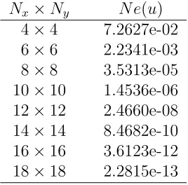
Dirichlet boundary conditions, obtained from (40), are specified on the boundary. The problem domain is embedded in a regular quadrilateral of 2×2 centred at the origin. Figure 3 shows the plot ofu over the extended domain.

There are two versions to be employed here. The first version uses ICS0, ICS1 and ICS2. At the boundary grid-points, only the boundary conditions are imposed. In the second version, ICS0 and ICS2 are employed. This version forces both the boundary conditions and the governing equation to be satisfied at the boundary grid-points. Numerical results show that the two versions yield spectral accuracy and they have similar degrees of accuracy. Unlike the case of rectangular domains

(15)

[25], satisfaction of the governing equation at the boundary grid-points here does not result in a significant improvement in accuracy. Table 2 presents errors Ne(u) obtained by the second version.

4.2 Example 2 (domain with holes)

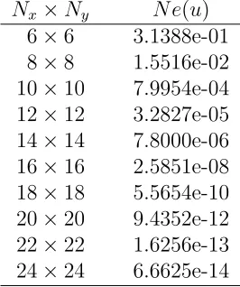
This problem takes the exact solution and driving function as

ue(x, y) = sin(2πx) cosh(2y)−cos(2πx) sinh(2y), (42) b(x, y) = 4(1−π2) [sin(2πx) cosh(2y)−cos(2πx) sinh(2y)]. (43)

A domain with several holes is employed (Figure 4). The domain and the square hole are chosen as [−1,−1]×[1,1] and [1/10,−9/10]×[9/10,−1/10], respectively. The circular hole has its centre at (-1/2,1/2) and a radius of 2/5. Dirichlet boundary conditions, obtained from (42), are specified along the boundaries. Figure 4 also shows the variation of the functionu over this extended domain.

The ICS2 scheme is employed to solve the problem. Results concerning Ne(u) are given in Table 3, which indicate that the approximate solution converges exponen-tially to the exact solution as the grid is refined.

4.3 Example 3 (Neumann boundary condition)

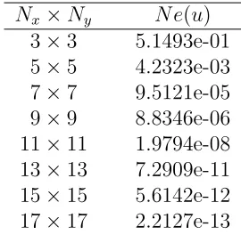
Consider an irregularly shaped domain as shown in Figure 5. The edge CD takes a Neumann boundary condition, while the others are specified with Dirichlet boundary conditions. Positions of points A, B, C, D, E and F are (0,-1), (-1,1), (1,0), (0,1), (-1,1) and (-1,0), respectively. EF is an arc centered at (-1,-1). The exact solution and driving function used here are given below

ue(x, y) = x[sin(2x) cosh(2y)−cos(2x) sinh(2y)], (44) b(x, y) = 4 [cos(2x) cosh(2y) + sin(2x) sinh(2y)]. (45)

The variation of ue over the extended domain defined by [−1,−1]×[1,1] is also shown in Figure 5. Discretizations are carried out using ICS0 and ICS2. The former is applied for lines AB, BC, DE and EF. Table 4 shows that the proposed fictitious-domain technique yields an exponential rate of convergence when the grid is refined.

4.4 Example 4 (domain decomposition)

(16)

whether the rapid convergence of the solution with respect to grid refinement is preserved when the proposed fictitious-domain technique is employed in conjunction with domain decompositions.

Consider a Dirichlet problem with the domain of interest being composed of 2 oc-tagons of unit inradius (Figure 6). The exact solution and driving function are

ue(x, y) = cosπ 2x

sinh(y), (46)

b(x, y) =

1−π

2

cosπ 2x

sinh(y). (47)

The present multi-domain scheme is based on the substructuring technique (cf. [33]). The problem domain is divided into two non-overlapping subdomains (Figure 6). The solution procedure consists of two stages. In the first stage, one deals with the interface solution, while the second stage involves finding the solution of subdomains. Each subdomain is embedded in the reference square domain, and ICS0 and ICS2 are employed to discretize the governing equation. Continuity of the functionuand its normal derivative is imposed pointwise along the interface. Results obtained are displayed in Table 5, showing that the fictitious-multidomain technique also provides a very fast convergence as the grids on subdomains are refined.

4.5 Example 5 (singular solution)

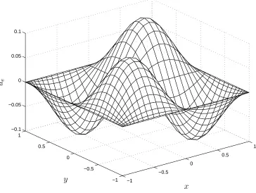
This example is concerned with the case of singular solutions. A non-rectangular domain with curved and straight boundaries is considered here (Figure 7). The curve is an arc having its centre at (-1,-1) and a radius of 2. The present singularity of the solution is due to incompatibility of the differential equation (∇2_u_{= 1) with}

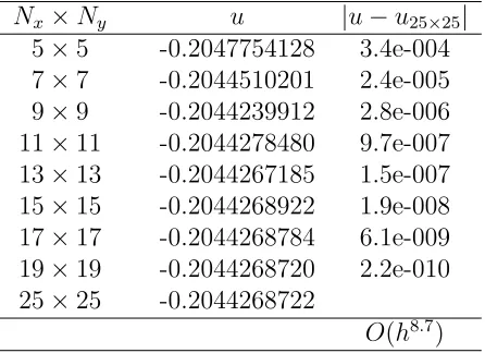
the boundary conditions (u=0) at the lower left corner (mild singularity). The approximate solution u is represented by means of ICS1. Table 6 shows the values of u at point (0,0). Since the exact solution is not known, the values of u obtained with coarse grids are compared with the value ofuwith the fine grid (25×25). Like conventional pseudospectral techniques, in this case (singular solution), the proposed technique is capable of yielding an algebraic convergence rate only. However, it can be seen that the obtained convergence rate is fast, up toO(h8.7_).

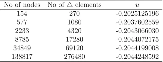
We have also employed a finite-element method (FEM) to solve this problem. The present FEM results (Table 7) were obtained using the PDE tool in MATLAB. To have the solution converged to 5 significant digits, the FEM requires a mesh that is finer than that of 69,120 linear triangular elements and 34,849 nodes. It is noted that the present technique is able to provide a solution with 9 significant digits using a relatively coarse grid of 19×19 (361 nodal points) (CPU time < 1 sec, Pentium 4–2.4GHz, MATLAB environment). Thus, it appears that the proposed technique is more efficient than the FEM. However, for a solution with low regularity (strong singularity), the accuracy of the Chebyshev approximations deteriorates and

(17)

there is no significant advantage over low-order approximation methods. In such a circumstance, a suitable treatment of the singularities is needed in order to obtain a high level of accuracy. This issue has been dealt with and reported in the literature, see, e.g., [14].

5 CONCLUDING REMARKS

This paper reports a new global fictitious-domain/integral-collocation method for the numerical solution of second-order elliptic PDEs in irregularly shaped domains. The construction of the Chebyshev approximations representing the dependent vari-able and its derivatives is based on integration rather than conventional differenti-ation. Information about the actual boundary is taken into account through the transformation of the spectral space into the physical space. Different types of do-mains (simply-connected dodo-mains, multiply-connected dodo-mains and multi-dodo-mains) and of boundary conditions (Dirichlet and Neumann boundary conditions) are con-sidered. Numerical results obtained show that, for smooth (analytic) solutions, the technique yields an exponential rate of convergence as the grid is refined. With this very high order accuracy (comparing with second-order accuracy of the Lagrange-multiplier-based fictitious-domain technique), the present technique is particularly attractive for solving problems where high accuracy is required.

ACKNOWLEDGEMENTS

This work is supported by the Australian Research Council. The authors are grateful to Prof. R.I. Tanner and Prof. X.-J. Fan for fruitful discussions throughout this study.

REFERENCES

1. Glowinski R, Kuznetsov Yu. Distributed Lagrange multipliers based on ficti-tious domain method for second order elliptic problems. Computer Methods

in Applied Mechanics and Engineering 2007; 196: 1498–1506.

2. Young DP, Melvin RG, Bieterman MB, Johnson FT, Samant SS, Bussoletti JE. A locally refined rectangular grid finite element method: Application to computational fluid dynamics and computational physics. Journal of

Compu-tational Physics 1991;92: 1–66.

3. Glowinski R, Pan T-W, Hesla TI, Joseph DD, Priaux J. A fictitious domain approach to the direct numerical simulation of incompressible viscous flow past moving rigid bodies: application to particulate flow. Journal of Computational

Physics 2001; 169: 363–426.

(18)

5. Glowinski R, Pan T-W, Priaux J. A fictitious domain method for Dirichlet problem and applications. Computer Methods in Applied Mechanics and

En-gineering 1994; 111: 283–303.

6. Glowinski R, Pan T-W, Priaux J. A fictitious domain method for external incompressible viscous flow modeled by Navier-Stokes equations. Computer

Methods in Applied Mechanics and Engineering 1994; 112: 133–148.

7. Bertrand F, Tanguy PA, Thibault F. A three-dimensional fictitious domain method for incompressible fluid flow problems. International Journal for

Nu-merical Methods in Fluids 1997; 25: 719–736.

8. Patankar NA, Singh P, Joseph DD, Glowinski R, Pan T-W. A new formulation of the distributed Lagrange multiplier/fictitious domain method for particulate flows. International Journal of Multiphase Flow 2000; 26: 1509–1524.

9. Yu Z, Phan-Thien N, Fan Y, Tanner RI. Viscoelastic mobility problem of a system of particles. Journal of Non-Newtonian Fluid Mechanics 2002; 104: 87–124.

10. Yu Z. A DLM/FD method for fluid/flexible-body interactions. Journal of

Computational Physics 2005; 207: 1–27.

11. Gottlieb D, Orszag SA. Numerical Analysis of Spectral Methods: Theory and

Applications. SIAM: Philadelphia, 1977.

12. Canuto C, Hussaini MY, Quarteroni A, Zang TA. Spectral Methods in Fluid

Dynamics. Springer-Verlag: New York, 1988.

13. Trefethen LN. Spectral Methods in MATLAB. SIAM: Philadelphia, 2000.

14. Peyret R. Spectral Methods for Incompressible Viscous Flow. Springer-Verlag: New York, 2002.

15. Owens RG, Phillips TN. Computational Rheology. Imperial College Press: London, 2002.

16. Orszag SA. Spectral methods for problems in complex geometries. Journal of

Computational Physics 1980; 37: 70–92.

17. Karniadakis GE, Sherwin SJ. Spectral/hp Element Methods for CFD. Oxford University Press: Oxford, 1999.

18. Brebbia CA, Walker S.Boundary Element Techniques in Engineering. Newnes-Butterworths: London, 1980.

19. Mai-Duy N, Tran-Cong T. Approximation of function and its derivatives using radial basis function networks. Applied Mathematical Modelling 2003; 27: 197–220.

(19)

20. Mai-Duy N, Tran-Cong T. Numerical solution of differential equations using multiquadric radial basis function networks. Neural Networks 2001; 14: 185– 199.

21. Kansa EJ, Power H, Fasshauer GE, Ling L. A volumetric integral radial basis function method for time-dependent partial differential equations: I. Formu-lation. Engineering Analysis with Boundary Elements 2004;28: 1191–1206.

22. Madych WR, Nelson SA. Multivariate interpolation and conditionally positive definite functions, II. Mathematics of Computation 1990; 54: 211-230.

23. Mai-Duy N. Solving high order ordinary differential equations with radial basis function networks. International Journal for Numerical Methods in Engineer-ing 2005; 62: 824–852.

24. Mai-Duy N. An effective spectral collocation method for the direct solution of high-order ODEs. Communications in Numerical Methods in Engineering

2006; 22: 627–642.

25. Mai-Duy N, Tanner RI. A spectral collocation method based on integrated Chebyshev polynomials for biharmonic boundary-value problems. Journal of

Computational and Applied Mathematics 2007; 201: 30–47.

26. Mai-Duy N, Tran-Cong T. An efficient domain-decomposition pseudo-spectral method for solving elliptic differential equations. Communications in

Numer-ical Methods in Engineering, in press.

27. Greengard L. Spectral integration and two-point boundary value problems.

SIAM Journal on Numerical Analysis 1991; 28: 1071–1080.

28. Viswanathan RV. Solution of Poisson’s equation by relaxation method–normal gradient specified on curved boundaries. Mathematical Tables and Other Aids

to Computation 1957; 11: 67–78.

29. Thuraisamy V. Approximate solutions for mixed boundary value problems by finite-difference methods. Mathematics of Computation 1969; 23: 373–386.

30. Thuraisamy V. Monotone type discrete analogue for the mixed boundary value problem. Mathematics of Computation 1969; 23: 387–394.

31. Sanmiguel-Rojas E, Ortega-Casanova J, del Pino C, Fernandez-Feria R. A Cartesian grid finite-difference method for 2D incompressible viscous flows in irregular geometries. Journal of Computational Physics 2005; 204: 302–318.

32. Atkinson KE. The numerical evaluation of particular solutions for Poisson’s equation. IMA Journal of Numerical Analysis 1985; 5: 319–338.

33. Smith BF, Bjorstad PE, Gropp WD. Domain Decomposition Parallel

Multi-level Methods for Elliptic Partial Differential Equations. Cambridge University

(20)

[image:20.612.85.559.127.276.2]

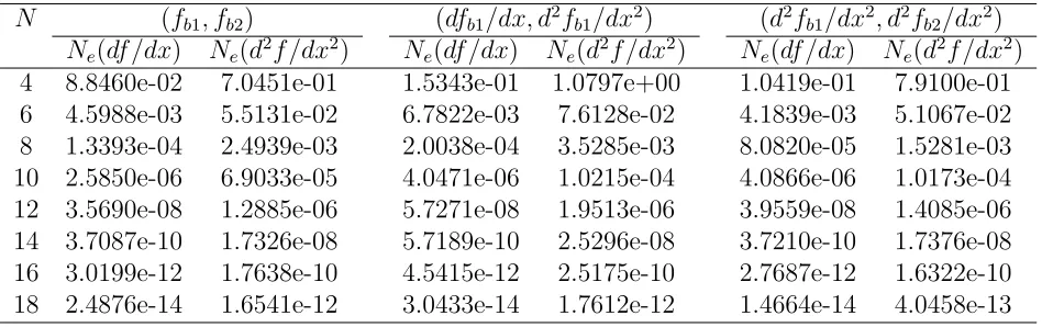
Table 1: f = sin(πx),−1≤x≤1: Relative L2 errors of df /dx and d2f /dx2 by the

integral collocation approach. Apart from nodal function values, extra information given atxb1 =−1/3 and/or xb2 = 1/3, which do not coincide with any grid points,

is also imposed. An exponential rate of convergence is achieved for all cases.

N (fb1, fb2) (dfb1/dx, d2fb1/dx2) (d2fb1/dx2, d2fb2/dx2)

Ne(df /dx) Ne(d2_{f /dx}2₎ _N_e(_{df /dx}₎ _N_e(_d2_{f /dx}2₎ _N_e(_{df /dx}₎ _N_e(_d2_{f /dx}2₎

4 8.8460e-02 7.0451e-01 1.5343e-01 1.0797e+00 1.0419e-01 7.9100e-01

6 4.5988e-03 5.5131e-02 6.7822e-03 7.6128e-02 4.1839e-03 5.1067e-02

8 1.3393e-04 2.4939e-03 2.0038e-04 3.5285e-03 8.0820e-05 1.5281e-03

10 2.5850e-06 6.9033e-05 4.0471e-06 1.0215e-04 4.0866e-06 1.0173e-04

12 3.5690e-08 1.2885e-06 5.7271e-08 1.9513e-06 3.9559e-08 1.4085e-06

14 3.7087e-10 1.7326e-08 5.7189e-10 2.5296e-08 3.7210e-10 1.7376e-08

16 3.0199e-12 1.7638e-10 4.5415e-12 2.5175e-10 2.7687e-12 1.6322e-10

18 2.4876e-14 1.6541e-12 3.0433e-14 1.7612e-12 1.4664e-14 4.0458e-13

(21)

[image:21.612.231.365.87.219.2]

Table 2: Example 1: Relative L2 errors of the solution u. An exponential rate of

convergence is achieved.

Nx×Ny N e(u)

4×4 7.2627e-02

6×6 2.2341e-03

8×8 3.5313e-05

(22)

[image:22.612.231.364.88.247.2]

Nx×Ny N e(u)

6×6 3.1388e-01

8×8 1.5516e-02

10×10 7.9954e-04 12×12 3.2827e-05 14×14 7.8000e-06 16×16 2.5851e-08 18×18 5.5654e-10 20×20 9.4352e-12 22×22 1.6256e-13 24×24 6.6625e-14

(23)

[image:23.612.229.364.85.217.2]

Nx×Ny N e(u)

3×3 5.1493e-01

5×5 4.2323e-03

7×7 9.5121e-05

9×9 8.8346e-06

(24)

[image:24.612.197.399.86.189.2]

Nx×Ny/subdomain N e(u)

3×3 1.4926e-003

5×5 7.7614e-005

7×7 4.0172e-007

9×9 1.6790e-009

11×11 4.5440e-012

13×13 1.1983e-013

(25)

[image:25.612.187.410.116.278.2]

Table 6: Example 5: Computed values of u at point (0,0). For singular problems, the proposed method, like conventional pseudospectral methods, is only capable of yielding an algebraic rate of convergence. The values ofu(0,0) obtained with coarse grids are compared with the value ofu(0,0) with the fine grid (25×25).

Nx×Ny u |u−u25×25|

5×5 -0.2047754128 3.4e-004

7×7 -0.2044510201 2.4e-005

9×9 -0.2044239912 2.8e-006

11×11 -0.2044278480 9.7e-007 13×13 -0.2044267185 1.5e-007 15×15 -0.2044268922 1.9e-008 17×17 -0.2044268784 6.1e-009 19×19 -0.2044268720 2.2e-010 25×25 -0.2044268722

(26)

[image:26.612.162.434.86.190.2]

Table 7: Example 5: Computed values ofuat point (0,0) by FEM. The linear-FEM results are obtained using the PDE toolbox in MATLAB.

No of nodes No of △elements u

154 270 -0.2025125196

577 1080 -0.2037602559

2233 4320 -0.2043066030

8785 17280 -0.2044072175

34849 69120 -0.2044199008

138817 276480 -0.2044248592

(27)

A B C D

E

a a′

b b′

c c′

d d′

[image:27.612.120.474.95.572.2]

e e′

Figure 1: Extended domain. An irregular domain is embedded in a rectangular domain which is then discretized using a tensor product grid. Lines aa′_{, bb}′_{, cc}′_{, dd}′

andee′ _{present typical cases for the approximation of derivatives of the field variable}

(28)

10−2 10−1 100 10−14

10−12 10−10 10−8 10−6 10−4 10−2 100 102

Differential Integral

h Ne

(

d

2 f

/d

x

[image:28.612.110.479.46.341.2]

2 )

Figure 2: f = sin(πx),−1≤x≤1: RelativeL2errors (Ne) ofd2f /dx2. The integral

approximation scheme takes into account not only the nodal function values but also the values of df /dx and d2_{f /dx}2 _at _x _{= 0. Since the discretizations used here are}

chosen such thatx= 0 is a grid point, the integral and differential formulations use the same grids. The former yields a higher level of accuracy than the latter. It is noted thath is the average spacing defined as h= 2/N.

(29)

−1

−0.5

0

0.5

1

−1 −0.5

0 0.5

1 −0.1 −0.05 0 0.05 0.1

x y

[image:29.612.115.479.40.314.2]

ue