Separators in High-Genus Near-Planar Graphs

(1)

Rochester Institute of Technology

RIT Scholar Works

Theses Thesis/Dissertation Collections

12-2016

Separators in High-Genus Near-Planar Graphs

Juraj Culak

[email protected]

Follow this and additional works at:http://scholarworks.rit.edu/theses

Recommended Citation

(2)

APPROVED BY

SUPERVISING COMMITTEE:

Dr. Ivona Bez´akov´a, Supervisor

Dr. Edith Hemaspaandra, Reader

(3)

Separators in High-Genus Near-Planar Graphs

by

Juraj Culak, B.S.

THESIS

Presented to the Faculty of the Golisano College of Computer and Information Sciences

Rochester Institute of Technology in Partial Fulfillment

of the Requirements for the Degree of

Master of Science in Computer Science

Department of Computer Science

Rochester Institute of Technology

(4)

Abstract

Juraj Culak, M.S.

Rochester Institute of Technology, 2016

Supervisor: Dr. Ivona Bez´akov´a

Graph separators are a powerful tool that are motivated by divide and conquer algorithms on graphs. Results have shown the existence of separators

(5)

Chapter 1

Introduction

1.1

Background

Separators in graphs are a valuable tool that can be used to obtain fast algorithms for many graph problems. A separator splits the graph into two unconnected regions of similar size where these regions only share a small boundary region, the separator. Separators can be used in divide and conquer algorithms on graphs. In particular, problems that are suited to divide and conquer solutions are structured such that the problem may be solved recur-sively on smaller subproblems where these solutions are combined over the

boundary region.

To solve a problem by divide and conquer, the original problem can be divided into smaller problems. These subproblems can be solved independently of each other and in a similar manner to the original problem with relatively smaller cost. When dividing the original problem it is necessary to insure that

(8)

are related to each other in the original case in this boundary region.

For graph problems, using a separator is a basic approach to setting up such problems. When a separator is found in a graph, then the graph can be divided into three components. The division yields two roughly equally sized components that do not have any edges between them, while a third relatively small component, the separator, forms the only connection. Thus the problem can be solved recursively on the two separated components and merged using the separator component.

The existence of separators, and efficient algorithms to find them, in specific classes of graphs is useful when designing algorithms for solving more difficult problems. Not all graphs have a proper separator. The complete graph does not have any nontrivial subset of vertices that can be removed that make the graph unconnected, and therefore it is not possible to find a separator.

However when restrictions on the structure of graphs are imposed, sep-arators can be easier to find. For instance a simple cycle can be separated by taking a pair of vertices that have large distance between them as a simple separator. Planar graphs, with their very restricted structure, are a class of

(9)

1.2

Separators

The idea of a vertex separator for a graph is to identify a set of vertices in a graph, that when removed divide the remaining vertices into two balanced unconnected partitions. Informally, given a graphG, the vertex separator is a set of vertices, S, that is a cut set and where the remaining vertices in G\S form two unconnected regions A and B where three main properties hold. The regionsA and B are separated, i.e., there is no edge between the regions. Both regions A and B are not too large relative to the number of vertices in graph G. Finally the size of the separator is small. Furthermore, ideally the separator could be found efficiently.

Definition 1 (Cut Set). Given undirected graph G = (V, E), a cut set is constructed from V by partitioned V into three sets A, B, S, where the sets A

andB are unconnected, i.e., for all verticesu∈A and v ∈B there is no edge e= (u, v) in E. The set S is a cut set.

Definition 2 (Balanced Cut Set). Given undirected graph G with a cut set S that partitions the graph into unconnected partitions A and B, S is said to be

a balanced cut set, with respect to balance parameter a, if |A| ≤ a|V| and

|B| ≤a|V| for a given constant a that is 0< a <1.

Definition 3 (Vertex Separator). A set S of vertices is a vertex separator

for undirected graph G= (V, E) with n vertices, if G be partitioned into three sets A, B, S, the following conditions are satisfied:

(10)

2. (Balanced): the cut set S is balanced with respect to the given balance

constant a,

3. (Small Separator): S has size |S| =f(n), given separator size function f(n).

A class of graphs is said to have a separator with respect toaand f(n) if a vertex separator can be found for every graph in the class. The constanta and functionf are different depending on the specific class of graphs discussed. However, for the separator to have any nontrivial meaning the bound on the size of the separator must be|S|=o(n). Otherwise, the size of the separator would be large relative to the original graph, and therefore would not aid in

divide and conquer techniques. For example, in a grid graph, a separator of O(√n) can be found by taking a single row or column of vertices. ThisO(√n) bound is the also the best bound for the class of planar graphs [1]. In this work the parameters have valuea = 2/3 and f(n) = √n unless otherwise noted.

1.3

Motivation

(11)

1.3.1 Divide and Conquer Techniques

Graph separators can be used as a tool to solve many difficult and specific problems. The main application is in “divide and conquer” problems. Divide and conquer is a technique used to solve computational problems by dividing the problem into smaller problems, applying the solution recursively

to each subproblem, and combining the solutions of the subproblems to get a complete solution to the original problem. This combining stage must do additional work at the boundary between the divided portions to produce the correct solution.

The structure of the partitions formed by the separator is directly able to be exploited by divide and conquer problems [2]. The two partitions A and B are the subproblems that must be solved recursively, and the theorem restricts their size to be smaller and balanced with size up to a|V| for both partitions A, B, while the separator S is the boundary region on which the combination stage occurs, whose size isO(f(n)).

This suggests that the time complexity of the solution can be con-strained, depending on the difficulty of recombining the solution g(n). A recurrence for the time complexity of the solution,T, can be stated:

T(|V|) = T(|A|) +T(|B|) +g(|S|)

Applying the balance constanta, and the separator size function yields:

(12)

A separator size off(n) =√n as in the planar graph class:

T(n) = T(an) +T((1−a)n−O(√n)) +g(O(√n))

Assuming relatively equal partitions, a small separator, and that the combi-nation complexity isO(|S|), i.e.,g(n) =O(n):

T(n) = 2T(n/2) +c√n

The master theorem for the analytic solution to recurrence relations [3] yields:

T(n) = O(n)

In fact as long as the difficulty of the combination stage is not hard, i.e., g(n) =O(nk_{), then for graph classes where a separator can be found and the}

problems can be solved using divide and conquer, a solution can be found in polynomial time.

1.3.2 Additional Separator Uses

(13)

is a new lower time bound ofO(n(logn)3_{) for finding the length of the shortest}

cycle in a planar directed graph that was found using this separator technique [4].

Additionally, separators allow for efficient data representations of graphs [5]. The graph is separated recursively until the number of vertices in each component is small enough to allow a preset number of bits to represent each vertex in the component. This allows the storage for each component inde-pendently to reduce redundant information. Another use of separators has been to provide efficient approximation schemes for combinatorial problems

encoded in graphs [6].

1.3.3 Report Structure

This work examines planar separators and beyond. Chapter One looks at motivations for graph separators and examines divide and conquer tech-niques. Chapter Two looks at planar separators, and the proof of the planar separator theorem in detail. A separator that is also a cycle is described, along with examples of simple planar graph classes. Chapter Three examines

(14)

Chapter 2

Planar Separators

The case of separators for general planar graphs is examined in this section. A proof of the Lipton-Tarjan planar separator theorem is described in detail, and the main components of the proof are examined. Later, examples of planar graphs with simpler separators are examined to illustrate separators.

2.1

Preliminaries

A planar graph is a graph that can be embedded in a plane without any edges crossing each other. Embeddings of planar graphs are not unique, and an embedding can be found for any planar graph in linear time [1]. The pla-nar separator theorem does not require a specific embedding, and a separator

(15)

the existence of a separator that is a simple cycle in planar graphs that are tri-angulated, i.e., every face in the embedding is formed by exactly three edges [8]. The simple structure of this separator allows for easier reasoning when using the separator result to examine more difficult problems. Additionally, it is desirable to find a separator quickly. Lipton and Tarjan showed that planar

separators can be found within linear time [9].

The planar separator theorem uses some graph theoretic terminology. The diameter of a graphGis the maximum distance between any two vertices in the graph. A breadth first search tree of Gis a structure that organizes the

vertices of G. The vertices are organized into a set of levels which partition the vertices of the graph as follows. The first layer L0 is the set containing

just a root vertex v. Each additional layer Li contains vertices which are at

distance i from v. To contract of a set of vertices in G, the set of vertices is removed from the graph, and a new contracted vertexv is added to the graph, along with edges between v and each of the neighbors of vertices in the set of removed vertices.

(16)

2.2

Planar Separator Theorem

The planar separator theorem as presented by Lipton and Tarjan [1] is often used as a basis for separator theorems for more complicated classes, and an understanding of it is useful for separator results in non-planar graph classes. Specific values are assigned to the constanta= 2/3 on the size of the partitions and the functionf(n) =√n constraining the size of the separator. The planar separator theorem can be extended to weighted graphs. Also, Lipton and Tarjan give an O(n) algorithm for producing the separator.

Theorem 1 (Lipton-Tarjan Planar Separator Theorem [1]). Let G be any n-vertex planar undirected graph. The vertices of G can be partitioned into

three sets A, B, S, such that no edge joins a vertex in A with a vertex in B,

neither A nor B contains more than 2n/3 vertices, and S contains no more

than4√2n+ 6 vertices.

2.2.1 Proof of the Planar Separator Theorem [1]

(17)

2.2.1.1 Diameter Reduction

The diameter of the graph, G, is reduced as follows. Construct a breadth first search tree of G from an arbitrary root vertex, v. The ver-tices in the graph are divided into different levels of the search tree. Each level is labeled Li where i is the distance to the starting vertex. An extra level is

created asLd+1 and contains no vertices. Note that any level Li is a cut set,

since each vertex in levels closer to the root than i is not directly adjacent to vertices that are further from the root than i. However this cut set may be neither balanced nor small. The desired separator should be a cut set that is both small and balanced. If any level is both balanced and small then this level in the tree forms the separator.

There is some median level, Lm, where the number of vertices in the

levels closer to the root vertex than the median level is less thatn/2, and the same holds for levels further from the root. There is some level Lα closer to

the root than Lm which has less than

√

n vertices. Similarly there is a level Lβ further from the root with less than

√

n vertices. LevelsLα and Lβ are the

closest levels to the Lm of those that satisfy the small number of vertices. The

median level must be at least distance 1 from the root, and therefore the root level with one vertex may be Lα since |L0| = 1 ≤

√

n. Similarly, the empty level has 0≤√nvertices, and may be Lβ if there is no level closer to the root

vertex with the appropriate size.

We claim the distance between the two levels Lα above andLβ below is

(18)

between Lα and Lβ has at least

√

n vertices, otherwise that level would have been chosen as Lα orLβ. The number of vertices in the levels fromLα toLβ is

β

P

j=α

|Lj|, and note the number of vertices inG isn. So let k be the number of

levels Lj between Lα and Lβ, then n≥ β

P

j=α

|Lj|=avg(Lj)·k ≥min(Lj)·k ≥

√

n·k. Thus n≥k√nand k ≤√n. Thus there are at most √n levels with at least√nvertices since√n·√n≤n. Thus we have a small, i.e.,O(√n) cut set that is the union of levelsLαand Lβ, where the middle levelsLα+1∪. . .∪Lβ−1

containingLm are one vertex set A, and L0∪. . .∪Lα−1∪Lβ+1∪. . .∪Ld the

second vertex setB. However this cut set, though it satisfies the small size and separation conditions for a separator, it may not produce balanced separated setsAandB. Again, if the cut set produced does satisfy the balanced property then this can be the separator that is the result of the construction.

Otherwise the diameter of the graph must be reduced, so that the fundamental cycle lemma can be applied to produce a small separator. The levels between Lα and Lβ contain more than 2/3 of the total vertices, since

otherwise the cut set would be balanced. The vertices inLαand all levels closer

to the root are contracted to a single vertex. This contracted vertex represents a small set, of size no more thann/3, and similarly the vertices further from the root thanLβ have size at mostn/3 in the original graph. Notenis the number

of vertices in the original graph G. Thus we can construct a new graph G∗ by taking the contracted vertex along with the vertices in the middle region, while discarding the vertices in level Lβ and those vertices further from the

(19)

from the new contracted root vertex to the farthest vertex is at most 1 +√n. The breadth first search spanning tree now has diameter of at most 2 + 2√n.

2.2.1.2 Fundamental Cycle Lemma

Lemma 1 (Fundamental Cycle Lemma [1]). For any planar graph H with

diameter d, H can be partitioned into A, B, S where A and B are balanced

(|A|,|B|<2/3|V(H)|), and|S| ≤2d+ 1.

2.2.1.3 Proof of Fundamental Cycle Lemma [10]

The lemma states that a planar graph that is of diameter d has a balanced cut set with size at most 2d+ 1. Given a graph and an embedding, a triangulated graph is constructed by adding edges to the original graph connecting vertices until each face has exactly three boundary edges, while

maintaining planarity. A cut set can be constructed in the triangulated graph and its planar embedding, and examining the spanning tree in the graph. The depth of the tree is bounded by the diameter. This fundamental cycle cut set is a simple cycle in the triangulated graph that forms a vertex separator.

(20)

y

z

x _e

[image:20.612.237.393.115.201.2]

g f

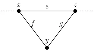
Figure 2.1: The triangulated face containing e, that forms a cycle.

path plus the single edge, therefore|C| ≤ 2d+ 1. The Jordan curve theorem states that a closed curve in a plane divides the plane into an interior and

an exterior region which are unconnected [10]. This cycle follows the Jordan Curve Theorem and it divides theH into two unconnected regions.

We will now show that there is at least one non-tree edgee, that when added to the tree forms a cycle which makes the number of vertices on the in-terior and the exin-terior regions balanced so both have size less than 2/3|V(H)|. Consider the edge that is not a member of the tree, that when added to the tree to form a cycle C, minimizes the maximum size of the outside or in-side regions, where ties are broken by minimizing the number of faces on the maximum size side. We claim e forms a cycle that balances the inside and outside.

(21)

C to be larger than that outside the cycle, otherwise the same analysis can be performed where the emphasis is on placing vertices in the exterior rather than the interior. Since e is a non-tree edge, thenf and g can be both on the cycle, only one is on the cycle, or neither are on the cycle.

1. In the case where both f and g are on the cycle, then the cycle must be (e, f, g), as in Figure 2.1. This cannot be the case since then there are no

vertices inside the cycle, therefore this would be imbalanced. A better edge could have been chosen, forming a contradiction on the choice ofe.

2. If one edgef is on the cycle, then the edgeg is in the larger region inside the cycle, and the cycle contains eandf. In this caseg would have been chosen as the non-tree edge, since that would form a cycle where one additional vertex x would be contained in the originally smaller region, making it now more balanced.

3. Otherwise neither f nor g are on the cycle. Now, there are cases on whether f and g are tree edges: edges f and g are both tree edges, one

is a tree edge, or neither is in the spanning tree.

(a) If both are tree edges, then the tree edges that form the cycle with e, would also form a cycle with f and g, and the tree would contain a cycle, a contradiction.

(b) Suppose neither f nor g are on the cycle and one edge, f is a tree

(22)

edge g as the best non tree edge would return the same number of vertices in the interior and exterior as before, however with one face less in the larger region, contradicting the choice of e.

(c) Next suppose neitherf nor g are on the cycle, and neither is a tree edge. The vertex y, betweenf and g must be connected to an edge on the spanning tree that is not on the cycle. In this case a new cycle could be drawn that uses vertices from the original cycle plus f or g and the branch of the tree that goes to y. This new cycle divides the interior region of the graph that had size larger that 2|V(H)|/3, making a new more balanced division. Therefore this edge would have been chosen originally.

Each possible case considered yields a contradiction, therefore the choice of e must yield a balanced separator. This separator has size |S| ≤2d+ 1.

2.2.1.4 Producing the Separator

The graphG0constructed fromGby contracting the vertices above and including Lα into a single vertex, and discarding those below and including

Lβ, has diameter d≤ 2

√

n+ 2. Therefore by applying the fundamental cycle lemma we can construct a cycle C in the triangulated and contracted graph with size |C| ≤ 2d+ 1≤ 2√n+ 3 = O(√n), that separates G0 in a balanced way. Now the original graph that is triangulated has a simple cycle located within the layers above Lβ, that separates it into two balanced interior and

(23)

regions are still separated, since removing edges does not connect components. Additionally the regions above Lα and below Lβ are small compared to the

size of the original graph. The separated setsA and B are formed from these disjoint sets, while the separator is constructed fromLα,Lβ, andC. Now since

the condensed graph has diameter 2√n+ 2, we have an O(√n) separator in that graph. A proper balanced and small separator in the original graph can be constructed from the cycle separator and the two layersLα and Lβ in the

original graph, by carefully examining the sizes of all the components.

2.3

Cycle Separator

The separator that the Lipton-Tarjan Planar Separator Theorem yields does not give any structure beyond separating the graph. The vertices that form the separator may be unconnected and additionally vertices contained in each partitions may also be unconnected. If the separator had a guaran-teed simple structure, that allowed easier understanding of how the graph was divided, then the graph and its separation may be better used.

(24)

2.3.1 Construction Sketch [8]

The construction of the simple cycle separator follows a similar idea as the Lipton-Tarjan planar separator construction, however looking at dual graphH of an original triangulated graph G.

The breadth first search tree is constructed in the dual graph,H, with the search starting at a vertex inH, corresponding to a face inG. At the first step, the starting face corresponds to three edges that form a simple cycle. Consider adding vertices in the dual to a set, corresponding to adding faces in the original. If there is an edge in the dual, i.e., the faces are adjacent,

then the union of the faces forms a new group of vertices that have a simple cycle exterior. So a set of vertices in the dual graph corresponds to faces in the original that are surrounded by a set of disjoint simple cycles, where the exterior of each cycle is also disjoint.

The boundary of the exterior faces is a simple cycle in the original

(25)

2.4

Simple Planar Classes

2.4.1 Binary Trees

A simple graph class with an easily found separator is the class of binary trees. These graphs have significant structure that can be exploited. They are trees and therefore do not contain cycles, and every vertex is connected to at most one parent vertex and at most two child vertices. A binary tree can be separated into two partitions, each with size less than 2n/3 with the removal of a single vertex. Since removing any nonleaf vertex from a tree results in unconnected components, a separator can be easily found. The ideal vertex can be found by traversing the tree from the root, always choosing the

child that produces a more balanced partition until a proper 2n/3 partition is found. When this vertex is removed then the tree becomes separated with the partitions balanced, i.e., each set of vertices that remains in the graph after the separator is removed has size 2|V(G)|/3. Thus binary trees have a size 1 separator.

2.4.2 Four-Connected Grid Graphs

Four-connected rectangular grid graphs are an example of a planar

(26)

[image:26.612.201.430.119.239.2]

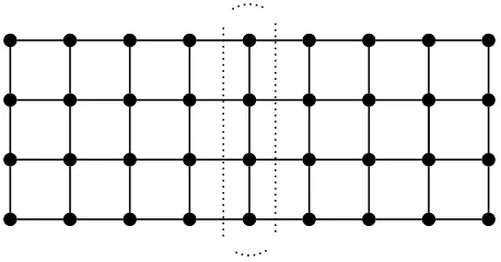
Figure 2.2: A four-connected grid graph, with a separator outlined. Notice when the vertices in the separator are removed from the graph, then the re-maining graph is partitioned into two unconnected sets.

distance 1 in the coordinate system. Since there are no long distance connec-tions, the distance between any pair of vertices increases by at most 2 if any edge is removed.

(27)

Chapter 3

Separators in Other Graph Classes

This section of this work notes the main previous work on graph separa-tors in non-planar graph classes. Then this work investigates the class of high genus non-planar graphs as an interesting graph class to consider for a separa-tor result. The related graph classes of non-planar grid graphs, face-crossing planar graphs, planar overlays, and restricted distance graphs are defined and

examined. Extensions to the planar separator theorem, and its components, are then investigated.

3.1

Previous Work on Non-Planar Classes

The case of planar graphs is a very restricted case, where the graph

has a specific structure. As the structure of the graph becomes more gener-alized, it may no longer be possible to find a separator. For example, in the complete graph there is no set of vertices which when removed leave uncon-nected regions of the graph. There has been work showing that separators can be found efficiently in classes of graphs that are non-planar and have more general structure.

(28)

or loops extending out of the surface that allow curves to cross past other curves without intersecting. When a graph can be embedded in a surface of genus g without any edges crossing, then a separator can be found where

|S| = O((gn)1/2_{) [11]. Consequently graphs of bounded genus, i.e., graphs}

where the genusg is bounded by a constant, g =O(1) even as the size of the

graph is not bounded, have separators where|S|=O(n1/2) [11].

Graphs of bounded genus are a subclass of minor-free graphs, another class of graphs with a restriction on structure. This class is defined using graph minors. A graph minor is a graph that can be formed from the original

graph by deleting edges and contracting vertices. Graph classes that disallow specific minors to be formed from members of the class are known as graphs excluding a fixed minor [12]. For example planar graphs can be defined as the class of graphs that exclude the minors K5, the complete graph with five

vertices, and K3,3, the complete bipartite graph on 3 + 3 vertices. Separator

theorems also exist for classes of graphs that exclude a fixed minor [13].

3.2

Graph Classes to Consider

When graphs are no longer planar, the structure that allowed the con-struction of a separator may not be there, however imposing other structure may allow a separator to be found. In particular when the class is based on modification of a planar graph, i.e., adding crossing edges, then the planar separator for the underlying graph may suggest the construction of the new

(29)

A class of graphs with interesting structure is high-genus near-planar graphs. These graphs have a high genus, where the number of crossings would beω(1), i.e., not bounded by a constant. Additionally, edge crossings would be present in multiple locations of the graph and thus would not be able to take advantage of constant number of topological handles or connections. Therefore

these graphs are not able to be embedded in a surface of constant genus, so the genus of the graph would be not constant, i.e., ω(1), and clearly would not be planar. The near-planarity property of the graph would restrict the graph minimize non-planar crossing and provide structure that would allow an approach to tackling the separator theorem in this more general case. Edge crossings in near-planar graphs are limited so that the non-planar properties of the graph are restricted to local regions. To ensure this the crossed edges must be local to each other, i.e., the distance between the endpoints of crossed

edge pairs is bounded by a constant. Additionally, this class of graphs does not necessarily have an excluded fixed minor. In the general case of high-genus near-planar graphs, when attempting to contract vertices, the diagonal connections can be used to provide links that allow minors to be constructed. Therefore, these graphs cannot be characterized by the previous results about separators [11] [13].

(30)

other edge but the graph has genus where the number of crossings grows with the size of the graph and is not bounded by a constant, since multiple edges cannot be embedded in the handle portion of the surface. Further, the edges that cross are local relative to each other. There is distance 1 between the two crossing edges. Some additional classes of graphs including extended

non-planar grid, face-crossings, non-planar overlays, restricted distance crossings are examined as candidates for extended separator results.

3.3

Non-Planar Grid Graphs

Grid graphs are used in image applications. The vertices represent

pixels, and edge weights can encode pixel level information such as color dif-ferences between pixels. For example grid graphs are used as the basis for encoding images for image segmentation algorithms that use maximum flow algorithms [14]. Increasing the connectedness of a grid representing the im-age allows for local information to be shared at a longer scale, but makes the graphs non-planar.

When the graph has higher connectedness than the four-connected case, then it becomes non-planar, and has high genus, making this an interesting class of graphs to examine. This class of graphs has a useful structure. First, crossing edges are close to each other. In the case of distance-d connected grid graphs, described in section 3.3.2, edges exist between vertices that are at distance d from each other when drawn in an integer grid. This limits the

(31)

[image:31.612.193.441.116.262.2]

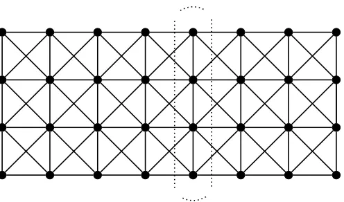
Figure 3.1: An eight-connected grid graph, with a separator outlined.

vertices. Additionally when embedded in a plane grid graphs have clear rows and columns that are intuitive starting points for a separator.

3.3.1 Eight-Connected Grid Graphs

The rectangular eight-connected grid graph is a non-planar high genus graph that also has a very defined structure, shown in Figure 3.1. In these graphs each vertex is connected to its eight nearest neighbors when drawn

(32)

considering a non-planar embedding of the eight-connected grid. Multiple edges cannot be embedded in a handle, since the pairs of edges that cross are not local to other pairs of crossing edges. Further, the edges that cross are local relative to each other. There is distance 1 between the two crossing edges.

Remark 1. The eight-connected grid graph has a separator of size O(√n).

Examining the structure of eight-connected grid graphs informs the size of the separator. The structure in this case of non-planar high genus graphs is its ability to be drawn in a grid like the four-connected grid. The crossings introduced by the eight-connected property only connect across faces that

(33)

3.3.2 Distance-d Connected Grid Graphs

The idea of connected grid graphs can be extended so that every vertex has additional edges connecting it to other close vertices. The notion of close or local vertices can be described by using a distance metricD() in the original unconnected two dimensional grid of vertices. In a distance-d connected grid

graph, there exist an edgee= (u, v) between verticesuandv whereD(u, v)≤

d. The distance between connected vertices and their arrangement in a grid ensures that the crossings occur locally. The specific metric D used changes which vertices are connected. For example with distance d = 2, with the euclidean metric D((x1, y1),(x2, y2)) =

p

(x1−x2)2+ (y1−y2)2, a vertex is

connected to twelve neighbors, the eight nearest neighbors in addition to the four vertices that are at distance two along the axes. While with d = 2 and the maximum metricD((x1, y1),(x2, y2)) =max(|x1−x2|,|y1−y2|), a vertex

is connected to the 24 nearest neighbors that are arranged in a square pattern.

Definition 4(Distance-dConnected Grid Graph). A distance-d connected

grid graph Gwith respect to distance metric D is a graph where the vertices

are arranged in a rectangular a × b integer grid, with the following edges. The vertex u is represented as u = (iu, ju) where iu ∈ [1, . . . , a], and ju ∈

[1, . . . , b] are the indices of the vertex in the grid. Given distance metric D where D(u, v) =D((iu, ju),(iv, jv)), there is an edge between a pair of vertices

(34)

3.3.2.1 A Separator in Distance-d Connected Grid Graphs

Consider using the maximum distance metric. At distance d > 1 each vertex is connected to its d2 ₋_{1 nearest neighbors, and every edge crosses}

multiple other edges and the genus of the graph is nonconstant. When the distanced > 1, then a row no longer yields a cut set. However a cut set can

still be constructed by taking a row that would separate the four-connected graph, and taking the union of thedadjacent rows in the distance-dconnected graph. This would separate the graph in a balanced way since the underlying grid would be separated by the original row, and any vertex that is local to that row would have been added to the cut set. This ensures that any edge that originates in one partition of the graph terminates in the separator and thus the partitions are unconnected. The original separator in the four-connected grid has O(√n) and the new separator has size O((2d+ 1)√n) = O(d√n), and d is constant for each case of graph.

Consider a rectangular distance-d connected grid graph G with size

|G|=n, and its embedding in a plane. The graph embedding can be arranged as a p×q grid of vertices, where pq = n. Label each vertex ui,j based on its

location in the grid where 1≤i≤pand 1≤j ≤q. A vertexui,j is connected

to its nearest neighborsui+x,j+y where−d≤x≤dand−d≤y ≤d, using the

maximum distance metric.

Without loss of generality assumep≤q.

(35)

and 1≤k ≤p is a balanced small separator S.

Proof

A proper separator separates the partitions, has partitions that are balanced, and the separator is of small size.

Separated

Claim:

S separates the sets A = {uij | 1 ≤ i ≤ p and 1 ≤ j ≤ m−d} and

B ={uij | 1≤i≤pand m+d≤j ≤q} into two unconnected partitions.

Proof of claim:

NoteA∩B = A∩S =S∩B =∅. Consider any vertex ui0_,j0 ∈ A. If

j < m−2d, then clearly all its neighbors are also within A. Ifm−2d≤j ≤

m−d, then the neighbors above, below, and to the left are clearly within A. The neighbors to the right of ui0_,j for any i0 and j ≥ m−d are the vertices

ui0₊_x,j₊_y. Given that the graph is distance-d, −d ≤ x ≤ d and −d ≤ y ≤ d.

Thusj+x≤m−d+x≤m−d+d≤m. The value ofi0 does not influence the set that ui0_,j is found in. Since all the j coefficients in set B are in the range

j ≥m+d, then ui0_,j must be located in S∪A. Thus all neighbors of u ∈A

(36)

Balanced

Claim:

|A| ≤2n/3 and|B| ≤2n/3 Proof of claim:

The set A is a rectangular grid. Therefore |A| = p(m −d); similarly

|B| = p(j −(m +d)). The total number of vertices is n = pq. Therefore

|A| = p(m−d) = p(bq/2c −d) ≤ p(q/2−d) ≤ pq/2 ≤ n/2 ≤ 2n/3. And,

|B|=p(q−(m+d)) =p(bq/2c)≤p(q−d)/2≤pq/2≤2n/3. And therefore the cut set is balanced.

Small

Claim:

|S|=O(√n) Proof of claim:

The separator S contains all uk,m where 1 ≤ k ≤ p and bq/2c −d ≤

m≤ bq/2c+d. The size of this set isp(bq/2c+d)−p(bq/2c −d) = p(2d+ 1). Since p ≤ q, n = pq ≤ qq, therefore √n ≤ q. Therefore, |S| = p(2d+ 1) = (2d+ 1)n/q ≤(2d+ 1)n/(√n)≤(2d+ 1)√n, and |S|=O(√n). Thus S is a small cut set.

(37)

Corollary 1. The eight-connected grid graph has a separator of size O(√n).

Proof of Remark 1 and Corollary 1

Consider the distance metricD((i1, j1),(i2, j2)) =max(|i1−i2|,|j1−j2|)

with distance d = 1. The graph G with n vertices generated by this is the eight-connected grid graph. Using Lemma 2, this graph has a proper separator of size O(√n).

3.3.3 Multidimensional Grid Graphs

Multidimensional grid graphs are constructed using equally spaced D -dimensional lattice points as vertices and then connecting to the nearest 2D neighbors. The edges e = (u, v) in the graph are as follows, a vertex is la-beled as u : (d1, . . . , dD) where the di is its coordinate in the grid along a

dimension, a connected neighbor has labeling v : (d1, . . . , di+1, . . . , dD) orv :

(d1, . . . , di−1, . . . , dD) for any i, i.e, exactly one index differs by one.

Remark 2. For a multidimensional grid graph G with dimensionality D, a

separator of size O(n(D−1)/D) can be found by taking all the vertices in a D -hyper-plane.

(38)

hD−1_{. Thus the size of the cut set is} _hD−1 ₌ _n(D−1)/D_{, and the cut set is a}

separator.

These graphs can be expanded to be distance-dconnectedD-dimensional grid graphs. In this case the hyper-plane of vertices can be combined with the dadjacent planes to ensure that the remaining partitions do not have an edge connecting them, forming a separator.

3.4

Face-Crossing Non-Planar Graphs

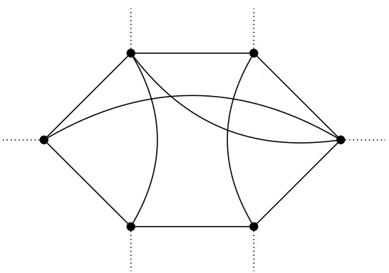
An extension of planar graphs to non-planar, high genus graphs is to consider restrictions on crossings. One such restriction is to allow crossing in the faces of an embedding of a planar graph, as seen in Figure 3.2. The genus of such a graph is non constant and bounded by the size of the largest face F, and the number of faces NF. The genus within the face is O(|F|2),

since there the number of crossing edges increases with the number of pairs of vertices on the graph. The total genus of the graph is O(|F|2_N

F) These

graphs are near-planar since all the crossings take place within original faces, and therefore are localized.

Definition 5(Face-crossing graph). Given a non-planar graph Gand its em-bedding, a face-crossing graph G0 is constructed by adding edges that

con-nect vertices on each face of G.

Remark 3. Face-crossing graphs have a cut set of size O(|F|2_N

F

√

n)

(39)

[image:39.612.180.453.119.311.2]

Figure 3.2: A face-crossing graph. The only crossings are located in faces of a planar base graph.

the structure of the graph. There are no crossings between the original planar faces. The separator for the underlying planar graph would be found using the techniques from the Planar Separator Theorem.

This planar separator could easily be extended to separate the new non-planar graph. For every face that contains vertices that are in the separator of the underlying planar graph, its vertices are added to the cut set. Any edge in the graph now is either in one of the partitions, or has at least one vertex in the separator as required by the separator in the underlying planar graph. Or any new edge has at least one vertex on a face that has been added to the separator. This new cut set has size O(|F|2_N

F

√

n). This may not be a small separator since the size of the face F may be large. However if the

(40)

3.5

Planar Overlays

Planar overlays can be used to construct near-planar graphs. A planar graphG and an embedding is taken as the base of the construction, and then another planar graph H is overlayed on the base. The vertices in the overlay correspond to vertices in the base graph, and the edges from the overlay are added to the base graph. Adding an overlay may make the graph no longer planar.

A separator can be constructed in an overlayed planar graph. The planar separator theorem yields a separator S in the base graph G. The planar separator can be extended by adding vertices from any connection that would have been created by the overlay can be added to the separator. If the

overlay adds only a constant number of edges then |S0|= O(√n). Otherwise the separator would grow too large.

Some restrictions on overlays may allow a separator to be found. The overlay can be restricted to add a limited number of edges at any distance to the original graph. Another restriction could be only on short distance

(41)

3.6

Restricted Crossing Distance Graphs

A class of near-planar high genus graphs that is not constructed from planar graphs but is interesting to consider in relation to separators is the class of restricted crossing distance graphs. In this class of graphs, the distance in the graph between any of the four vertices contained by a crossing pair of edges is bounded by a constantd, when either of the crossing edges is removed. This class of graphs is similar to the distance-d grid graphs, but the vertices are not

restricted to the grid structure. The limited distance forces any crossing to be local, and the crossing edges do not bridge between possible distant partitions.

Definition 6 (Restricted Crossing Distance Graph). Arestricted crossing

distance graph Gis a graph where the following property holds for a constant

d: given a pair of edges e = (u1, v1), f = (u2, v2) that cross, in the graph G0

with the edge e removed, the distance from u1 tov1 is at mostd, and similarly

with the edgef removed, the distance from u2 to v2 is at most d.

If a separator for this class could be found for some planar underlying graph, the separator in this class of graphs would be constructed as a multiple layer separator. The separator could be extended by d vertices near each crossing edge increasing the size toO(hd√_n_{), where}_h_{is the maximum degree}

in the graph.

Remark 4. The graph class of restricted crossing distance does not have a

(42)

This class of graphs has special cases that must be considered. Every vertex on an edge that crosses is only at distance 1 from any other vertex in the complete graph, even when any crossing edge is removed. Consider the complete graphKn. This graph satisfies the conditions of restricted crossing

distance. However, no amount of vertices can be removed from a complete

graph to form two unconnected components. Therefore the complete graph does not have any cut set or separator. It is clear that only restricting the distance between crossing edges is not sufficient to have a proper separator.

3.7

Towards Extending the Planar Separator Theorem

Proof

For these extended high-genus near-planar graph classes, a proof ap-proach similar to the planar separator theorem would be a potential apap-proach to have a separator result for these classes. The non-planar portions of the graph that cross are localized. Therefore the dependence of the proof on the local details of planarity can be reworked taking into account the local non-planarity. The components of the proof that depend on planarity will be attempted using the intuition from the locality of the non-planar portions of the graph.

The main components of the planar separator theorem proof are the breadth first search tree construction, and the fundamental cycle lemma, which uses the planarity of the graph allowing use of the Jordan Curve Theorem.

(43)

chosen. In addition, weaker bounds on the size of the separator could be used to facilitate results.

3.7.1 Breadth First Search Tree Diameter Reduction

In the non-planar case, the layered breadth first search tree can be

constructed in a similar manner as the planar case. If a cycle lemma is able to be applied to the tree without much additional modification, a similar approach as the planar proof would yield a separator. However if any crossing edges bypass the separator, the separator produced from the tree would need to contain multiple layers of vertices.

3.7.2 Fundamental Cycle Lemma

A fundamental cycle lemma for high-genus near-planar graphs would

state for a graphGin the class that has specific structure, thatGcan be parti-tioned intoA,B and the separatorS, where the separator has a bounded size. The structure in the planar case that determined the size of the separator was a spanning tree of depthd. Additionally, the case analysis in the fundamental cycle lemma depends on a triangulation of the original graph, and a examining the case of non-planar graph may allow a similar case analysis [15].

(44)

if the edge crosses the tree, a case analysis could be performed to examine the effects on the separator and additional edges added to it.

If the spanning treeT were crossing in the embedding of G, then there are two possible approaches. The tree T could be modified to get a possibly non crossing spanning tree by swapping edges [16]. Otherwise, the entire faces that contain crossing edges from T could be added to the separator. This approach would need to be limited to non-planar graphs with limited crossing distance, otherwise too many vertices would need to be added to the separator. Only O(√n) vertices could be added. Additionally, the faces added can be contracted to single vertex so a new spanning tree is constructed. The case analysis for adding an edge to make a cycle must take into account the faces added.

3.7.3 Jordan Curve Theorem

Planarity allows the use of the Jordan curve theorem, whereby a closed curve divides a plane into the interior and exterior. In the near-planar case, a connected “dividing” set of vertices can be used to replace the curve, when the

(45)

Chapter 4

Conclusion

This work examined separators in planar graphs and high genus near-planar graphs. Non-near-planar graph classed including multiple non-near-planar grids, face-crossings, planar overlays, and restricted distance crossings were exam-ined as candidates for extended separator results. Each of these graph classes included restrictions on the structure of the graph to allow for the existence

of a separator.

These grid graphs, including 8-connected,d-distance crossings, and D -dimensional, all had very restricted structure. In these graphs a simple sep-arator could be found by taking a set of vertices from a division along the

grid structure and extending the width of the vertex set to encompass the possibility of crossing edges.

Meanwhile in graph classes that extend planar graphs, including pla-nar overlays and face-crossings graphs, a separator can be constructed from the underlying planar separator, but with the addition of extra vertices that

(46)

(47)

Chapter 5

Future Work

The graph classes examined in this work were either too structured and had simple separators, or were not structured enough to yield a separator. Some classes lacked the structure to guarantee a separator or to provide size bounds.

The initial goal with future work is to identify the most interesting class of high genus near-planar graphs, where a proper separator can still be found. The examination of the uses of separator problems or applied graph problems, may instruct the properties of graphs that are useful to investigate. If a general graph class is identified as interesting, then the details of restrictions and graph

properties can be examined with respect to the proof of the separator theorem.

Proving a separator theorem is the primary goal for future work. The investigation of a proof for a separator theorem for a class of graphs informs the restrictions necessary. This work outlines some possible approaches to the proof. In general the planar separator theorem gives a useful framework for

(48)

graph must be examined for its ability to allow an arbitrary separator to be found. The structure of the graph class may need to be changed, in addition to relaxing the desiredO(√n) bound on the size of the separator. The size bound on the separator is likely to depend on a parameter related to the distance in the graph that the crossing edges span.

Another area to explore is divide and conquer problems on graphs. The graph separator is motivated by these problems, so investigating which problems benefit would motivate graph classes to examine. Ideally divide and conquer problems that currently only have solutions in planar cases but have

non-planar variants would benefit from high genus near-planar graphs. Some such problems may be found in image analysis.

Given a separator theorem result, the final step would be to explore an efficient algorithm to generate the separator. In the planar case, the separator can be found in linear time. Additionally, one can implement the algorithm,

(49)

Bibliography

[1] Lipton, R., and Tarjan R. A separator theorem for planar graphs. SIAM Journal on Applied Mathematics 36, 2 (1979), 177-189.

[2] Lipton, R., and Tarjan R. Applications of a Planar Separtor Theo-rem. SIAM Journal on Computing 9, 3 (1980), 615–627.

[3] Cormen, T., Leiserson, C.E., Rivest, R.L., and Stein, C. In-troduction to Algorithms, Third Edition. MIT Press and McGrawHill (2009).

[4] Wulff-Nilsen, C. Girth of a planar digraph with real edge weights in O(n(logn)3) time. arXiv:0908.0697.

[5] Blandford, D., Blelloch, G., Kash, I. Compact representations of separable graphs. Proc. 14th ACM-SIAM Symposium on Discrete Algorithms (2003), 679–688.

[6] Hunt., H, Marathe, M., Radhakrishnan, V., Ravi, S.S., Rosenkrantz,

D.J., and Stearns, R.E. Parallel Approximation Schemes for a Class of Planar and Near Planar Combinatorial Optimization Problems Infor-mation and Computation 173, (2002) 40-63.

(50)

[8] Miller, G. Finding small simple cycle separators for 2-connected planar graphs. Journal of Computer and System Sciences 32, 3 (1986), 265-279.

[9] Holzer, M., Prasinos, G., Schulz, F., Wagner, D. and

Zaro-liagis, C. Engineering planar separator algorithms. ESA 2005: 13th Annual European Symposium, Proc., (2005) 628–639.

[10] _{Klein, P. and Mozes, S.} Optimization Algorithms for Planar Graphs.

<http://planarity.org/>

[11] Gilbert, J., Hutchinson, J., and Tarjan, R. A separator theorem for graphs of bounded genus. Journal of Algorithms 5, 3 (1984), 391-407.

[12] Demaine, E., Mozes, S., Sommer, C., and Tazari, S. Algorithms for Planar Graphs and Beyond. MIT, 6.889 (Fall 2011).

[13] Reed, B. and Wood, D. A linear-time algorithm to find a separator in a graph excluding a minor. ACM Transactions on Algorithms 5, 4 (2009) 1-16

[14] _{Boykov, Y., and Kolmogorov, V.} An experimental comparison of min-cut/max-flow algorithms for energy minimization in vision. IEEE

Transactionson Pattern Analysis and Machine Intelligence 26, 9 (2004), 11241137.

[15] Aichholzer, O., Cabello, S., Fabila-Monroy, R., Flores-Penaloza

(51)

Edge-Removal and Non-Crossing Configurations in Geometric Graphs. Dis-crete Mathematics and Theoretical Computer Science 12, 1 (2010) 119– 122.

[16] _{Aichholzer, O., Aurenhammer, F., Hurtado, F.} Edge Operations on Non-Crossing Spanning Trees. In Proc. 16th European Workshop on

Theses

Thesis/Dissertation Collections

Separators in High-Genus Near-Planar Graphs

Rochester Institute of Technology

APPROVED BY

Separators in High-Genus Near-Planar Graphs

THESIS

Rochester Institute of Technology

Table of Contents

Chapter 1

Separators

Motivation

Chapter 2

Planar Separator Theorem

Cycle Separator

Simple Planar Classes

Chapter 3

Previous Work on Non-Planar Classes

Graph Classes to Consider

Non-Planar Grid Graphs

Face-Crossing Non-Planar Graphs

Planar Overlays

Restricted Crossing Distance Graphs

Towards Extending the Planar Separator Theorem

Chapter 4

Chapter 5

Bibliography