A finite difference routine for the solution of transient one dimensional heat conduction problems with curvature and varying thermal properties

Purpose

The Faculty of Engineering & Surveying Technical Reports serve as a mechanism for disseminating results from certain of its research and development activities. The scope of reports in this series includes (but is not restricted to): literature reviews, designs, analyses, scientific and technical findings, commissioned research, and descriptions of software and hardware produced by staff of the Faculty of Engineering & Surveying. Limitations of Use

The Council of the University of Southern Queensland, its Faculty of Engineering and Surveying, and the staff of the University of Southern Queensland: 1. Do not make any warranty or representation, express or implied, with respect to the accuracy, completeness, or usefulness of the information contained in these reports; or 2. Do not assume any liability with respect to the use of, or for damages resulting from the use of, any information, data, method or process described in these reports.

Transient One Dimensional Heat Conduction

Problems with Curvature and

Varying Thermal Properties

David R Buttsworth [email protected]

November, 2001

Faculty of Engineering & Surveying Technical Reports ISSN 1446-1846

Report TR-2001-01 ISBN 1 877078 00 X

i

ii

Abstract... i

Contents... ii

Nomenclature... iii

1. Introduction ... 1

2. Modelling the Transient Heat Conduction... 2

2.1. One Dimensional Heat Conduction Equation... 2

2.2. Finite Difference Equations ... 2

2.3. Grid Refinement... 4

3. Discussion and Validation of the Routine ... 4

3.1. Discretization ... 4

3.2. Radius of Curvature... 4

3.3. Varying Thermal Properties ... 5

4. Conclusion ... 6

References ... 7

Figures... 8

Appendices ... 18

A. Thermophysical Properties of Fused Quartz ... 18

B. Stagnation Point Heat Transfer Coefficient... 19

C. Heat Transfer Coefficient and Recovery Temperature Distribution. ... 21

iii a parameter used in variable k calculations

a, b constants in the expressions for lateral distribution of h and Tr

a, b, ccoefficients of the nodal temperatures in the finite difference equations

c specific heat of substrate

cp specific heat of the gas

C empirical constant used in the correction for lateral conduction effects

fh function of θ for the distribution of h around the hemisphere

fT function of θ for the distribution of Traround the hemisphere

h static enthalpy of the gas (J.kg-1)

h convective heat transfer coefficient (W.m-2.K-1)

k conductivity of substrate

k∗ nondimensional conductivity, k/k0

k0 thermal conductivity based on a constant reference temperature

p pressure (Pa)

ppit pitot pressure (Pa) Pr Prandtl number

q surface convective heat flux (W.m-2)

q0 stagnation point convective heat flux

ql lateral conduction heat flux based on an elemental surface area of the gauge

qn normal conduction heat flux at the surface of the gauge

Ql lateral conduction per unit volume (W.m -3

)

Qn normal conduction per unit volume (W.m -3

)

r radial coordinate

r recovery factor, Pr1/2 for laminar boundary layers

R radius of a sphere or cylinder; half-thickness of a flat plate

R specific gas constant (J.kg-1.K-1)

t time (usually, measured from the start of heat transfer)

T temperature

Ti initial substrate temperature

Tt total temperature of the gas

Tr recovery temperature of the gas

T0 surface temperature of the substrate after step change

Ts surface temperature of the substrate (i.e., at x = 0 or r = R)

u flow velocity

x depth measured from the surface of the substrate material, i.e., x = R−r x coordinate along the surface from the stagnation point on the hemisphere

y∗ nondimensional distance, x/(2 α₀τ )

α thermal diffusivity of substrate, k /ρc (m2.s-1) α0 = k0/ρc

∆r distance between successive nodes in the finite difference solution ∆t time between successive steps in the finite difference solution γ ratio of specific heat of the gas

ρ density of substrate or gas

θ angular coordinate, angle from stagnation point ray θ∗ _{dimensionless temperature, (T-T}

i)/(T0-Ti)

µ viscosity

σ solution index; σ = 0 for a flat plate, 1 for a cylinder, 2 for a sphere. τ dummy variable for integration

Subscripts

0 stagnation point

1 node at centre of the substrate

iv

n number of nodes from centre to surface of the substrate, surface node number

n power of T used in the viscosity law

i, j, k, l nodes at which grid refinement takes place

i reference condition in viscosity law

fo, ba, ceforward, backward, and central difference approximations

s surface

e gas conditions at the boundary layer edge

w gas conditions at wall or surface of gauge

Superscripts

i, ii,...successive approximations in lateral conduction analysis

p the present time step

1. Introduction

Thin film resistance heat transfer gauges have been used extensively in aerodynamic testing since their development during the 1950's. Typically, thin film heat transfer gauges are constructed by depositing or painting a metal film (such as platinum) onto a thermally and electrically insulating material (the substrate material), see Fig. 1. Because the resistance of the thin film changes with temperature, it is possible to determine the temperature of the film by passing a constant current through the film and recording the voltage. Since the metal film is quite thin (usually less than 1 µm thick), the film is generally treated as being in thermal equilibrium with the surface of the substrate. That is, the film measures the surface temperature of the substrate. Therefore, the surface heat flux may be inferred by solving the semi-infinite flat plate heat diffusion equation,

t T x T ∂ ∂ = ∂ ∂ α 1 2 2 (1)

subject to the boundary conditions,

T(∞,t) = Ti, the initial temperature of the substrate material

T(0,t) = Ts(t), the measured surface temperature history

The solution of Eq. (1) in terms of the surface heat transfer rate, is routinely obtained using either electrical analogue circuits or numerical methods (e.g., Schultz and Jones, 1973). However, for heat transfer gauge geometries in which the surface curvature is comparable to the maximum heat penetration depth during the run time, or for configurations in which the surface temperature change is large enough to induce significant variations in the thermal properties of the substrate, the magnitude of the heat transfer rate inferred from Eq. (1) is likely to be in error.

When curvature effects are significant, i.e., in cases where the heat penetrates to a significant depth relative to the radius of curvature, the governing one dimensional heat conduction equation may be written, t T r T r x T ∂ ∂ = ∂ ∂ + ∂ ∂ α σ 1 2 2 (2)

provided the thermal properties of the substrate can be treated as constant. An approximate solution for the surface heat flux is,

(

)

t _s T T R k d t d dT ck

q − −

− =

∫

(Buttsworth and Jones, 1997a). The first term on the right hand side of Eq. (3) corresponds to the solution that would be obtained when curvature effects are neglected. The above solution (Eq. 3) provides a convenient means of correcting the heat flux inferred using a semi-infinite flat plate analysis. Equation 3 is accurate to better than 1% for configurations typically encountered in transient heat transfer testing provided αt/R2 _{< 0.06 (see Buttsworth and Jones, 1997).}

In situations where the surface temperature changes by more than a few degrees, thermal property variations within the substrate can have a significant influence on the inferred surface heat transfer rate. Hartunian and Varwig (1960), and Cook (1970) have presented results which can be used to correct heat flux results inferred using the assumption of constant thermal properties. However, these corrections are of limited utility since they strictly apply only for a surface heat flux step or a surface temperature step. Furthermore, only specific thermal properties and associated temperature dependencies were considered by Hartunian and Varwig (1960) and Cook (1970). The situation is further compounded when the substrate has curvature since the previous work has involved only flat plate configurations.

equation with variable thermal properties and curvature effects already included. The solution was achieved using a finite difference approach which is described in the following sections.

2. Modelling the Transient Heat Conduction

2.1. One Dimensional Heat Conduction Equation

When the thermal properties of the substrate vary significantly over the temperature range of interest, or when curvature effects are important, the surface heat transfer rate may be obtained by solving the equation, t T T c r T r T k r T T k r ∂ ∂ = ∂ ∂ +     ∂ ∂ ∂ ∂ ) ( ) ( )

( σ ρ (4)

subject to the boundary conditions,

0 ) , 0 ( =     ∂ ∂ t r T

, i.e., symmetry applies at the centre of the substrate

T(R,t) = Ts(t), the measured surface temperature history

The symmetry boundary condition at the centre of the substrate allows a surface heat transfer solution to be obtained even after the heat has penetrated to the centre of the substrate. In practice however, the maximum time at which a valid solution can be obtained with the above formulation may be limited by two or three dimensional effect associated with the physical construction of the aerodynamic model. For example, the aerodynamic model being tested is unlikely to actually be a cylinder or sphere, and furthermore, the distribution of the surface temperature of the model will rarely be uniform throughout the run.

2.2. Finite Difference Equations

Consider a series of nodes within the substrate which span from the centre of the solid to the surface as shown in Fig. 2. At a general node m, the differential terms in Eq. (4) can be approximated using the following expressions,

(

)

(

) (

)

[

]

m p m p m p m p m p m p m p m p m p

m k T k k k T k k T

k r r T k r 1 1 1 1 1 1 1 1 1 1 1 1 1 2 2 2 1 − − − − − − − − + + − − + + − + + + + ∆ ≈     ∂ ∂ ∂ ∂ (5)

[

]

m p m p

m _{T T}

r r k r T r

k _{1 1}

1

2 + −

− − ∆ ≈ ∂ ∂ _σ σ (6)

[

]

1 − − − ∆ ≈ ∂ ∂ p m p m p

m _{T T}

t c t T c ρ ρ (7)

Thus, in the finite difference scheme described by Eqs. (5) to (7), the thermal properties are evaluated at the time step p−1, while the spatial temperature derivatives are effectively obtained at the time step

p. The temporal temperature derivative Eq. (7) is evaluated as the difference between the present time step p, and the previous time step p−1, so that an implicit scheme is obtained.

By assembling the finite difference approximations (Eqs. 5 to 7) according to the governing heat conduction equation (Eq. 4), and rearranging the resulting expression, the following equation is obtained. 1 1 1 − +

− + + = mp

p m m p m m p m

mT B T C T T

A (8) where r r t r t A_m ba

1 2 2 + ∆ ∆ = r t

Bm αce (9b)

r r

t r

t C_m fo

∆ ∆ − ∆ ∆ − = 2 2 α σ α (9c) and 1 1 − − = p m p m c k ρ α (10a) 1 1 1 1 2 − − − − ₊ = _p m p m p m ba c k k ρ α (10b) 1 1 1 1 1 1 4 2 − − − − − + + + = _p m p m p m p m ce c k k k ρ α (10c) 1 1 1 1 2 − − − + + = _p m p m p m fo c k k ρ α (10d)

The boundary conditions of the governing equation (Eq. 4) can be expressed in finite difference form as, 1 1 2 1 1 1

1Tp+(A +C )Tp =Tp−

B (11)

for the centre node (m=1), and

p n n p n p n n p n

n T B T T C T

A −1 ₋2+ −1 ₋1= ₋−11− −1 (12) for the node immediately below the surface (m=n−1). Thus, the finite difference system to be solved, may be written as, T₁p

1

B A₁+C₁ 0 0 0 0 T₁p T₁p−1

2

A B₂ C₂ 0 0 0 _Tp

2

1 2 −

p

T

0 ... ... ... 0 0 ... ₌ ...

0 0 A_m B_m C_m 0 p

m

T T_mp−1

0 0 0 ... ... ... ... ...

0 0 0 0 A_n−1 B_n−1 p

n

T ₋₁ Tnp11 Cn−1Tnp

−

− −

...(13)

To propagate the solution forward in time, the inverse of the matrix on the left hand side of Eq. (13) is taken and simply multiplied by the vector on the right hand side of the equality. As the formulation is implicit in nature, the solution is stable for all values of the discretization parameter, αs∆t/∆rs

2 . In practice however, when dealing with measured surface temperature histories, the parameter αs∆t/∆rs

does affect the accuracy and noise level associated with the solution, as will be discussed in Section 3.1.

2.3. Grid Refinement

Since the solution process requires the inversion of a matrix, it is desirable to minimize the total number of nodes, so as to reduce the analysis time for any given temperature signal. However, a fine node spacing is required at the surface to accurately calculate relatively high frequency components of heat flux. Therefore, it is advantageous to utilize grid refinement at the surface of the substrate.

In the present finite difference routine, grid refinement is achieved by successively halving the node spacing at 4 locations, thus giving 5 regions of different node spacing within the mesh as shown in Fig. 3. For the nodes at the start of each new grid refinement stage (nodes i, j, k, and l in Fig. 3), the finite difference equation corresponding to Eq. 8 may be written,

1 2

1

− +

− + m mp + m _mp = mp p

m

mT B T C T T

A (14)

where m=i, j, k, l, and the value of ∆r used to evaluate the terms Am, Bm and Cm is given by ∆r=rm−rm−1. Thus, on lines i, j, k, and l of the matrix in Eq. (4), the Cm term is simply moved one column to the right, and a zero is placed in the original location of the Cm term.

3. Discussion and Validation of the Routine

3.1. Discretization

To test the discretization properties of the routine, a temperature history designed to give a constant heat flux under constant thermal property, semi-infinite flat plate conditions, was analysed using different values of αs∆t/∆rs

2

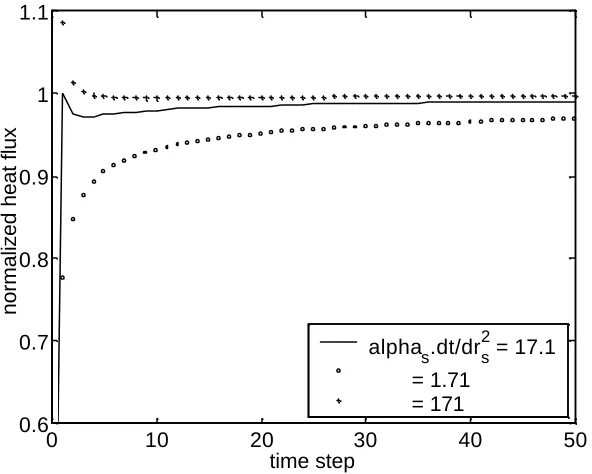
, giving the heat transfer rates shown in Fig. 4. When αs∆t/∆rs 2

=17.1, the finite difference heat flux solution reached the correct value immediately after the start of heating. The magnitude of the heat flux then decayed slightly, passed through a turning point and asymptotically approached the correct value. This case will be referred to as critical discretization. For αs∆t/∆rs

2

>17.1, there was an initial overshoot and for αs∆t/∆rs 2

<17.1, the solution approached the final (correct) value relatively slowly.

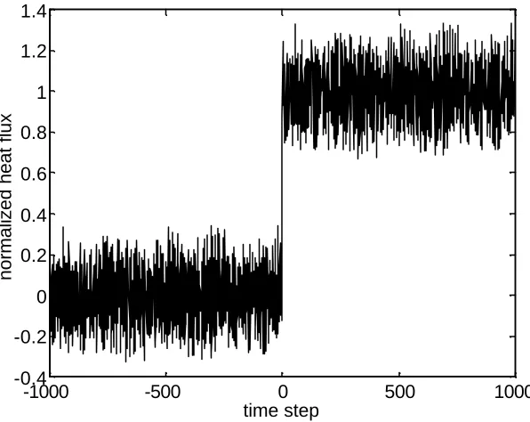
Actual thin film temperature measurements will be contaminated with some degree of electrical noise. To examine the performance of the routine under such conditions, heat flux results were obtained (e.g., Fig. 5) when random fluctuations were superimposed on the temperature history. Results from these calculations are presented in Fig. 6.

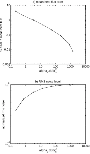
From Fig. 6, it appears that using a value for αs∆t/∆rs 2

=17.1 results in an acceptable error (around 0.5 %) in the mean heat flux level. For values of αs∆t/∆rs

2

>17.1, smaller errors are produced. However, as an accuracy of around 0.5 % is better than the uncertainties in the heat flux which arise from possible deviations in the thermal properties of fused quartz (see Appendix A, or Buttsworth and Jones, 1998), the use of values of αs∆t/∆rs

2

>17.1 is not justified. Furthermore, when the value of αs∆t/∆rs 2

is increased, the noise level associated with the calculation also increases (Fig. 6b). However, it is not possible to greatly reduce (and thereby lower the noise level) without compromising the accuracy of the solution (Fig. 6a). Using a value αs∆t/∆rs

2

=17.1 of appears to be a reasonable compromise between the relatively low frequency accuracy of the solution and the noise level associated with the discretization. In its present form, the routine calculates the required discretization (∆rs) based on the temperature data sampling rate (∆t) using αs∆t/∆rs

2 =17.1.

3.2. Radius of Curvature

approximations made in the derivation of the analytical result which are discussed by Buttsworth and Jones (1997).

3.3. Varying Thermal Properties

To verify the implementation of the variable thermal property form of the one dimensional heat conduction equation (Eq. 4), comparisons were made with an analytical solution. Yang (1952) examined the case of a semi-infinite flat plate subjected to a step change in surface temperature, when the conductivity was a function of temperature, but the specific heat (and the density) was constant. Under these conditions, the diffusion equation can be transformed into the second order nonlinear ordinary differential equation,

0 2 1 2 2 2 = +         + _∗ ∗_{∗ ∗}∗ _∗∗ _∗∗ ∗ ∗ dy d k y dy d d dk k dy

d θ θ

θ θ

(15)

with the boundary conditions θ∗_{(0) =1}

θ∗ _{(∞) =0}

Equation (15) may be written as the system of coupled first order ordinary differential equations,

∗ ∗ ∗ ∗ ∗ ∗ ∗ ∗ ∗ − − = 1 2 1 2

1 1 _θ 2 _θ

θ θ k y d dk k dy d (16a) ∗ ∗ ∗ = ₁ 2 _θ θ dy d (16b)

The system described by Eq. (16) can be solved using MATLAB’s differential equation routines using an iterative process (sometimes described as a shooting technique) which involves the selection of the unknown condition, (dθ∗/dy∗)y∗=0so as to satisfy the boundary condition θ∗(∞) = 0.

Calculations of the nondimensional surface temperature gradient were made using the above scheme with the assumption that the conductivity of the substrate was a linear function of temperature given by,

∗ ∗ _{= +aθ}

h 1 (17)

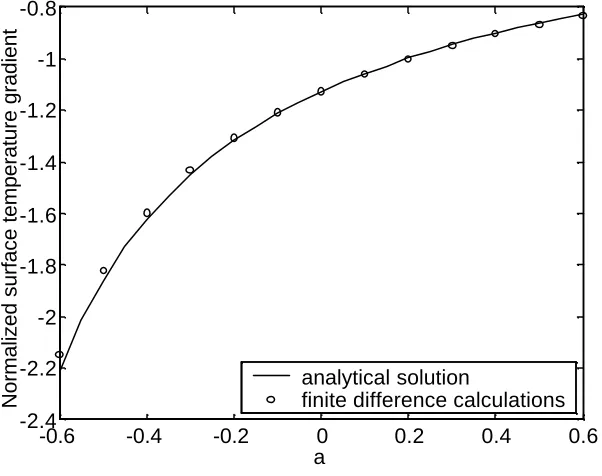
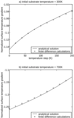
with the value of a varying between −0.6 and +0.6. Results from these calculations are presented as the solid line in Fig. 8. Although the solution of Eq. (15) was obtained though a numerical integration process, the solid line presented in Fig. 8 should be regarded as a faithful representation of the actual solution. This is because the numerical integration and solution process is highly accurate; a test using

k∗=1, yielded the exact solution (dθ∗/dy∗= 2/ π ) to 6 significant figures. Results from the finite difference routine are given by the symbols in Fig. 8. The agreement between the actual solution and the finite difference solution is good. However, the finite difference results are observed to deviate slightly from the actual solution for a<−0.2. At a=−0.6, the finite difference solution is in error by approximately 2.8%. This value of a corresponds to temperature step such that the conductivity at the surface drops to 40% of the value it assumed prior to the temperature step. In practice, a thin film gauge is unlikely to experience such a sever change in conductivity.

0.17%, and this occurred at the temperature step of +200K. These results indicate that finite difference modelling of the variable thermal conductivity of the quartz is likely to be very accurate under realistic test conditions. Under experimental conditions in which the surface temperature of the gauge changes by less than 200K and does so in a relatively slow manner (compared to the step change presently assumed), it is anticipated that the errors introduced by the finite difference calculation for variable thermal conductivity will be less than 0.3%. Such an error is an order of magnitude lower than the uncertainty in the actual value of the thermal conductivity for the quartz gauge (see Appendix A).

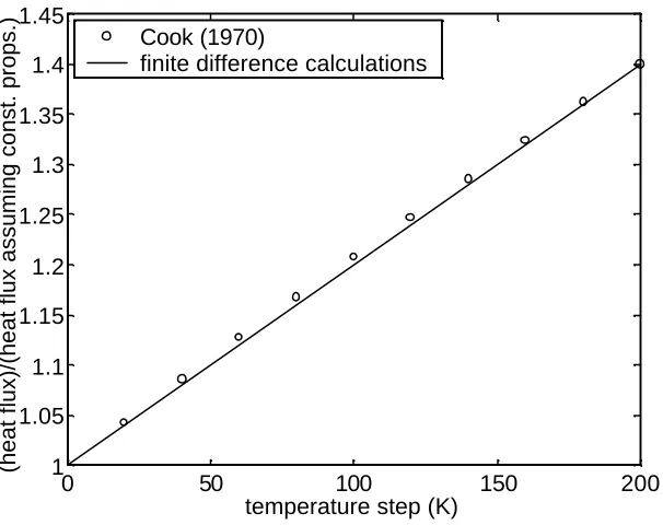
So far, only variations in the substrate conductivity have been considered. To test the performance of the routine when both k, and c vary with temperature, the results presented by Cook (1970) were considered. Cook calculated the heat flux using the Hartunian and Varwig (1962) thermal properties for Pyrex for both a surface temperature step and a parabolic surface temperature history. Linear regressions for the Hartunian and Varwig Pyrex data are,

c = 1.2928 T + 390.64 (18)

k = 7.3854×10-3 T −0.85981 (19)

were T expressed in K gives c in J.kg-1.K-1 and k expressed in W.m-1.K-1.

Calculations were performed using the finite difference routine with values of c and k given by the above expressions for surface temperature steps and an initial (pre-step) temperature of 21°C. (The density of Pyrex was taken as 2220kg.m-3.) Results are compared with those of Cook in Fig. 10. The observed agreement with the calculations of Cook is very good. Small differences do exist, however these are easily accounted by errors associated with determining the magnitude of the previously calculated values (from figure 2 in Cook, 1970).

4. Conclusion

References

Anderson, J. D., 1989, Hypersonic and High Temperature Gas Dynamics, McGraw-Hill.

Buttsworth, D. R., and Jones, T. V., 1997, “Radial Conduction Effects in Transient Heat Transfer Experiments,” Aeronautical J., Vol. 101, No. 1005, 209-212.

Buttsworth, D. R., and Jones, T. V., 1998, “A Fast-Response Total Temperature Probe for Unsteady Compressible Flows,” J. Engineering for Gas Turbines and Power, Vol. 120, No. 4, 694-702.

Cook, W. J., 1970, “Determination of Heat-Transfer Rates from Transient Surface Temperature Measurements,” AIAA J., Vol. 8, No. 7, 1366-1368.

Hartunian, R. A., and Varwig, R. L., 1962, “On Thin-Film Heat-Transfer Measurements in Shock Tubes and Shock Tunnels,” Physics of Fluids, Vol. 5, No. 2, 169-174.

Kemp, N. H., Rose, P. H., and Detra, R. W., 1959, “Laminar Heat Transfer Around Blunt Bodies in Dissociated Air,” J. Aero/Space Sci., Vol. 26, 421-430.

Miller, C. G., 1981, “Comparison of Thin-Film Resistance Gages with Thin-Skin Transient Calorimeter Gages in Conventional Hypersonic Wind Tunnels,” NASA TM-83197.

Schultz, D. L., and Jones, T. V., 1973, “Heat-Transfer Measurements in Short-Duration Hypersonic Facilities,” Agardograph No. 165.

Touloukian, Y. S. (Ed.), 1970, Thermophysical Properties of Matter, The TPRC Data Series, Vol. 2, Thermal conductivity nonmetallic solids, and Vol. 5, Specific heat nonmetallic solids, Ifi/Plenum.

White, F. M., 1991, Viscous Fluid Flow, 2nd. ed., McGraw Hill.

Figures

x

r

R

+ q

gold leads

platinum thin film

Figure 1. Typical arrangement of a platinum thin film heat flux gauge.

r m

m-1 m+1 n-1 n

1 substrate surface

centre of substrate ∆r ∆r_s

0 0.2 0.4 0.6 0.8 1 0

2 4 6 8 10 12 14 16 18

radial location, r/R

dr/dr

s

Figure 3. Distribution of the finite difference node spacing illustrating grid refinement towards the surface.

0 10 20 30 40 50

0.6 0.7 0.8 0.9 1 1.1

time step

normalized heat flux

alpha_s.dt/dr_s2 = 17.1 = 1.71 = 171

Figure 4. Finite difference calculations of heat flux for three values of the discretization parameter (αs∆t/∆rs

2

-1000 -500 0 500 1000 -0.4

-0.2 0 0.2 0.4 0.6 0.8 1 1.2 1.4

time step

normalized heat flux

Figure 5. Finite difference heat flux results when random fluctuations are imposed on the temperature history for αs∆t/∆rs

0.1 1 10 100 1000 10000 0.001

0.01 0.1 1 10

alpha_s.dt/dr_s2

% error in mean heat flux

a) mean heat flux error

0.1 1 10 100 1000 10000

10-1 100

alpha_s.dt/dr_s2

normalized rms noise

b) RMS noise level

Figure 6. Results from the routine with random fluctuations imposed on the surface temperature history. a) Percentage error in the mean heat flux level after the step in heat flux; b) RMS noise levels

(prior to the heat flux) normalised using the corresponding RMS value for the case αs∆t/∆rs 2

0 0.05 0.1 0.15 0.2 0.5

0.6 0.7 0.8 0.9 1

alpha.t/R2

(heat flux)/(flat plate heat flux)

cylinder

sphere

Figure 7. Results from the finite difference routine (solid lines) and the approximate analytical solution (symbols) for curvature effects.

-0.6 -0.4 -0.2 0 0.2 0.4 0.6

-2.4 -2.2 -2 -1.8 -1.6 -1.4 -1.2 -1 -0.8

a

Normalized surface temperature gradient

analytical solution finite difference calculations

0 50 100 150 200 -1.14

-1.12 -1.1 -1.08 -1.06 -1.04 -1.02

temperature step (K)

Normalized surface temperature gradient

a) initial substrate temperature = 300K

analytical solution finite difference calculations

-200 -150 -100 -50 0

-1.3 -1.25 -1.2 -1.15 -1.1

temperature step (K)

Normalized surface temperature gradient

b) initial substrate temperature = 700K

analytical solution finite difference calculations

0 50 100 150 200 1

1.05 1.1 1.15 1.2 1.25 1.3 1.35 1.4 1.45

temperature step (K)

(heat flux)/(heat flux assuming const. props.)

Cook (1970) finite difference calculations

0 200 400 600 800 1000 0.5

1 1.5 2 2.5 3

temperature (K)

conductivity (W/m/K)

a) conductivity

0 200 400 600 800 1000

0.2 0.4 0.6 0.8 1 1.2 1.4

temperature (K)

specific heat (kJ/kg/K)

b) specific heat

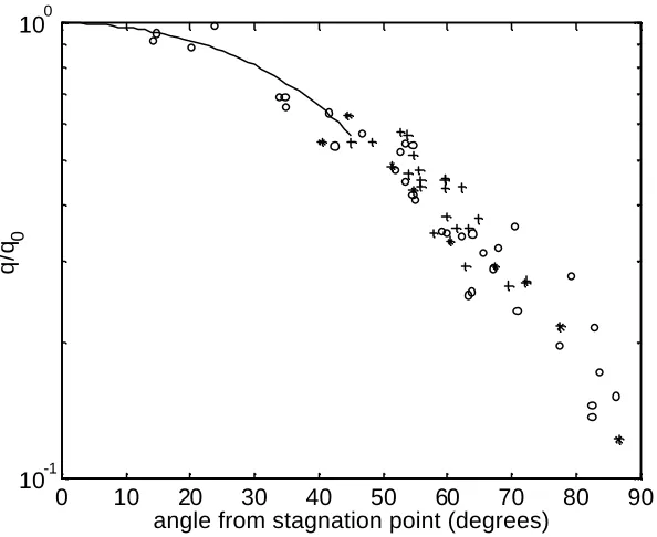
0 10 20 30 40 50 60 70 80 90 10-1

100

angle from stagnation point (degrees)

q/q

0

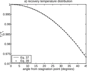
0 5 10 15 20 25 30 35 40 45 0.97

0.975 0.98 0.985 0.99 0.995 1

a) recovery temperature distribution

T r

/T

t

angle from stagnation point (degrees) Eq. 37

Eq. 39

0 5 10 15 20 25 30 35 40 45

0.6 0.65 0.7 0.75 0.8 0.85 0.9 0.95 1

b) convective heat transfer coefficient distribution

h/h

0

angle from stagnation point (degrees) Eq. 40

Eq. 41

Appendices

The finite difference routine was initially developed for hemispherical fused quartz thin film probes (nominal diameter of 3mm) operated in the Oxford University gun tunnel facility (which generates a hypersonic flow lasting approximately 70ms). In the following appendices, some auxiliary functions associated with the finite difference routine are described. Some additional information specific to the Oxford University gun tunnel application is also presented.

A. Thermophysical Properties of Fused Quartz

The thermal properties of materials that are used for thin film heat flux gauge substrates are relatively strong functions of temperature (e.g., Schultz and Jones, 1973). Touloukian (1970) has compiled conductivity and specific heat data for fused quartz from various sources. Recommended values (Touloukian, 1970) for the conductivity of highly pure fused quartz are presented in Fig. 11 along with a 4th order polynomial curve fit to this data. This curve fit is given by the equation,

k = −7.5685×10-12 T4+ 2.2634×10-8 T3−2.1557×10-5 T2+ 9.4079×10-3 T − 5.0808×10-2 (20) where k is in W.m-1.K-1 and T is in K and the valid range is 100 < T < 1000K. Touloukian (1970) states that the uncertainty of the recommended values is thought to be within ± 3 % at temperatures from 200 to 500 K and increase to about ± 8 % at 50 K and 900 K and ± 15 % below 10 K and near 1400 K.

While extensive data for the specific heat of fused quartz as a function of temperature were presented by Touloukian (1970), no recommended values were given. Typical specific heat data from Touloukian (1970) is presented in Fig. 11, along with a 4th order polynomial curve fit for this data. The curve fit is described by the equation,

c = −7.8331×10-10 T4+ 3.3153×10-6 T3−5.3008×10-3 T2+ 4.0143 T − 7.3221×101 (21) where c is in J.kg-1.K-1 and T is in K and again, the valid range is 100 < T < 1000K. Based on an analysis of the deviations in the experimental data (Fig. 11), it is currently estimated that uncertainty of the value of specific heat obtained from the curve fit is within ± 2 % between 200K and 800K. Some researchers have expressed some concern over using bulk substrate values of k and c in the analysis of platinum thin film data (e.g., Miller, 1981). These concerns arise because the substrate properties near the surface are likely to be affected by the diffusion of the platinum thin film into the quartz. However, as such diffusion effects are likely to be limited to the immediate vicinity of the thin film gauge, any deviation in the thermal properties of the substrate will only affect the relatively high frequency content of the heat flux signal. The thermal property values assumed in the current analysis are those given by Eqs. (20) and (21).

B. Stagnation Point Heat Transfer Coefficient

The heat transfer rate at the stagnation point on a sphere in supersonic flow is given by Anderson (1989),

(

)

(

)

dx du

q₀=0.763Pr−0.6 ρ µ 1/2 − (22)

White (1991) gives the similar expression,

(

)

(

)

e e w w e e

e h h

dx du q −     = − 1 . 0 2 / 1 6 . 0

0 0.763Pr _{ρ µ}

µ ρ µ

ρ (23)

Equation (22) has been adopted in the present analysis since it is the slightly simpler expression. The velocity gradient term is estimated using (Anderson, 1989),

e e e p r dx du ρ 2 1 = (24)

since the free stream static pressure will generally be much lower than the pitot pressure (= pe). In the present analysis, r (as opposed to R) refers to the radius of the sphere. Assuming a power law viscosity relationship, n i i T T     = µ µ (25)

and the equation of state given by,

t e e RT p = ρ (26) and that,

(

)

p w

e h c T T

h − = − (27)

where, 1 − = γ γR

c_p (28)

Equation (22) may be written,

(

)

n t n

i

i _{T T}

r p T R T q − −

= −0.6 3/4 ( /2−1/4) 0 1 Pr 907 . 0 γ γ µ (29) That is,

(

)

h

q₀= ₀ − (30)

where, r p T R T

h _tn pit

n i

i 3/4 ( /2 1/4) 6 . 0 0 1 Pr 907 .

0 − −

Using the parameters listed in Table B.1, the value of h₀ r/p_pit was evaluated for helium, hydrogen and nitrogen at a total temperature of 500K (see Table B.1). Since the convective heat transfer coefficient is a relatively weak function of the total temperature (see Eq. 31), the maximum error in the quoted values of h₀ r/p_pit over the temperature range 300 < Tt < 800K (assuming Eq. 31 is

accurate) is approximately ±4%.

Table B.1. Parameters used in evaluating the heat transfer coefficient.

helium hydrogen nitrogen

Pr 0.705 0.706 0.713

µI (N.s.m -2

) 1.870×10-5 8.411×10-6 1.663×10-5

Ti (K) 273 273 273

n 0.666 0.680 0.670

R (J.kg-1.K-1) 2077 4121 297

γ 1.66 1.40 1.40

pit

p r

C. Heat Transfer Coefficient and Recovery Temperature Distribution.

It is reasonable to assume that, at any point around the hemisphere, the gas at the boundary layer edge has a constant entropy since it passed though the normal region of the shock (providing the boundary layers are sufficiently small). Therefore,

( )γ−1/γ

        = pit e t e p p T T (32) and

( )

2 1 /

2 γ γ γ e pit e p p M (33)

Now, since the recovery temperature is defined as,

(

)

r T r M

T γ (34)

it can also be written,

( )

( )

p p T T pit e t

r _{− +}

        = − 1 / 1 γ γ (35)

Assuming that the pressure distribution around the hemisphere is given by the modified Newtonian distribution,

(

)

= p p p

p_{e pit} cos2θ (36)

it is clear that recovery temperature can be expressed as

( )

(

( )

)

T T

t

r _{= 1− cos}2γ−1/γ _{θ+ (37)}

in cases were p∞<< ppit.

The distribution of the heat flux around the surface of the hemisphere can be estimated from the Kemp et al. (1959) data (Fig. 12) as,

2 0

70 . 0

1− θ

= q

q

(38)

Equation (37) can be approximated as,

2 043 . 0

1− θ

= t r T T (39)

when r = 0.85 and γ = 1.4, as shown by the broken lines in Fig. 13. Now because,

t s t s t r T T T T T T h h q q − − = 1 0 0 (40)

2 0

67 . 0

1− θ

= h

h

(41)

D. Lateral Conduction Correction

In general, the heat transfer rate will vary across the surface on which the thin film gauge is mounted. Therefore, lateral temperature gradients are likely to be generated, and lateral conduction may be significant. When significant lateral conduction occurs, it will be necessary to correct the heat transfer results obtained by solving a one dimensional form of the heat conduction equation. In this appendix, two such correction methods are presented. The specific case of a thin film gauge mounted at the stagnation point of a hemispherical substrate in supersonic flow is again considered.

Since the flow (and thus the temperature distributions) will be symmetric about the stagnation point streamline, the equation for heat conduction with constant thermal properties may be written,

t T c T r k r T r k r T k ∂ ∂ = ∂ ∂ + ∂ ∂ + ∂ ∂ _ρ θ2 2 2 2 2 2 2 (42)

The third term on the left hand side of Eq. (4) can be equated to the lateral conduction heat transfer per unit volume, 2 2 2 2 θ ∂ ∂ = T r k

Ql (43)

The normal heat transfer per unit volume will then be given by the remaining terms,

r T r k r T k Q_n ∂ ∂ + ∂ ∂

= 2₂ 2 (44)

The total heat transfer per unit volume being simply,

t T c Q_t ∂ ∂

=ρ (45)

Provided Qn>>Ql, the temperature distribution within the substrate will be largely unaffected by lateral conduction.

To obtain the total lateral heat conduction per unit surface area, Eq. (43) can be integrated from the surface, x = 0 down to a location beyond the heat penetration depth which, for convenience, will be taken as x = R. That is,

∫

R l l Qdx

q

0

(46)

Similarly, the total (convective) heat flux at the surface is simply

∫

∫

t _t dx

T c dx Q q 0 0 ρ (47)

By making the same approximation r≈R (this approximation was used in the derivation of the analytical curvature effects expression, Eq. 3; see also Buttsworth and Jones, 1997) , Eq. (46) becomes,

∫

∫

Therefore, Eqs. (47), and (49) can be substituted into Eq. (48) to obtain

∫

If the convective heat flux at any particular location is reasonably constant with time, the convective heat flux distribution can be modelled by a parabolic distribution such as,

2 0 ) ( θ θ

θ _{A B C}

q

qt _{= + + (51)}

(This is a reasonable approximation in the case of a hemisphere with a sensibly uniform surface temperature distribution, Schultz and Jones, 1973). Therefore,

∫

R

l q d

R C q 0 0 2

4 α τ (52)

Provided the lateral conduction remains a small fraction of the total convective heat flux, the actual

value of q₀ can be approximated in the first instance (q₀o), by the value inferred from the direct (one

dimensional) analysis of the measured temperature history. Thus, a better estimate (q₀i) of the total convective heat flux at the film can be written,

∫

i _{q d}

R C q q 0 0 2 0

0 4 τ

α

(53)

If necessary, Eq. (53) can be used in an iterative manner until convergence is achieved (e.g., for the

next estimate of the actual convective heat flux at the film (qii₀), q₀i would replace q₀o within the integral on the right hand side of Eq. 53). From the Kemp et al. (1959) results described in Appendix C, the value of C is around –0.7.

Method 2

If the convective heat flux changes significantly during a run, then the assumption of a simple parabolic heat flux distribution will probably be inappropriate. However, a correction for lateral conduction can still be obtained by considering the components which contribute to the measured heat flux. In general, both the convective heat transfer coefficient and the flow recovery temperature will vary over the surface of the hemisphere. Thus, it is now assumed that

( )

( ) ( )

h , = ₀ (54)

( )

( ) ( )

r t T t f

T , = ₀ (55)

so that the distribution of surface heat flux can be written

( ) ( ) ( )

(

( )

)

qθ, = θ, _r θ, − _s θ, (56)

It is assumed that the functions fh, fT, and h0 can be determined with sufficient accuracy by other methods (see Appendix B and C).

( )

( ) ( )

T = + (57)

Thus, by substituting Eqs. (54), (55), and (57) into Eq. (56),

( )

( ) ( ) ( )

(

( ) ( )

( ) ( )

)

q , h T 0 T 0 _si 0 s ,

0 θ

θ θ

θ

θ = + − (58a)

The superscript i has been introduced to the stagnation point temperature history to indicate that it should be obtained from the stagnation point heat flux. The stagnation point heat flux q0 is determined from the measured stagnation point temperature history using the finite difference routine which includes variable thermal property effects. However, in the present correction for lateral conduction effects, the spatial distribution of the heat flux is determined using an analysis that includes curvature effects but neglects variable thermal property effects. Thus to preserve compatibility in the present correction analysis, it is assumed that the measured stagnation point temperature history is given by

(

)

T

T_si ₀, , ,

0 = ρ α

(59a)

(

)

(

)

πτ τ

ρ

τ_{erfc s d}

se t q ck t _s

∫

s=− α (59c)

which is, in essence, a rearrangement of Eq. (3).

For simplicity, the functional dependencies will no longer be stated explicitly in each expression. For example, Eq. (58a) will be written,

(

)

h f q f h T h T

f

q 0 0 0

0 −

+

= (58b)

The distribution of surface heat flux, q cannot be determined explicitly from Eq. (58) since the distribution of the surface temperature history, Ts is not known. However, it is possible to determine

q(θ,t) using the following iterative procedure.

1. Make a first estimate of the heat flux distribution using

0

q f f

qi = _{h T} (60)

The first estimate of the surface temperature distribution will therefore be given by,

i s T h i

s f f T

T

0

= (61)

Since it is assumed that lateral temperature gradients are sufficiently small for the substrate temperatures to remain largely unaffected lateral conduction.

2. A better estimate of the surface heat flux distribution can therefore be obtained from Eq. (58) as,

(

)

s i s T T h ii T h T h f q f f

q 0 0 0

0 −

+ =

(

)

s h T h T

hf q f f f h T

f

0 0

0+ 1−

= (62)

The corresponding surface temperature distribution is thus,

(

)

s h T h i s T h ii

s f f T f f f hT

T

0

0 + 1− 0

= (63)

(

)

T_sii _si , , ,

0

0 = 0 ρ α

(64)

from Eq. (59).

3. Again, a better estimate of the surface heat flux can be obtained by substituting the latest estimate of the surface temperature distribution (Eq. 63) into Eq. (58) to obtain,

(

)

(

)

s h T h i s h T h T h iii T h f f f T h f f f q f f q 0 0 0 2 0

0+ 1− + 1−

= (65)

The corresponding surface temperature distribution is thus,

(

)

(

)

s h T h ii s h T h i s T h iii

s f f T f f f h T f f f T

T

0 0

0 1 1

2

0 + −

− +

= (66)

where,

(

)

T_siii _sii, , ,

0

0 = 0 ρ α (67)

from Eq. (59).

4. The last step can be repeated until a sufficiently accurate estimate of q(θ,t) has been obtained. The general result is therefore,

(

)

(

)

(

)

(

)

0 0 0

4 0 0 3 0 0 2 0

0+ − + + + − + +

= iv s iii s T h iii s ii s T h ii s i s T h i s T h

iii _{f f q h T f f hT hT f f hT h T f f h T h T}

q (68)

where

(

)

T_sn _{0 s}n 1, , ,

0

0 ρ α

−

= (69)

and T_si T

(

)

0 = ρ α

(70)

If it is assumed that the functions, _fh and _fT can be written (see Appendix C),

2 1 aθ

f_h = − (71)

2 1 bθ

f_T = − (72)

then at the stagnation point

(

)

(

)

(

)

(

)

(

)

(

)

2

0 0

0 0

0 0 0 0 0

0 0 0 2 2 + + + − + + + + + − =         ∂ ∂ iii s ii s ii s i s i

s a b h T h T a b h T h T

T h q b a q θ (73)

Equation (73) can therefore be combined with Eq. (50) to estimate the lateral conduction since it is presently assumed that ql << qn meaning that the surface heat flux, q ≈ qn. Thus, the lateral conduction is estimated using,

∫

The corrected stagnation point heat flux will therefore be,

If necessary, it is now possible to repeat the whole procedure using the corrected stagnation point surface heat flux in the place of q0 which appears in the above expressions.