City, University of London Institutional Repository
Citation
:
Ribeiro, P., Perra, N. and Baronchelli, A. (2013). Quantifying the effect of
temporal resolution on time-varying networks. Scientific Reports, 3(3006), doi:
10.1038/srep03006
This is the unspecified version of the paper.
This version of the publication may differ from the final published
version.
Permanent repository link:
http://openaccess.city.ac.uk/2832/
Link to published version
:
http://dx.doi.org/10.1038/srep03006
Copyright and reuse:
City Research Online aims to make research
outputs of City, University of London available to a wider audience.
Copyright and Moral Rights remain with the author(s) and/or copyright
holders. URLs from City Research Online may be freely distributed and
linked to.
City Research Online:
http://openaccess.city.ac.uk/
[email protected]
mathematical framework that well describes the behavior observed on real datasets. The analytical description of the bias introduced by time integrating techniques represents a step forward in the correct characterization of dynamical processes on time-varying graphs.
T
ime-varying networks are ubiquitous. Examples are found in the social, cognitive, technological and eco-logical domains as well as in many others1. The temporal nature of such systems has a deep influence ondynamical processes occurring on top of them2–21. Indeed, the spreading of sexual transmitted diseases, the
diffusion of topics over social networks, and the propagation of ideas in scientific environments are affected by duration, sequence, and concurrency of contacts2,4,17–19,22,23. In all these cases the timescale characterizing the
evolution of the network is comparable with the timescale ruling the unfolding of the process, and they cannot be decoupled. However, empirical datasets are often reduced to a series of static networks by introducing a time-integrating window,Dt1,24–27. This is the case, for instance, of face-to-face interaction networks28, for which the
fine-grained temporal resolution of (e.g.) phone call networks is not available, or of infants’ semantic networks29,
whose evolution can be studied only through the analysis of few snapshots30. In other instances, a time window is
introduced to reduce the amount of stored information, or to simplify the application of mathematical frame-works developed for static or annealed systems. This is the case, for example, of online social netframe-works where, although usually the original information has time resolutions down to the second, the available datasets are integrated over different windows of hours, days, months, or even years. Thus, the introduction of an integrating window is either intrinsic to the system under study or dictated by practical reasons.
In this work we address the impact of an arbitraryDton the description of a discrete dynamical process taking place upon a time-varying network. Despite recent results showing that the presence of any level of temporal aggregation may affect the correct characterization of dynamical processes evolving on top of such datasets2–21, an analytical formalization, characterization, and understanding of these effects for a generalDtis still missing.
In particular, we focus on the prototypical random walk process evolving on time-varying networks integrated over a general time windowDt. First, we clarify the relevance of the integrating window issue by studying the behavior of random walk processes on real time-varying networks as a function ofDt. Then, we introduce a mathematical framework that well describes the observed behavior on synthetic activity driven networks17as well as on two different real datasets.
Results
We aim to understand howDtaffects the behavior of dynamical processes taking place on time-varying networks. To this end, we consider the fundamental random walk (RW) process on two different real time-varying networks in which the links have been integrated over different integrating windowsDt(see Fig. 1). Typically, the RW asymptotic occupation probabilityr(see Methods for the formal definition) is computed grouping the nodes according to their the degreek31–33. The quantity r
k is then defined as the average asymptotic occupation
probability of a node in the degree classk31–33. However, in time-varying networks the degree of a node is not univocally defined and, more importantly, is a function ofDt. For example, the degree might be the number of Published
21 October 2013
connections integrated over the time window, or the average number of connections across theT/Dtstatic frames (whereTis the total time span of the data). Thus, the same node could contribute to different degree classes depending on the value ofDt. We, therefore, focus on a different node measure that has been shown to be mostly invariant to
Dt, namely the activity rateaof a node17. The activity rateais defined as the average rate at which each node interacts with others during the observation period [0,T], and can be interpreted as the intrinsic attitude of each node to engage in interactions with other nodes. We aim to calculate the occupation probability as a function ofa.
In our simulations we consider two real time-varying networks, and investigate the RW occupation probability function of activity rateaand the integrating windowDt:ra(Dt). The first dataset is the
co-authorship network of the Physical Review Letters (PRL) journal from 1980 to 200634. The second dataset is the Yahoo! music dataset with,4.6 3105songs rated by,23104Yahoo! users over six months35. We run the RW process over these two time-varying net-works for different values ofDt, and record the occupation probabil-ity over multiple runs (see SI for details). Fig. 2 shows the empirical values ofra(Dt) (solid points) observed in the PRL dataset for four
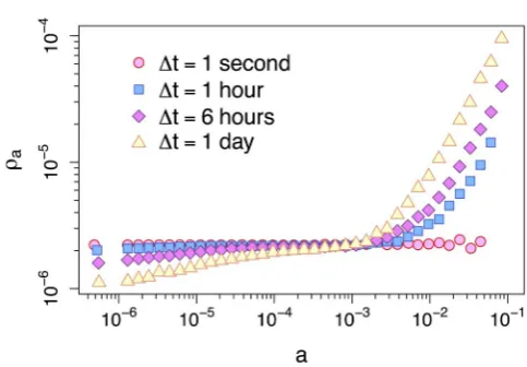
distinct values ofDt5{1, 10, 60, 182} days. Error bars represent the the standard deviation obtained from distinct simulation runs start-ing at timest0g{0, 1, …,Dt21} from the beginning of the dataset. The effect of Dt is dramatic. Over large values ofDt the RW behaves roughly as could be expected. The share of random walkers increases with the node activity, i.e., highly active nodes are collect more walkers at the end of the simulation than nodes with low activity. However, asDtdecreases, more active nodes lose their power to attract walkers and the occupation probability becomes more uniform. A similar scenario is observed over the Yahoo! dataset over four values ofDt, namely one second, one hour, six hours, and one day (points in Fig. 3). In the next section we will see that the reason for this behavior rests solely in the probability that the RW sees no edges when it decides to move, which turns out to be a function of three factors: Dt, the activity of node the walker resides, and the average node activity in the system.
Mathematical formulation.Let us consider a random walker diffus-ing at discrete time steps Dt over a time-varying network charac-terized byNnodes. Starting at nodeV(t) at stept, the walker takes stept11 at time (t11)Dtdiffusing over a networkGt(Dt), where
Gt(Dt) is the result of the union of all the edges generated in the
interval [tDt, (t 1 1) Dt). We focus on the general case of an arbitrary time aggregation windowDt.0.
We consider a simple class of time-varying networks called activity driven networks17. The crucial ingredients of these models are: dF(a), the fraction of nodes with activity ratea, andm, the number of edges that are simultaneously created by a node (see Methods for further details). The activity rate determines the probability per unit time for a node to establish (m, simultaneously) edges to other nodes in the system. The value of parametermis dictated by the specific system under consideration. The casem.1 is appropriate to describe one-to-many interactions, found for example in such systems as Twitter and blog networks36,37. On the other hand,m51 describes two-party (dyadic) communications that are characteristic of phone-call and text-message networks38,39. At each stept50, 1, … an unweighted networkGt(Dt) is generated as follows:
a) Gt(Dt) starts withNdisconnected nodes;
[image:3.595.48.287.49.240.2]b) The the number of times a node with activityaisactiveduring intervalDt,KDt,a, is Poisson distributed
[image:3.595.310.547.53.213.2]Figure 1|Example of time integration on time-varying networks. The random walker is located on the colored node, and can travel on the links depicted as continuous line, whileDtdefines the integration window. Dashed lines represent links that are present in the system, but are out of reach for the walker.
Figure 2|Occupation probabilityraof a RW at the end of the simulation
as a function of node activity. The points are the values ofraof a RW over the Physics Review Letters time-varying co-authorship network from 1980 to 2006 for different integrating windowsDtg{1, 10, 60, 182} days. The error bars are evaluated starting the process at different days from the beginning of the dataset.
Figure 3|Occupation probabilityraof a RW at the end of the simulation
as a function of node activity.Points represent theravalues of a RW over the time-varying graph of Yahoo! song ratings for different integrating windowsDtof one second, one hour, six hours, and one day. The standard deviations are too small to be shown in the plots.
[image:3.595.307.549.520.688.2]and dynamical processes unfolding on their structure .
To describe the RW behavior, we need to evaluate the transition probability that a walker starting at a node with activitya9moves to a node with activityaat the nextDttime step,Qaja9(Dt). Without loss
of generality in what follows we focus on the casem51. Detailed results for them.1 one-to-many interactions are discussed in the Supplementary Information. At stept11 the neighbors ofV(t) can be classified into two types:
1. Passive destinations, are neighbors ofV(t) connected by edges created due to the activity ofV(t) itself. They are randomly selected from the graph and thus their activity is distributed according to dF(a). We defineKDt,A(t)to be the number of such passive destinations, whereA(t) is the activity rate of nodeV(t). 2. Active destinations, are neighbors ofV(t) connected toV(t) by edges created due to their own activity. Thus, their activity is distributed asadF(a)/Æaæ, whereÆaæis the average activity rate in the system. We define defineHDtas the number of such active
destinations.
The worddestinationshighlights the fact that the walker moves from V (t) to one of these KDt,a9 1HDt neighbors of V (t). For
sufficiently largeN,HDtandKDt,a9are both Poisson distributed with averageÆaæDtanda9Dt, respectively. IfV(t) has at least one edge, the walker follows the edge of a passive destination with probability
KDt,a9/(KDt,a91HDt), while it moves towards an active destination
with probability HDt/(KDt,a91 HDt). Unconditioning the latter
expressions with respect to the values ofKDt,a9andHDtwe obtain
Qa aj0ðDtÞ~
X?
k~1
X?
h~0
k
kzhdFð Þa z
h kzh
adFð Þa a
h i
a0Dt
ð Þkðh iaDtÞh
k!h! z
X?
h~1
adFð Þa a
h i
a
h iDt
ð Þh
h! zd a{a
0
ð Þ
!
expð{ða0zh iaÞDtÞ,
ð1Þ
whered(x) is the Dirac delta function. While we refer the reader to the SI for the detailed derivation, each term in eq. (1) has a simple interpretation. The two terms inside the double sum represent, respectively, the probability that the walker moves to a passive des-tination that has activityaand the probability that the walker moves to an active destination that has activitya. The terms multiplying the two terms inside the double summation are related to the probability that KDt,a9 5kandHDt5h. The d(a2a9) term considers the
probability that the node has no edges afterDtand thus the walker must remain atV(t).
Thankfully, eq. (1) can be simplified (see SI) yielding
Qa aj’ðDtÞ~
a’za
a’zh ia dFð Þa 1{fa’,Dt
zdða’{aÞfa’,Dt, ð2Þ
to consider lazy random walks where the walker moves with prob-abilitypg(0, 1] or does not move with probability 12p. For the lazy walker we just need to replaceQaja9(Dt) in eq. (3) withQaja9(Dt)p
1d(a92a)(12p). A simple algebraic manipulation shows thatra
does not change withp. Hence, the steady state of the lazy walker for anypg(0, 1) is the same as the walker that moves with probability
p51.
We also find that closed-form solutions of eq. (3) exist in the limits ofDt?1 andDt=1. In theDt?1 case, links are integrated over a large time window and the time-varying network can be considered static. Recall thatfa,Dt5e(a1Æaæ)Dt. ForDt?1 the value offa,Dt<0, a
gV, and thus the second term of eq. (2) is close to zero. In this scenarioQaja9(Dt)5C(a1Æaæ)dF(a), whereC51/2Æaæyielding the
fixed point solution of eq. (3)
ra< azh ia
2N ah i: ð4Þ
The asymptotic occupation probability of a given node of classais simply proportional to its activity. Since in the regime of largeDtthe degree of a nodev,kv, is proportional to its activity,av, eq. (4) yields rav!kv. Thus, for sufficiently largeDt, we recover the well-known behavior of static networks, where the occupation probability of a node is proportional to its degree31. Furthermore, in the SI we show that eqs. (2), (3), and (4) hold for weighted aggregation procedures where integrated edges have weights proportional to how often they appeared during an intervalDt.
In the regime of very short aggregating windows we have limDtR0
fa,DtR1, agV. Thus, the first term of eq. (2) is zero yielding Qaja9(Dt)5dF(a) and the trivial fixed point solution of eq. (3)
ra<
1
N: ð5Þ
Thus, the walker is equally likely to be found at any node regardless of its activity rate. In fact, whenDtis small the probability a node has more than one edge is close to zero. Consequently, highly active nodes lose and gain walkers at the same rate, giving rise to homo-geneous occupation probabilities in eq. (5). Interestingly, in previous work on general time-varying network processes we show that the result in eq. (5) holds even when aggregated snapshots have arbitrary strong spatio-temporal correlations40.
increasesra/aas predicted by eq. (4), while asDtgets smaller,ra5
1/N, as predicted by eq. (5). The equations describe correctly also the behavior observed for one-to-many simultaneous connections m, characterized by a smoother increase in ra at high activity nodes (seem56 case in Fig. 4, inset). The SI contains more details on the formulation of them.1 case.
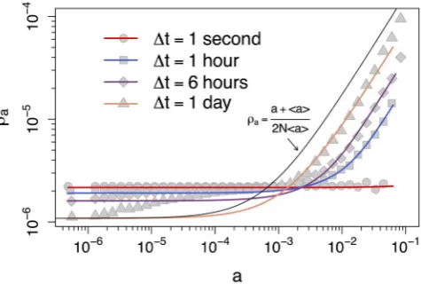
Numerical validation on real-world networks.The analytical frame-work discussed above qualitatively reproduce also the behavior observed in real datasets. In Figs. 5 and 6 the solid lines show the numerical solution obtained by applying eq. (2) into eq. (3) (see SI), for the PRL and Yahoo! datasets, respectively. The gray points in Figs. 5 and 6 reproduce the simulation results already shown in Figs. 2 and 3, respectively. All numerical solutions use the same activity distribution dF(a), extracted from the time-varying graph of
Dt51 day for the PRL dataset andDt51 second for the Yahoo!
dataset (dF(a) extracted from larger values of Dt provide similar results17, see SI for details).
The theoretical results accurately describe real data, with some deviations for nodes in the intermediate activity range atDtof one day. The RW occupation probability is uniform and independent of node activity for smallDtas predicted by eq. (5). As predicted by eq. (4), the RW occupation probabilityraapproaches (a1Æaæ)/(2NÆaæ) (black curve) asDt increases, an effect particularly noticeable for high-activity nodes. It is also worth highlighting that the data matches well the theoretical equations for the casem51, suggesting a connection between the datasets and the fundamental mechanisms described in our model (for the similarity in behavior betweenm51 and projected networks such as the PRL co-authorship networks see SI).
Discussion
Our results clarify the effect of time aggregation procedures on the behavior of the RW, taken as the simplest instance of dynamical process, even when aggregation windows are ‘‘short’’. We have quan-tified this effect in a rigorous mathematical framework that (i) allows us to recover the results concerning static networks in the limit of infinite aggregation windows, (ii) accurately describes the behavior observed in numerical simulations upon synthetic time-varying net-works, and (iii) captures the phenomenology observed on real data-sets. Overall, while for practical or technical reasons researchers are often forced, or simply tempted, to work with time aggregated repre-sentations of time-varying networks, our work suggests that caution should be used when drawing general conclusions about dynamical processes based upon time-aggregated networks. At the same time, moreover, our theoretical results may help to investigate possible distortions introduced by the aggregating windows of data collection methods.
The proposed framework considers inherently discrete processes, such as spreading phenomena in contact networks that are, also at the smallest time resolution possible, discrete. We leave the general-ization to continuous processes for further work.
Methods
Occupation probability.The asymptotic occupation probability is the steady state probability of finding the walker in a node with activitya, which is guaranteed to exist and be unique if the time-varying network that is stationary, ergodic, and connected (see SI), such as in activity driven networks. A time-varying network is T-connected if there is a temporal path between any two nodes40. In our simulations we
[image:5.595.50.289.52.217.2]consider the RW occupation probabilityrato be the probability of finding the walker Figure 4|Occupation probabilityraof a RW over an activity-driven
network with activity distributiondF(a)/a22,ag(1023, 1),N5105, for
different values ofm. Curves in the main plot concern them51 case, where each node can only simultaneously connect to one node. In the inset, the casem56 is considered, where a node simultaneously connect to six other nodes. Solid curves represent the analytical prediction of eq. (3) integrated overDt51, 10, 100 (diamonds, squares and circles) time windows. Note that in both panels asDtgets largerra<a. Averages performed over 103independent simulations.
Figure 5|Occupation probabilityraof a RW at the end of the simulation
[image:5.595.311.549.53.213.2]as a function of node activity.The points are the values ofraof a RW over the Physics Review Letters time-varying co-authorship network from 1980 to 2006 for different integrating windowsDtg{1, 10, 60, 182} days. The solid curves show the respective numerical solutions of eq. (3) and the black curve shows eq. (4).
Figure 6|Occupation probabilityraof a RW at the end of the simulation
as a function of node activity.The points are the values ofraof a RW over the time-varying graph of Yahoo! song ratings for different integrating windowsDtof one second, one hour, six hours, and one day. The solid curves show the respective numerical solutions of eq. (3) and the black curve shows eq. (4).
nodes: authors and papers. An author is connected to all the papers she/he wrote in a integrating windowDt. We study the bipartite projection of the authors. In this representation each author of an article in PRL as a node. Undirected edges connect authors that collaborate in the same article. We focus just on small collaborations filtering out all the articles with more than 10 authors. We consider the period between 1958 and 2006. The datasets contains 80,554 authors and 66,892 articles. The smallest timescale available is one day.
Yahoo! music dataset.In this dataset the bipartite network has two type of nodes: users and songs. We study the bipartite projection over the songs. Each node is a song and two songs are connected if at least one user rated both in a time windowDt. The dataset contains 4.63105songs rated by 199,719 users of Yahoo! users collected in
the course of six months35. User activity is recorded at a time resolution of seconds.
Simulation setup.We obtain the empirical walker occupation probability,ra, as follows. Construct the transition probability matrixPtassociated to the RW on thet -th aggregated networkGt(Dt),t50, …,T/Dt, whereTis the time of the last event in the dataset. The empirical RW occupation probability is obtained by multiplying the matricesP0P1 Pnand then left-multiplying the result by the vector (1/N, …, 1/N), which gives equal probability that for the walker to start at any node. We note in passing that similar results are obtained when the walker starts at a handful of high activity nodes.
1. Holme, P. & Sarama¨ki, J. Temporal networks.Phys. Rep.519, 97 (2012). 2. Morris, M. Telling tails explain the discrepancy in sexual partner reports.Nature
365, 437 (1993).
3. Morris, M. Concurrent partnerships and syphilis persistence: new thoughts on an old puzzle.Sexually transmitted diseases28, 504–507 (2001).
4. Clauset, A. & Eagle, N. Persistence and periodicity in a dynamic proximity network. InDI-MACS Workshop on Computational Methods for Dynamic Interaction Networks1–5 (2007).
5. Vespignani, A. Modeling dynamical processes in complex socio-technical systems.Nature Physics8, 32–30 (2012).
6. Rocha, L. E. C., Liljeros, F. & Holme, P. Simulated epidemics in an empirical spatiotemporal network of 50,185 sexual contacts.PLoS Comput Biol7, e1001109 (2011).
7. Isella, L.et al. What’s in a crowd? analysis of face-to-face behavioral networks.J. Theor. Biol271, 166 (2011).
8. Stehle´, J.et al. Simulation of an seir infectious disease model on the dynamic contact network of conference attendees.BMC Medicine9(2011).
9. Karsai, M.et al. Small but slow world: How network topology and burstiness slow down spreading.Phys. Rev. E83, 025102 (2011).
10. Miritello, G., Moro, E. & Lara, R. Dynamical strength of social ties in information spreading.Phys. Rev. E83, 045102 (2011).
11. Kivela, M.et al. Multiscale analysis of spreading in a large communication network (2011). ArXiv:1112.4312v1.
12. Fujiwara, N., Kurths, J. & Dı´az-Guilera, A. Synchronization in networks of mobile oscillators.Physical Review E83, 025101 (2011).
13. Parshani, R., Dickison, M., Cohen, R., Stanley, H. E. & Havlin, S. Dynamic networks and directed percolation.EPL (Europhysics Letters)90, 38004 (2010). 14. Bajardi, P., Barrat, A., Natale, F., Savini, L. & Colizza, V. Dynamical patterns of
cattle trade movements.PLoS ONE6, e19869 (2011).
15. Baronchelli, A. & Dı´az-Guilera, A. Consensus in networks of mobile communicating agents.Phys. Rev. E85, 016113 (2012).
16. Starnini, M., Baronchelli, A., Barrat, A. & Pastor-Satorras, R. Random walks on temporal networks.Phys. Rev. E85, 056115 (2012).
17. Perra, N., Gonçalves, B., Pastor-Satorras, R. & Vespignani, A. Time scales and dynamical processes in activity driven networks.Sci. Rep.2, 469 (2012). 18. Perra, N.et al. Random walks and search in time varying networks.Phys. Rev. Lett.
109, 238701 (2012).
29. Baronchelli, A., Ferrer-i Cancho, R., Pastor-Satorras, R., Chater, N. & Christiansen, M. H. Networks in cognitive science.Trends in cognitive sciences17, 348–360 (2013).
30. Beckage, N., Smith, L. & Hills, T. Small worlds and semantic network growth in typical and late talkers.PloS one6, e19348 (2011).
31. Noh, J. & Rieger, H. Random walks on complex networks.Phys. Rev. Lett.92, 118701 (2004).
32. Newman, M.Networks. An Introduction157–159 (Oxford Univesity Press 2010). 33. Barrat, A., Barthe´lemy, M. & Vespignani, A.Dynamical Processes on Complex
Networks,160–163 (Cambridge Univesity Press, 2008).
34. American Physical Society. Data sets for research (accessed 2010). URL https:// publish.aps.org/datasets.
35. Yahoo! Webscope dataset (accessed 2012). URL http://labs.yahoo.com/ Academic_Relations.
36. Java, A., Song, X., Finin, T. & Tseng, B. Why we twitter understanding microblogging usage and communities. InIn proceedings of the 9th WebKDD and 1st SNA-KDD workshop on web mining and social network analysis(2007). 37. Kumar, R., Novak, J., Raghavan, P. & Tomkins, A. On the bursty evolution of
blogspace. InIn proceedings of the 12th international conference of world wide web
(2003).
38. Onnela, J.-P.et al. Structure and tie strengths in mobile communication networks.
Proc. Natl. Acad. Sci. U.S.A.104, 7332 (2007).
39. Wu, Y., Zhou, C. J. X., Kurths, J. & Schellnhuber, H. Evidence for a bimodal distribution in human communication.Proc. Natl. Acad. Sci. U.S.A.107, 18808–18808 (2010).
40. Figueiredo, D., Nain, P., Ribeiro, B., de Souza, E. & Towsley, D. Characterizing continuous time random walks on time varying graphs.ACM SIGMETRICS
203–207 (2012).
41. Feller, W.An introduction to probability theory and its applications.Vol. II, (2nd ed.), 334–335 (John Wiley & Sons Inc., New York, 1971).
Acknowledgments
This work was performed while B.R. was a postdoctoral researcher at the University of Massachusetts Amherst visiting the MoBs Lab at Northeastern University. We thank Yahoo! and APS for providing the data used in this work. B.R. was partially supported by the NSF grant CNS-1065133. B.R. and N.P. were partially supported by the ARL Cooperative Agreement W911NF-09-2-0053. The views and conclusions contained in this document are those of the authors and should not be interpreted as representing official policies, either expressed or implied of the NSF, ARL, or the U.S. Government. The U.S. Government is authorized to reproduce and distribute reprints for Government purposes notwithstanding any copyright notation hereon.
Author contributions
B.R., N.P. & A.B. designed research, B.R. & N.P. performed simulations, B.R., N.P. & A.B. analyzed the data, B.R. derived the analytical results. All authors wrote, reviewed and approved the manuscript.
Additional information
Supplementary informationaccompanies this paper at http://www.nature.com/ scientificreports
Competing financial interests:The authors declare no competing financial interests.
How to cite this article:Ribeiro, B., Perra, N. & Baronchelli, A. Quantifying the effect of temporal resolution on time-varying networks.Sci. Rep.3, 3006; DOI:10.1038/srep03006 (2013).