City, University of London Institutional Repository
Citation
:
Sriratanavaree, S., Rahman, B. M., Leung, D. M. H., Kejalakshmy, N. & Grattan,
K. T. V. (2014). Full-Vectorial Finite-Element Analysis of Acoustic Modes in Silica
Waveguides. IEEE Journal of Quantum Electronics, 50(12), pp. 1006-1013. doi:
10.1109/JQE.2014.2364199
This is the accepted version of the paper.
This version of the publication may differ from the final published
version.
Permanent repository link:
http://openaccess.city.ac.uk/12794/
Link to published version
:
http://dx.doi.org/10.1109/JQE.2014.2364199
Copyright and reuse:
City Research Online aims to make research
outputs of City, University of London available to a wider audience.
Copyright and Moral Rights remain with the author(s) and/or copyright
holders. URLs from City Research Online may be freely distributed and
linked to.
City Research Online:
http://openaccess.city.ac.uk/
[email protected]
Full-Vectorial Finite-Element Analysis of
Acoustic Modes in Silica Waveguides
Suchara Sriratanavaree, B. M. Azizur Rahman, Senior Member, IEEE,
David M. H. Leung, Namassivayane Kejalakshmy, and Kenneth T. V. Grattan
Abstract— A finite-element code has been developed to study
the vector acoustic modes in high index contrast silica optical waveguides. Detailed spatial variations of the transverse and longitudinal displacement vectors are shown for the bending, radial, and torsional modes. The variation of the frequency shift due to the stimulated Brillouin scattering and the overlaps seen between the acoustic and optical waveguides also are presented, together with the modal hybridness and modal dispersion.
Index Terms— Acoustic waves, finite element analysis, optical waveguides, stimulated Brillouin scattering.
I. INTRODUCTION
A
COUSTIC waves propagate in a medium due to the periodic displacement of the molecules of which it is composed, being characterized by parameters such as the material density, elasticity, Young modulus, and Poisson’s ratio [1]–[3]. The particle displacement of such a mode in a waveguide can occur in the longitudinal direction or alter-natively in the transverse plane. When the core material in the waveguide is surrounded by a cladding, the propagation of the waves can be classified as being of torsional, bending, radial, flexural or longitudinal type [4], [5]. These modes can be supported, provided at least one of the velocities (the shear or longitudinal velocity) in the cladding exceeds that in the core.It is well known that the acoustic properties of optical waveguides can be coupled to the propagation of light, creating the phenomenon of Brillouin scattering, which in the presence of gain can become Stimulated Brillouin scat-tering (SBS) and allow Guided Acoustic Wave Brillouin scattering (GAWBS) [6]–[8]. The interaction of light with a longitudinal acoustic wave can give rise to either SBS or conventional Brillouin scattering processes. Meanwhile, the transverse acoustic wave interaction may result in GAWBS, which is a relatively weak effect. Analysis of such interactions is not trivial due to the increased complexity of modern optical waveguide structures, exemplified by photonic crystal fibers [8] and sub-wavelength waveguides, such as nanowires. In a way similar to that seen for the hybrid modes in
The authors are with the Department of Electrical Engineering, City Univer-sity London, London EC1V 0HB, U.K. (e-mail: [email protected]; [email protected]; [email protected]; [email protected]; [email protected]).
high-index contrast optical waveguides, the acoustic modes in such optical waveguides are also complex. In these cases, a rigorous full-vectorial analysis [9]–[12] is required for the accurate characterization of the acoustic wave propagation and such a computer code has been developed. In this paper, the development of this code based on the versatile finite element method is reported and numerically simulated results of acoustic wave guiding in a high-index contrast planar silica (SiO2)waveguide are presented and analyzed. The
full-vectorial nature of the acoustic mode in a high-index contrast optical waveguides has been illustrated.
II. THEORY
The propagation of an acoustic wave along the propa-gation direction, z, is associated with a periodic molecular displacement. For a time harmonic wave, the displacement vectors, Ui, can be written in the following form [3]:
Ui=u(ux,uy,j uz)exp{j(ωat−kaz)} (1)
where ux, uy and uz are the particle displacement vectors
along the x , y and z directions, ωa is the angular frequency
representing the time dependence and ka is the propagation
constant identifying the axial dependence. For a loss-less system, uz (the longitudinal displacement vector) is 90 degrees
out of phase with both ux and uy (transverse displacement
vectors). In such a case, by defining uz as an imaginary
component, as shown in Eq. (1), the system equation can be simplified to a real eigenvalue equation. A similar approach has also been exploited for the modal analysis of loss-less optical waveguides [13]. The deformation in an acoustically vibrating body can be described by the strain field, S, where:
S= ∇u (2)
The elastic restoring forces can be defined in terms of the stress field, T. The inertial and elastic restoring forces in a freely vibrating medium are related through the translational equation of motion where:
∇.T=ρ∂
2u
∂t2 (3)
Hooke’s Law states that the strain and stress are linearly proportional to each other and are given by:
Ti j =ci j klSkl; i,j,k,l=x,y,z (4)
The microscopic spring constants, ci j kl, can be termed the
elastic stiffness constants. The compliance and stiffness tensors can be denoted in the matrix form by:
in which ci j kl is a fourth order tensor which obeys the
sym-metry condition and hence can be represented by using two suffix notations. Furthermore, the elastic stiffness constants are related to the shear and longitudinal velocities.
Classically, in the finite element method [14] applied for a solid structure, the displacement field, u, can be written with the help of the interpolation shape function, [N], and of the vector of the nodal values of the displacement field U where:
u = [N]U (6)
u = ⎧ ⎨ ⎩ ux uy uz ⎫ ⎬ ⎭ = ⎡
⎣N10 N10 00 0 0 N1
N2 0 0 0 N2 0 0 0 N2
N3 0 0 0 N3 0 0 0 N3
⎤ ⎦ ⎡ ⎢ ⎢ ⎢ ⎢ ⎢ ⎢ ⎢ ⎢ ⎢ ⎢ ⎢ ⎢ ⎣
u1x
u1y u1z u2x
u2y
u2z u3x
u3y
u3z
⎤ ⎥ ⎥ ⎥ ⎥ ⎥ ⎥ ⎥ ⎥ ⎥ ⎥ ⎥ ⎥ ⎦ (7)
The general system of equations associated with this problem can be written as:
([A] −ω2a[B])U=F (8) where [ A] is the stiffness matrix which is related to strain energy and [B] is the mass matrix related to the kinetic energy. These matrices are generated for a given propagation constant, ka. The column vectors, F, contain the nodal values
of the applied forces, which in this case are taken to be equal to zero. Solving this generalized eigenvalue equation for this system yields an eigenvalue which is ωa2, where ωa is the
angular frequency and the eigenvector U is the displacement vector. From the given input ka and output ωa, the phase
velocity of the acoustic wave, va, can be calculated from the
following relationship:
va=ωa/ka. (9)
The associated boundary condition of the fully-vectorial displacement vector is similar to that of an electric wall on the electromagnetic field.
III. RESULTS ANDDISCUSSIONS
Initially, the computer code developed has been bench-marked to study torsional and bending modes of a high-index contrast steel waveguide [15] and also a low-index contrast silica fiber [16]. The agreements seen were very good, but these are not shown here.
A. Silica (SiO2)Waveguide Analysis
Silica (SiO2) is the most widely used material for optical
waveguides because of its extremely low loss value and in this study a simple rectangular SiO2 waveguide is
[image:3.612.319.555.54.227.2]consid-ered, where its longitudinal and shear velocities are taken as 5736 m/s and 3625 m/s, respectively [5]. A low acoustic
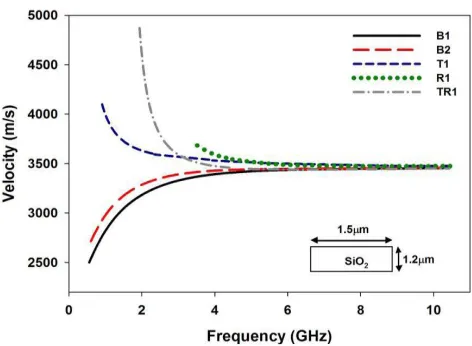
Fig. 1. Variations of phase velocities with the frequency for different acoustic modes.
index material (with larger acoustic velocities) is needed as the surrounding cladding material to allow the guidance of both the longitudinal and shear modes. In this case, the well-studied example of xenon gas is considered, as this is known to support both longitudinal and transverse modes. The longitudinal and shear wave velocities in xenon are taken as 22303 m/s and 15472 m/s, respectively [17]. Any optical material with similar higher longitudinal and shear velocities is expected to give similar acoustic modes. The horizontal (width – W) and vertical (height – H) dimensions of the SiO2 waveguide are
initially taken as 1.5μm and 1.2μm, respectively.
The most important modal parameter, the modal dispersion properties of an acoustic waveguide shows the relationship between the frequency or the angular frequency, propagation constant and phase velocities. Variations of the modal phase velocities with the frequency for the first 5 modes are shown in Fig. 1. In this case, 12000 first order triangles were used to represent the waveguide structure. These are identified as Bending 1 (B1), Bending 2 (B2), Torsional (T1), Radial (R1) and Torsional-Radial (TR1) modes. Their detailed mode profiles are shown later in the paper. It can be observed that for the two bending modes, as the modal frequency is increased, their phase velocities increase and asymptotically approach the Rayleigh wave velocity. Later it will be shown that as the wavenumber or the frequency is increased, the modal displacements move closer to the interfaces. These surface waves propagating along the interface of a solid are also known as Rayleigh waves. By contrast, for the torsional, radial and torsional-radial modes, as the modal frequency is increased, their phase velocities decrease and asymptotically reach the Rayleigh wave velocity. The waveguide cross-section is shown in Fig. 1 as an inset.
It can be observed that the phase velocity of the B1 mode is lower than that of the B2 mode for a given propagation constant, ka. In this case, the width (W) of the waveguide
was taken as being larger than its height (H) and the B1 mode with the Uy displacement vector is seen as the
dominant component: this can also be termed the Uy mode, where as for the B2 mode with its Uxdisplacement vector as
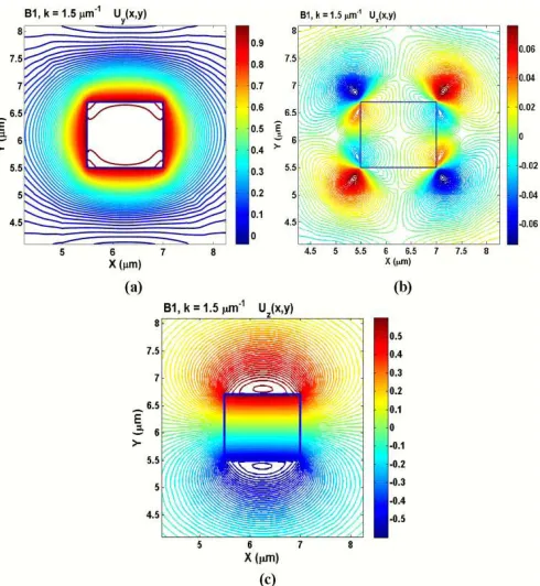
Fig. 2. The displacement vector plots (a) Ux(b) Uy, and (c) Uzcomponents
of B1 mode (Uy) at ka=1.5μm−1.
In this case, as their width and height were not equal, the Ux and Uy modes were not degenerate and it was possible to isolate them when the full structure was considered in the simulation. However, in the case when the height and the width of a waveguide are identical, these two B1 and B2 modes will be degenerate and in that case, the symmetry condition can be imposed along the vertical and horizontal axes (through the center of the waveguide) to isolate these degenerate modes. For this waveguide, with W =1.5μm and H=1.2μm, and the propagation constant, ka = 2.0 μm−1, the frequency of
the B1 or Uy mode was 0.8716 GHz and that of the B2 or Ux mode was 0.9362 GHz. However, if the waveguide height and width are identical, the Ux and Uy modes will be degen-erate, as for W = H = 1.2 μm and ka = 2.0 μm−1, both
the frequencies have been calculated as 0.880 GHz and for the same value of ka, this parameter will be 0.929 GHz when
W = H =1.5 μm. This indicates that the frequency of the fundamental Uymode is more related to the waveguide height and that of the fundamental Ux mode is clearly related to its width.
B. Modal Field Profile
1) Bending Mode: The full-vectorial mode profile of the
B1 mode is shown in Fig. 2, for the case when ka=1.5μm−1.
For this mode the dominant displacement vector was Uyand
its spatial variation in the x –y plane is shown in Fig. 2(a). It can be observed that the Uy profile is strongly confined
inside the waveguide with almost a constant value and this reduces monotonically in the cladding. Its detailed variation along the transverse coordinates will be shown later. The variation of the non-dominant Uxprofile across the waveguide
[image:4.612.53.298.57.323.2]cross-section is shown in Fig. 2(b). It can be observed that its
Fig. 3. Variations of Ux and Uy along the x-axis for B1 and B2 modes,
respectively at ka=1.5μm−1.
magnitude is relatively small, at only 6% of the dominant Uy displacement vector, and clearly shows a higher order
spatial variation at the four corners of the waveguide. The spatial variation of the Uz vector for this mode, B1, is shown
in Fig. 2(c), which clearly shows both positive and negative peaks along the upper and lower horizontal side walls. The waveguide outline is also illustrated in these figures. The magnitude of the Uz displacement vector is considerable
higher, at about 60% of the dominant Uy vector. It is well
known that in optical waveguides with a strong refractive index contrast, all the 6 components of the electric and magnetic fields exist [18] and a similar feature for an acoustic waveguide with a strong material contrast is also demonstrated here. It should be noted that for the quasi-TE or Hy11 mode of an optical waveguide [19], its Hy field is the dominant
component and is primarily confined inside the waveguide core. For the smaller non-dominant Hx field, this is mainly
located around the four corners of the waveguide with higher order spatial variations. The parameter Hz has a relatively
higher magnitude but with its peaks along the upper and lower dielectric interfaces, this strongly correlates with the eigenvector shown in Fig. 2 for the Uy mode.
The B2 mode has the Ux component as its dominant
displacement vector (this is not shown here) with its profile similar to that of the Uyprofile for the Uymode (or B1 mode),
(which is shown in Fig. 2(a)). Similarly, the non-dominant Uy
component of this B2 mode (with Ux dominant) has higher
order spatial variations at the waveguide corners with only 6% of the magnitude. Its Uz profile is also similar to the
Uz profile of the B1 mode (with Uy dominant), which is
shown in Fig. 2(c), but for this mode rotated 90 degrees, with its positive and negative peaks along the left and right vertical interfaces (but these are not shown here). Its maximum magnitude is about 60% of that the dominant Uxcomponent.
For this Ux mode (or B2 mode) with the dominant Uxvector,
this strongly correlates with the eigenvector profile of the fundamental Hx11 (quasi-TM) mode in an optical waveguide with a strong index contrast, such as a silicon nanowire.
Variations of the Uy displacement vector for the Uy mode
[image:4.612.311.561.58.229.2]Fig. 4. Variation of Uy of the Bending, B1(Uy) mode along y-axis for ka=1.5μm−1and ka=2.0μm−1.
along the x -axis are shown in Fig. 3, when ka =1.5 μm−1.
The Uy profile inside the core, shown by a dashed line,
is nearly flat inside the core but with small ripples and a smaller peak at the center (shown as an inset), where its value reduces rapidly outside the core. On the other hand, the Uxprofile, shown by a solid line, is also nearly flat inside the
core but with a small dip at the center (shown as an inset) and outside the core its value reduces more rapidly and is associated with the small negative values. For this waveguide, as the material contrast was very high, the modal eigenvectors shows strong confinement inside the core. For a smaller index contrast, such as with a Ge doped SiO2waveguide with SiO2
cladding, it has been observed (but is not shown here) that the variations of Ux and Uy along the transverse directions are
slower and can be close to a Gaussian profile in shape. The variation of the Uydisplacement vector for the Uymode
(B1) along the y-axis is associated with a small negative dip outside the core (similar to the Uxprofile of the Uxmode (B2)
along the x -axis as shown in Fig. 3), but this is not shown here. Similarly, the variation of the Uxdisplacement vector for
the Ux mode along the y-axis is monotonic without changing its sign, in a way similar to the Uy profile along the x -axis
(as shown in Fig. 3) for the Uy mode. Thus the dominant Uy and Ux profiles of the Uy and Ux modes reverse the
nature of their variations along the x and y directions. When the waveguide width and height are equal, the Uxand Uy modes are degenerate. As a result, the modes can easily exchange power between them. For two degenerate modes with the magnitudes of Ux and Uy (and these being equal),
their resultant displacement vectors are oriented at 45 degrees to the two perpendicular axes. As the axial propagation constant, ka, increases, these mode shapes transform slowly
and become more confined and the magnitudes of the non-dominant components also increase.
The Uy profiles along the y-axis for the Uy mode (B1)
are shown in Fig. 4, for two different ka values. It can be
observed that when the propagation constant is increased, the field outside the core reduces more rapidly – here the negative peak gets slightly larger, but it moves closer to the boundary. A larger dip at the center of the waveguide exists for the
[image:5.612.317.558.56.228.2]Fig. 5. Variation of the Uyof B1 mode along y-axis at ka=4.0μm−1and ka=10.0μm−1.
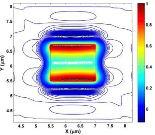
Fig. 6. Uyprofile of the Bending mode (B1) at ka=10.0μm−1.
larger ka value, given by ka = 2 μm−1. Similarly, its (Uy)
variation along the x -axis also becomes faster outside the core when the propagation constant, ka, is increased, (but this is not
shown here). As the value of kais increased, the non-dominant
displacement vector, Ux for the B1 mode also becomes more
confined near the 4 corners and its magnitude is increased, as is seen for example from 6% at ka=1.5μm−1to 10% when
ka=4.0μm−1.
Variations of the Uyprofile along the y-axis, for two even
higher values of the propagation constant, ka = 4.0 and
10.0 μm−1, are also shown in Fig. 5 for the B1 mode. It can be observed that as the ka value is increased, the dip at
the center increases further and now the eigenvector is more confined along the upper and lower horizontal interfaces of the waveguide. The negative dip outside the core also becomes slightly larger, sharper and closer to the waveguide interfaces. The transverse variation of the displacement vector, Uy,
of the Uy mode (B1) across the waveguide cross-section is shown in Fig. 6, when ka = 10.0 μm−1. It can be
observed that the profile of Uy for the same B1 mode at ka = 10.0 μm−1, as shown here, is quite difference from
the Uy profile at ka = 1.5 μm−1, as shown in Fig. 2(a).
[image:5.612.361.517.272.408.2]Fig. 7. Variation of Uzalong y-axis of the B1 mode(Uy) at ka=1.5μm−1
and ka=4.0μm−1.
propagation constant, the magnitude of the non-dominant Uxdisplacement vector of this B1 mode increases significantly
to about 40%, but their displacements are mainly confined at the four corners of the waveguide, (which is not shown here). The variations of the axial displacement vector, Uz, for the
B1 (Uy) mode along the y-axis for ka = 1.5 and 4.0 μm−1
are shown in Fig. 7. It can be observed that as the propagation constant is increased, the displacement vector Uz becomes
more narrowly confined along the upper and lower horizontal interfaces and its magnitude also slightly increases.
The detailed spatial variations of all the three displacement vector components for this B1 (Uy) mode are shown in Figs. 2 to 7. For the B1 (or Uymode), the displacement vector has the dominant Uy component and the resultant structural
deformation will be in the vertical direction, particularly for lower propagation constants (or lower frequencies). However, for higher frequencies, as the magnitude of the Ux
displace-ment also increases to nearly 40% of the Uy displacement,
the profile of their combined transverse displacement vector (Ut = xUx +yUy) will modify considerably, particularly
near the four corners. The signs of the displacement vectors will change after every half-wavelength and repeat after every wavelength and this will produce a periodic structural bending along the vertical axis. Similarly, for the B2 mode, the periodic displacement along the x -axis will cause this mode to periodically bend the waveguide along the x -axis.
It should be noted that for the B1 mode, although the dominant displacement is in the y-direction, it also has a significant Uz displacement. The variation of Uz along the
transverse plane is more complicated with its positive and negative values at the upper and lower horizontal interfaces. The total displacement will vary periodically along the axial direction. As ka increases, both the dominant Uy and the
next significant component, Uz, are confined mainly along the
upper and lower horizontal interfaces and like a surface mode confined along the material interfaces, its velocity approaches that of the Rayleigh wave.
2) Torsional Mode: The modal properties of other modes
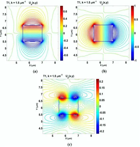
are of interest and are presented briefly. The torsional mode, labeled T1 in Fig. 1, has nearly equal Ux and Uy
displace-Fig. 8. Displacement vector (a) Ux(b) Uy, and (c) Uzprofiles of the T1 mode
at ka=1.5μm−1.
ment vectors. The Ux, Uy and Uz profiles for this mode at ka = 1.5 μm−1 are shown in Fig. 8. It can be observed
that the more dominant displacement vector, Uy shows its
maximum values along the left and right vertical interfaces, as shown in Fig. 8(b). On the other hand the horizontal displacement vector, Uxshows its maximum values along the
upper and lower horizontal interfaces, as shown in Fig. 8(a). As the height and width of the waveguide were not equal, the torsional modes were not degenerate and the magnitudes of the Uxand Uyvalues were also slightly different. The Uz profile
of this torsional mode (T1) is shown in Fig.8(c) – this exists mainly at the four corners with higher order spatial variations. For this ka value, its magnitude was 20% of the dominant
Uy components, and this shows that the relative magnitude
of the longitudinal displacement vector, Uz, is lower than that
of the B1 and B2 modes. This mode shows antisymmetric Ux
and Uy displacement vectors and the Uz displacement vector
with very small magnitude will have a smaller interaction with the fundamental optical mode.
The combined displacement vector, Ut in the transverse
plane for this torsional mode, T1, is shown in Fig. 9, when
ka =1.5 μm−1. This clearly shows a twist in the transverse
plane due to the combination of the x and y displacement vectors, which has been shown in Fig. 8(a) and (b), respec-tively. Every half-wavelength, the sign of the displacement vectors (and direction of twist) will change. This will give the periodic clockwise and anticlockwise twists in the transverse plane along the waveguide.
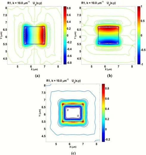
3) Radial Mode: By contrast, the radial mode R01 labeled R1, shows a considerable magnitude for all the three displace-ment vectors. The Ux, Uy and Uz profiles for this mode at ka = 10.0 μm−1 are shown in Fig. 10. It can be observed
[image:6.612.316.561.58.316.2]Fig. 9. The vector displacement, Ut plot of Torsional mode (T1) at ka=1.5μm−1.
Fig. 10. The displacement vector plots of (a) Ux (b) Uy and
(c) Uzcomponents of the R1 mode at ka=10.0μm−1.
in Fig. 10(b), is mainly confined to the upper and lower hori-zontal interfaces. On the other hand, the Uxdisplacement
vec-tor, shown in Fig. 1 (a), is mainly confined along the left and right vertical interfaces with its maximum magnitude being about 80% of the maximum Uy displacement. However its
Uz profile, given in Fig. 10(c), clearly shows its confinement
along all the four interfaces with the sharp peaks at the four corners. It changes its sign at the interfaces and sustains a smaller but relatively constant magnitude inside the core. Its maximum magnitude is 80% (of that of the dominant Uy
displacement vector) at the four corners, about 50% along the four interfaces and about 25% inside the core. Due to the symmetric nature of the Uz profile, this mode would be
expected to have a considerable overlap with the fundamental optical mode.
4) Torsional-Radial Mode: Figure 11 (a) shows the resultant
Ut vector profile in the transverse plane for the R1 mode
Fig. 11. Vector plot Ut of (a) Radial mode (R1) (b) Torsional-Radial
more (TR1) at ka=10.0μm−1.
when ka = 10 μm−1. In this case, the dominant Uy had
positive and negative peaks at the upper and lower interfaces, as shown in Fig. 10 (b) and Uxhad negative and positive peaks
along the left and right interfaces as shown in Fig. 10 (a). The resultant Utvector shows a displacement which moves radially
outward but is periodically reversing its direction so expanding and contracting its dimension along the propagation direction. However, its changing cross-section remains rectangular in shape. R1 will perturb the refractive index profile radially without changing the polarization of the guided wave. The combination of the transverse and longitudinal displacements can give rise to nonlinear optical effects such as SBS and polarized GAWBS [7], [20].
The Ux and Uy profiles of the TR21 mode, labeled as
the TR1 mode, were similar to that of the R1 mode, but
π radian out of phase in the time axis (and these are not shown here). However, their out of phase combination yields the Ut profile, which is shown in Fig.11(b). This shows the
maximum displacement in the four quadrants of the core. The vector displacement shown in this figure will cause the guide to expand along the vertical axis and ‘squeeze’ along the horizontal axis. This produces a deformation of the waveguide which also reverse its shape periodically and hence induces additional optical birefringence.
C. Acoustic-Optical Interactions
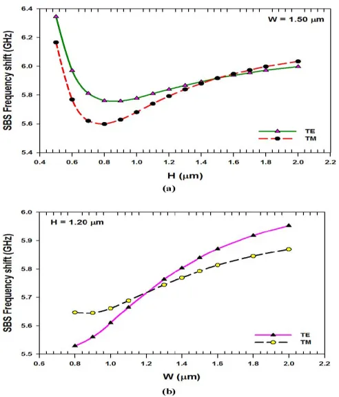
1) SBS Shift Frequency: In this section the interaction
between the acoustic and the optical mode has been studied by using ka=2β to calculate the SBS frequency shift in the
acoustic waveguide and afterwards the overlap integrals of the acousto-optic interaction are shown [21]–[23].
[image:7.612.317.561.59.200.2] [image:7.612.52.297.239.500.2]Fig. 12. Variation of the SBS frequency shift (GHz) with (a) Height (μm) and (b) Width (μm) for quasi-TE and quasi-TM modes.
It can also be noticed that as the width is increased, the SBS frequency is increased of both quasi-TE and TM modes, as it approaches the maximum width the quasi-TE mode has higher SBS frequencies than that quasi-TM mode, of 5.98 GHz and 5.85 GHz, respectively.
2) Modal Overlap: As discussed previously, the SBS
frequency indicates the resulting frequency shift due to the optical-acoustic interaction: however, its strength depends on the overlap between these modes. The overlap interaction of the transverse Radial (R1 or Uy12)mode with its Uz
displace-ment vector is shown here. The variation of overlap integral values of the acousto-optic interaction is shown in Fig. 13(a). This represents the overlap interaction of the Uzdisplacement
vector with the dominant optical field. For the quasi-TE mode, the overlap integral determination was carried out with the dominant Hy field, but for the quasi-TM mode, it was done
with the Hx field. In here, the overlap calculation of the
Uz displacement vector profile of the radial mode will
intro-duce both GAWBS and SBS into the core of the waveguide and create the interaction between acoustic and optical modes. The graph shows that the maximum overlap is achieved when the heights are 1.0 μm and 1.15μm for the quasi-TE and quasi-TM modes, respectively, and further increases of height will reduce the overlap integral. Therefore, the mismatch between the acoustic and the optical mode is higher when the height is increased. In this section the effect of the width of the SiO2waveguide is studied on the SBS frequency
[image:8.612.319.556.54.340.2]shift and the overlap between the acoustic and optical waves. To achieve that, first the optical modes are studied. To obtain the SBS frequency shift, it is essential to calculate
Fig. 13. The overlap variations with the (a) Height (μm) and (b) Width (μm) of the guide for the quasi-TE and quasi-TM modes.
the propagation constant, which is related to the effective index of a mode. Figure 13 (b) shows the overlap integral between the acoustic radial mode (R1) of its Uz displacement vector
with the fundamental quasi-TE and quasi-TM optical modes with the waveguide width. It can be observed that as the width of the guide is increased the overlap increases rapidly and reaches its maximum value, then reduces as width is increased further. When the width is at its maximum, the overlap ratio between acoustic and optical modes is at its minimum. In contrast, a higher overlap ratio is shown to be 0.438 and 0.40 at 1.1 μm and 1.15 μm, respectively, for the quasi-TE and quasi-TM modes. It can be observed that the mismatch between acoustic and optical waves is quite high when width is increased.
IV. CONCLUSION
Detailed displacement vectors for several fully hybrid acoustic modes with both transverse and longitudinal displacement vectors have been determined and are discussed for a high index contrast acoustic SiO2 waveguide. Unlike
in a weakly guiding SiO2 waveguides, the transverse and
longitudinal displacements are strongly coupled in the high index contrast SiO2 waveguide. It is also shown here that
their displacement vector profiles continuously evolve as the frequency or propagation constant increases and becomes increasingly confined along the waveguide interfaces.
waveguides, Bragg fibers and plasmonic hybrid waveguides, which may have higher optical and acoustic index contrasts. It should be noted that the optical modes are also fully hybrid with all the 6 components of the E and H fields present. To evaluate and optimize the complex interactions between the hybrid optical modes and the hybrid acoustic mode, a fully-vectorial approach is necessary. A computationally-efficient finite element based approach, as presented here, has been shown to be more appropriate to study and thus use to optimize such interactions.
REFERENCES
[1] A. E. H. Love, A Treatise on the Mathematical Theory of Elasticity, 2nd ed. Cambridge, U.K.: Cambridge Univ. Press, 1906, chs. 3–6, pp. 90–162.
[2] H. Ledbetter and S. Kim, “Monocrystal elastic constants and derived properties of the cubic and the hexagonal elements,” in Handbook
of Elastic Properties of Solids, Liquids, and Gases, vol. 2, M. Levy,
H. E. Bass, and R. R. Stern, Eds. San Diego, CA, USA: Academic, 2001, ch. 7, pp. 97–105.
[3] B. A. Auld, Acoustic Fields and Waves in Solids, vol. 1. New York, NY, USA: Wiley, 1973, chs. 1–3, pp. 1–100.
[4] R. N. Thurston, “Elastic waves in rods and clad rods,” J. Acoust. Soc.
Amer., vol. 64, no. 1, pp. 1–37, Jul. 1978.
[5] A. Safaai-Jazi, “Acoustic modes in optical fiberlike waveguides,” IEEE
Trans. Ultrason., Ferroelectr., Freq. Control, vol. 35, no. 5, pp. 619–627,
Sep. 1988.
[6] G. Agrawal, Nonlinear Fiber Optics, 4th ed. Amsterdam, The Netherlands: Elsevier, 2007, ch. 9, pp. 329–333.
[7] R. M. Shelby, M. D. Levenson, and P. W. Bayer, “Guided acoustic-wave Brillouin scattering,” Phys. Rev. B, vol. 31, no. 8, pp. 5244–5252, Apr. 1985.
[8] P. Dainese et al., “Stimulated Brillouin scattering from multi-GHz-guided acoustic phonons in nanostructured photonic crystal fibres,”
Nature Phys., vol. 2, pp. 388–392, May 2006.
[9] M. Koshiba, S. Mitobe, and M. Suzuki, “Finite-element solution of periodic waveguides for acoustic waves,” IEEE Trans. Ultrason.,
Ferro-electr., Freq. Control, vol. UFFC-34, no. 4, pp. 472–477, Jul. 1987.
[10] P. E. Lagasse, “Higher-order finite-element analysis of topographic guides supporting elastic surface waves,” J. Acoust. Soc. Amer., vol. 53, no. 4, pp. 1116–1122, 1973.
[11] G. O. Stone, “High-order finite elements for inhomogeneous acoustic guiding structures,” IEEE Trans. Microw. Theory Techn., vol. MTT-21, no. 8, pp. 538–542, Aug. 1973.
[12] V. Laude et al., “Phononic band-gap guidance of acoustic modes in photonic crystal fibers,” Phys. Rev. B, vol. 71, no. 4, p. 045107, Jan. 2005.
[13] B. M. A. Rahman and J. B. Davies, “Finite-element solution of integrated optical waveguides,” J. Lightw. Technol., vol. 2, no. 5, pp. 682–688, Oct. 1984.
[14] O. C. Zienkiewicz, The Finite Element Method. New York, NY, USA: McGraw-Hill, 1977.
[15] A.-C. Hladky-Hennion, “Finite element analysis of the propagation of acoustic waves in waveguides,” J. Sound Vibrat., vol. 194, no. 2, pp. 119–136, 1996.
[16] C.-K. Jen, A. Safaai-Jazi, and G. W. Farnell, “Leaky modes in weakly guiding fiber acoustic waveguides,” IEEE Trans. Ultrason., Ferroelectr.,
Freq. Control, vol. UFFC-33, no. 6, pp. 634–643, Nov. 1986.
[17] W. Martienssen and H. Warlimont, Springer Handbook of Condensed
Matter and Materials Data. Berlin, Germany: Springer-Verlag, 2005.
[18] B. M. A. Rahman and A. Agrawal, Finite Element Modeling Methods
for Photonics. Norwood, MA, USA: Artech House, Jul. 2013.
[19] D. M. H. Leung, N. Kejalakshmy, B. M. A. Rahman, and K. T. V. Grattan, “Rigorous modal analysis of silicon strip nanoscale waveguides,” Opt. Exp., vol. 18, no. 8, pp. 8528–8539, 2010. [20] Y. Tanaka, H. Yoshida, and T. Kurokawa, “Guided-acoustic-wave
Brillouin scattering observed backward by stimulated Brillouin scatter-ing,” Meas. Sci. Technol., vol. 15, no. 8, pp. 1458–1461, 2004. [21] M.-J. Li et al., “Fiber designs for reducing stimulated Brillouin
scat-tering,” in Proc. Opt. Fiber Commun. Conf. Nat. Fiber Opt. Eng.
Conf. (OFC), Mar. 2006, pp. 1–3.
[22] M. D. Mermelstein, “SBS threshold measurements and acoustic beam propagation modeling in guiding and anti-guiding single mode optical fibers,” Opt. Exp., vol. 17, no. 18, pp. 16225–16237, 2009.
[23] W. Zou, Z. He, and K. Hotate, “Acoustic modal analysis and con-trol in w-shaped triple-layer optical fibers with highly-germanium-doped core and F-highly-germanium-doped inner cladding,” Opt. Exp., vol. 16, no. 14, pp. 10006–10017, 2008.
Suchara Sriratanavaree received the B.Eng. and M.Sc. (Hons.) degrees in
telecommunication and networks, and the Ph.D. degree in photonics from City University London, London, U.K., in 2009 and 2014, respectively, where she is currently a Visiting Fellow. Her research areas are in acoustic finite element method, acoustic waves in optical waveguides, optical nonlinear modeling, and acoustic solid-state with nonlinear scattering.
B. M. Azizur Rahman (SM’80) received the B.Sc.
(Eng.) and M.Sc. (Eng.) (Hons.) degrees in electrical engineering from the Bangladesh University of Engineering and Technology, Dhaka, Bangladesh, in 1976 and 1979, respectively, and the Ph.D. degree in electronic engineering from University College London, London, U.K., in 1982. He is currently a Professor of Photonics with City University London, London, where he joined in 1988 as a Lecturer. At City University London, he leads the research group on Photonics Modeling, specialized in the development and use of the rigorous numerical approaches, based on the numerically efficient finite element method. He has authored over 450 journals and conference papers. He also co-authored the book entitled Finite Element
Modeling Methods for Photonics (Artech House). He is a fellow of the Optical
Society of America and the International Society for Optics and Photonics.
David M. H. Leung received the M.Eng. degrees in electrical and electronic
engineering, and the Ph.D. degree in photonics from City University London, London, U.K., in 1999 and 2013, respectively. His research areas are in numerical methods, finite element method, silicon photonics, and polarization rotator.
Namassivayane Kejalakshmy received the Ph.D. degree in physics from
IIT Madras, Chennai, India, in 2003. Since 2005, she has been a Research Fellow with City University London, London, U.K. Her research interest includes numerical modeling of waveguides and optical sensors in optical and terahertz frequencies using finite element and beam propagation methods.
Kenneth T. V. Grattan received the B.Sc. (Hons.)