City, University of London Institutional Repository
Citation
:
Perotti, A., Boella, G. & Garcez, A. (2014). Runtime Verification ThroughForward Chaining. Electronic Proceedings in Theoretical Computer Science, 169, pp. 68-81. doi: 10.4204/EPTCS.169.8
This is the accepted version of the paper.
This version of the publication may differ from the final published
version.
Permanent repository link: http://openaccess.city.ac.uk/6538/
Link to published version
:
http://dx.doi.org/10.4204/EPTCS.169.8Copyright and reuse:
City Research Online aims to make research
outputs of City, University of London available to a wider audience.
Copyright and Moral Rights remain with the author(s) and/or copyright
holders. URLs from City Research Online may be freely distributed and
linked to.
Nikolaj Bjørner, Fabio Fioravanti, Andrey Rybalchenko, Valerio Senni (Eds.): First Workshop on
Horn Clauses for Verification and Synthesis (HCVS 2014) EPTCS 169, 2014, pp. 68–81, doi:10.4204/EPTCS.169.8
c
A. Perotti, G. Boella & A. d’Avila Garcez This work is licensed under the
Creative Commons Attribution License. Alan Perotti
University of Turin
Guido Boella University of Turin
Artur d’Avila Garcez City University London
In this paper we present a novel rule-based approach for Runtime Verification of FLTL properties over finite but expanding traces. Our system exploits Horn clauses in implication form and relies on a forward chaining-based monitoring algorithm. This approach avoids the branching structure and exponential complexity typical of tableaux-based formulations, creating monitors with a single state and a fixed number of rules. This allows for a fast and scalable tool for Runtime Verification: we present the technical details together with a working implementation.
1
Introduction
We are designing a framework for combining runtime verification and learning in connectionist models to improve the verification of compliance of systems based on business processes. By adapting formal specifications of such systems to include tolerable soft-violations occurring in real-practice to optimise the systems, we want to obtain a more realistic representation of compliance. Adaptation is the recent trend in Process Mining [1]: the goal is to discover, monitor and improve real processes (i.e., not assumed processes) by extracting knowledge from event logs readily available in todays (information) systems. Within this wider framework, this paper focuses on the introduction of a novel monitoring system, RuleRunner, built as a set of Horn clauses in implication form and exploiting forward chaining to perform runtime verification tasks. A RuleRunner system can be encoded in a recurrent neural network exploiting results from the Neural-Symbolic Integration [8] area, but this is outside the scope of this paper.
This paper is structured as follows: Section 2 introduces background and related work, while Section 3 provides a technical introduction of our rule system. Section 4 provides experimental results and Section 5 ends the paper with final considerations and directions for future work.
2
Background and Related Work
2.1 Horn Clauses and Chaining
A Horn clause [10] is a clause which contains at most one positive literal. The general format of such a clause is thus as follows:
¬α1∨..∨ ¬αn∨β
This may be rewritten as an implication:
(α1∧..∧αn)→β
whereβ is calledheadand(α1∧..∧αn)is calledbody. The two formulations are equivalent, and usually
representation and automatic reasoning; in particular, inference with Horn clauses can be done through backward or forward chaining. Backward chaining algorithms are goal-driven approaches that work their way from a given goal or query; it is implemented in logic programming (e.g. in Prolog) by SLD resolution [17]. Forward chaining is a data-driven approach that starts with the available data and uses inference rules to extract more data until a goal is reached; it is a popular implementation strategy for production rule systems [12].
2.2 Runtime Verification
Runtime Verification (RV) relates an observed system with a formal propertyφspecifying some desired
behaviour. An RV module, or monitor, is defined as a device that reads a trace and yields a certain verdict [13]. A trace is a sequence of cells, which in turn are lists of observations occurring in a given discrete span of time. Runtime verification may work on finite (terminated), finite but continuously expanding, or on prefixes of infinite traces. While LTL is a standard semantic for infinite traces [16], there are many semantics for finite traces: FLTL [14], RVLTL [3], LTL3 [4], LTL±[7] just to name some. Since LTL semantics is based on infinite behaviours, the issue is to close the gap between properties specifying infinite behaviours and finite traces. In particular, FLTL differs from LTL as it offers twonext
operators (X,X¯ in [3],X,Win this paper), called respectivelystrongandweaknext. Intuitively, the strong (and standard)Xoperator is used to express withXφthat a next state must exist and that this next state
has to satisfy propertyφ. In contrast, the weakWoperator inWφsays that if there is a next state, then this next state has to satisfy the propertyφ. More formally, letu=a0..an−1denote a finite trace of lengthn.
The truth value of an FLTL formulaψ (eitherXφ orWφ) w.r.t.uat positioni<n, denoted by[u,iψ],
is an element ofBand is defined as follows:
[u,iXφ] =
(
[u,i+1φ], if i+1<n
⊥, otherwise [u,iWφ] =
(
[u,i+1φ], if i+1<n
>, otherwise
While RVLTL and LTL3 have been proven to hold interesting properties w.r.t. FLTL (see [3]), we selected FLTL as we think it captures a more intuitive semantics when dealing with finite traces. Suppose to monitorφ=aover a tracet, whereais observed in all cells: we have that[tφ]equals, respectively,
>in FLTL, ? in LTL3, andTp in RVLTL. Iftis seen as a prefix of a longer tracetσ, then LTL3 and
RVLTL provide valuable information about howφ could be evaluated overσ. But iftis a conclusive, self-contained trace (e.g. a daily set of transactions), then the FLTL semantics captures the intuitive positive answer to the querydoes a always hold in this trace?
3
The RuleRunner Rule System
RuleRunner is a rule-based online monitor observing finite but expanding traces and returning an FLTL verdict. RuleRunner accepts formulaeφ generated by the grammar:
φ::=true| a|!a|φ∨φ|φ∧φ|φUφ|Xφ|Wφ|♦φ|φ|END
ais treated as an atom and corresponds to a single observation in the trace. We assume, without loss of generality, that temporal formulae are in negation normal form (NNF), e.g., negation operators pushed inwards to propositional literals and cancellations applied.Wis the weak next operator.ENDis a special character that is added to the last cell of a trace to mark the end of the input stream.
Algorithm 1RuleRunner monitoring (abstract)
1: functionRR-MONITORING(φ,tracet) 2: Build a monitorRRφencodingφ
3: whilenew cells exist intdo
4: Observe the current cell
5: Compute truth values ofφin the current cell oft .Evaluation rules 6: ifφis verified or falsifiedthen
7: returnSUCCESS or FAILURE respectively
8: end if
9: Set up the monitor for the next cell int .Reactivation rules 10: end while
11: end function
Given an FLTL formulaφand a tracet, Algorithm 1 provides an abstract description of the creation
and runtime behaviour of a RuleRunner system monitoringφ overt. At first, a monitor encodingφ is
computed. Second, the monitor enters the verification loop, composed by observing a new cell of the trace and computing the truth value of the property in the given cell. If the property is irrevocably satisfied or falsified in the current cell, RuleRunner outputs a binary verdict. If this is not the case (because theφ
refers to cells ahead in the trace), the system shifts to the following cell and enters another monitoring iteration. The FLTL semantics guarantees that, if the trace ends, the verdict in the last cell of the trace is binary. RuleRunner is a runtime monitor, as it analyses one cell at a time and never needs to store past cells in memory nor peek into future ones.
3.1 Building the rule system
Definition 1 A RuleRunner system is a tuplehRE,RR,Si, where RE (evaluation rules) and RR(reactivation
rules) are rule sets, and S (forstate) is a set of active rules, observations and truth evaluations.
Throughout this paper we mostly use the termsStateandrule, as they are used in the Runtime Verification area. However, our rules correspond to Horn clauses in implication form, and what we call State
corresponds to aknowledge base.
Given a finite set of observationsOand an FLTL formulaφover (a subset of)O, a stateSis a set of observations (o∈O), rule names (R[ψ]) and truth evaluations ([ψ]V);V ∈ {T,F,?}is a truth value. A
rule nameR[ψ]inSmeans that the logical formulaψ is under scrutiny, while a truth evaluation[ψ]V
Evaluation rules follow the patternR[φ],[ψ1]V, . . . ,[ψn]V,→[φ]V and their role is to compute the truth value of a formulaφunder verification, given the truth values of its direct subformulaeψi (line 5 in
Algorithm 1). For instance,R[♦ψ],[ψ]T →[♦ψ]T reads asif♦ψ is being monitored andψ holds, then ♦ψis true.
Reactivation rules follow the pattern [φ]?→R[φ],R[ψ1], . . . ,R[ψn]and the meaning is that if one
formula is evaluated to undecided, that formula (together with its subformulae) is scheduled to be monitored again in the next cell of the trace (line 9 in Algorithm 1). For instance,[♦ψ]?→R[♦ψ],R[ψ]
means thatif♦ψ was not irrevocably verified nor falsified in the current cell of the trace, bothψand♦ψ will be monitored again in the next cell.
Evaluation rules are Horn clauses in implication form. Reactivation rules usually have several positive conjuncts in the head, and therefore a reactivation ruleA→β1, ..βn(whereA=α1, ..,αm) can be rewritten
asnseparate Horn clausesA→β1, ..,A→βn. Having different rules with the same head is something to
handle with care in case of backward chaining, as many inferential engines implement a depth-first search and therefore the order of these rules impacts on the result. This is not the case when applying forward chaining, as for all rules, if all the premises of the implication are known, then its conclusion is added to the set of known facts.
A RuleRunner feature is that rules never involve disjunctions. In RuleR, for instance, the simple formula♦ais mapped to the ruleR♦a:−→a|R♦aand its meaning, intuitively, is that, if♦ahas to be
verified, eitherais observed (thus satisfying the property) or the whole formula will be checked again (in the next cell of the trace). The same formula corresponds to the following set of rules in RuleRunner:
R[♦a],[a]T →[♦a]T R[♦a],[a]?→[♦a]?
R[♦a],[a]F→[♦a]?
R[♦a],[a]?,END→[♦a]F
[♦a]?→R[a],R[♦a]
The disjunction in the head of the RuleR rule corresponds to the additional constraints in the body of the RuleRunner rules. Therefore, where RuleR generates a set of alternative hypotheses and later matches them with actual observations, RuleRunner maintains a detailed state of exact information. This is achieved by means of evaluation tables: three-valued truth tables (as introduced by Lukasiewitz [15]) annotated withqualifiers. Each evaluation rule forφcorresponds to a single cell of the evaluation table for the main operator ofφ; aqualifieris a subscript letter providing additional information to ? truth values.
Table 1 gives the example for disjunction. Qualifiers (B,L,Rin this case) are used to store and propagate detailed information about the verification status of formulae.
For instance, ifφis undecided andψis false when monitoringφ∨ψ(highlighted cell in Table 1), ?L
means that the disjunction is undecided, but that its future verification state will depend on the truth value of theLeft disjunct. Note, in fact, how∨Lis a unary operator. An example for this is monitoring♦b∨a
W
T ? F
T T T T
? T ? ?
F T ? F
W
B T ? F
T T T T
? T ?B ?L F T ?R F
W
L
T T
? ?L
F F
W
R
T T
? ?R
F F
Table 1:truth table (left) and evaluation tables (right) for∨
a (observation)
a ∈ state
a ∉ state
!a
a ∈ state
a ∉ state
X W
^B ^L ^R _B _L _R
UA UB UL UR
WM XM
?B ?L ?R ?A ?K ?M ?M T T
T T T
T T T T T T T T T T T T T F F F F ?R T F ?L T F
?B?B
?L
?A?A
T F F F ?B ?R ?A ?A ?A T T T F T F F ?M T F T F ?M T F F F ?L T F ?R T F
?B?L
?R T T T T T F ?R T F ?L T F ?B ?L ?R T
F F F F F T F T F F F
F F F
F F F F F F F F F F
F F F
? ? ? ? ? ? ? ? ? ? ? ? ? ? ? ? T ? ? ? ? ? ? ? ? ? ? ?K F ?
⇤ END W END X
END U
END ⇤ ⌃ END ⌃
Figure 1: Evaluation tables
The complete set of evaluation tables is reported in Fig. 1, while the generation of evaluation and reactivation rules is summarised in Algorithm 2. The algorithm parsesφ in a tree and visits the parsing
tree in post-order. The system is built incrementally, starting from the system(s) returned by the recursive call(s). Ifφ is an observation (or its negation), an initial system is created, including two evaluation rules
(as the observation may or may not occur), no reactivation rules and the singleR[φ]as initial state. Ifφis a
conjunction or disjunction, the two systems of the subformulae are merged, and the conjunction/disjunction evaluation rules, reactivation rule and initial activation are added. The computations are the same if the main operator isU, but the reactivation rule will have to reactivate the monitoring of the two subformulae; in particular,UA denotes the standarduntiloperator, whileUB is the particular case where theψfailed
and theuntiloperator cannot be trivially satisfied anymore. Formulae withXorW as main operator go through two phases: first, the formula is evaluated to undecided, as the truth value can’t be computed until the next cell is accessed. Special evaluation rules force the truth value to false (forX) or true (for
W) if no next cell exists. Then, at the next iteration, the reactivation rule triggers the subformula: this means that ifXφis monitored in celli,φ is monitored in celli+1.φ is then monitored independently,
and theXφ (orWφ) rule enters a ’monitoring state’ (suffix M in the table), simply mirroringφ truth value and self-reactivating. The evaluation ofφis false (undecided) whenφ is false (undecided); it is also
undecided whenφholds (asφcan never be true before the end of the trace), but the K suffix indicates
Algorithm 2Generation of rules
1: functionINITIALISE(φ) 2: op←main operator
.Apply recursively to subformula(e) 3: ifop∈ {,♦,X,W}then
4: hR1
E,R1R,S1i ←Initialise(ψ1) 5: RE←R1E;
6: RR←R1R;
7: else ifop∈ {∨,∧,U}then
8: hR1E,RR1,S1i ←Initialise(ψ1) 9: hR2
E,R2R,S2i ←Initialise(ψ2) 10: RE←R1E∪R2E;RR←R1R∪R2R; 11: else
12: RE←/0;RR←/0; 13: end if
.Compute and add evaluation rules for main operator 14: Cells←op’s-evaluation-tables
15: for allcell∈Cellsdo
16: Convert cell to single rulere, substituting formula names 17: RE←RE∪re
18: end for
19: ifφ-is-main-formulathen
20: RE←RE∪([φ]T→SUCCESS) 21: RE←RE∪([φ]F→FAILU RE) 22: RE←RE∪([φ]?→REPEAT) 23: end if
.Compute initial state for this subsystem 24: ifop=athenS←R[a]
25: else ifop=!athenS←R[!a]
26: else ifop∈ {∨,∧}thenS←S1∪S2∪R[φ]B
27: else ifop=UthenS←S1∪S2∪R[φ]A
28: else ifop∈ {,♦}thenS←S1∪R[φ]
29: else ifop∈ {X,W}thenS←R[φ]
30: end if
.Compute and add reactivation rules for main operator 31: ifop∈ {∨,∧}thenRR←RR∪([φ]?Z→R[φ]?Z), forZ∈L,R,B
32: else ifop=UthenRR←RR∪([φ]?Z→R[φ]?Z,S1,S2), forZ∈A,B,L,R
33: else ifop∈ {,♦}thenRR←RR∪([φ]?→R[φ],S1)
34: else ifop∈ {X,W}thenRR←RR∪([φ]?→R[φ]M,S1)∪([φ]?M→R[φ]M) 35: end if
.Return computed system 36: returnhRE,RR,Si
37: end function
RuleRunner generates several rules for each operator, but this number is constant, as it corresponds to the size of evaluation tables plus special rules (like the SUCCESS one). The number of rules corresponding toφ∨ψ, for instance, does not depend in any way on the nature ofφorψ, as only the final truth evaluation of the two subformulae is taken into account. The preprocessing phase creates the parse tree of the property to encode and adds a constant number of rules for each node (subformula), and therefore the size of the rule set is linear w.r.t. the structure of the encoded formulaφ. The obtained rule set does not change at runtime nor when monitoring new traces.
3.2 Verification through Forward Chaining
A RuleRunner rule systemRRφ encodes a FLTL formulaφ in a set of rules. RRφ can be used to check
A, let theFC(·)(Forward Chaining) function be:
FC(R,A) ={β |(Ai→β)∈R ∧ Ai⊆A}
Algorithm 3 describes how RuleRunner exploits forward chaining to perform a runtime verification task.
Algorithm 3Runtime Verification usingRRφ
1: functionNN-MONITOR(φ,trace t)
2: CreateRRφ=hRR,RE,Siencodingφ(Algorithm 2) 3: whilenew observations exist in tdo
4: S0←S∩obs
5: whileS6=S0do
6: S=S0
7: S0←S∩FC(S,RE)
8: end while
9: ifScontains SUCCESS (resp.FAILURE)then
10: returnreturn SUCCESS (resp.FAILURE)
11: end if
12: S←FC(S,RR) 13: end while
14: end function
At the beginning, the rule systemRRφ is created. The monitoring loop iterates untilSUCCESS or
FAILU RE is computed, and the FLTL semantics guarantees this happen in the last cell, if reached. At the beginning of each iteration (corresponding to the monitoring of a cell), the initial stateS contains a set of rule names corresponding to the subformulae to be checked in that cell. The observations of that cell are then added to the state of the system, and the state is incrementally expanded by means of forward chaining using the evaluation rules (line 7). This corresponds to computing the truth values of all subformulae ofφ in a bottom-up way, from simple atoms toφitself. If the monitoring did not compute a
final verdict (SUCCESS/FAILU RE), the state for the next cell is computed with a single application of
FC(·)using the reactivation rules (line 12). Note that in this case the state is not expanded, as only the output of the forward chaining is stored (S0←S∩FC(S,RE)vsS←FC(S,RR)). This is used toflushall
the previous truth evaluation, which are to be computed from scratch in the new cell.
During the runtime verification, for each cell, theFC(·)function is applied to the initial observations until the transitive closure of all evaluation rules is computed. The number of applications depends linearly on the encoded formula φ: at each iteration the truth values of new subformulae are added,
proceeding bottom-up from atoms toφ. For instance, ifφ=a∨♦b, the first iteration would compute
the truth values foraandb, the second would add to the state the truth evaluation for♦b, and finally the third one would compute the truth value ofφin the current cell. Therefore, for each cell the number
of iterations of FC(·) is linear w.r.t. the structure ofφ. Each application of FC(·) depends on the number of rules and is again linear w.r.t. the structure ofφ, as stated in the previous subsection. This
As an example, consider the formulaφ =a∨♦band the tracet= [c−a−b,d−b,END](dashes separate cells and commas separate observations in the same cell). Intuitively,φ meanseither a now or b sometimes in the future.If monitoringφovert,afails straight from the beginning, whilebis sought until
the third cell, when it is observed. Thus the monitoring yields a success even before the end of the trace.
In RuleRunner, for first, the formulaφis parsed into a tree, with∨as root anda,bas leaves. Then,
starting from the leaves, evaluation and reactivation rules for each node are added to the (initially empty) rule system. In our example, (part of) the rule system obtained fromφ, namelyRR(a∨♦b), and its behaviour
overtare the following:
EVALUATION RULES
• R[a],ais not observed→[a]F
• R[b],bis observed→[b]T
• R[b],bis not observed→[b]F
• R[♦b],[b]T→[♦b]T
• R[♦b],[b]F→[♦b]?
• R[a∨♦b]B,[a]F,[♦b]?→[a∨♦b]?R
• R[a∨♦b]R,[♦b]T→[a∨♦b]T
• R[a∨♦b]R,[♦b]?→[a∨♦b]?R
• [a∨♦b]T→SUCCESS
REACTIVATION RULES
• [♦b]?→R[b],R[♦b]
• [a∨♦b]?R→R[a∨♦b]R
INITIAL STATE
• R[a],R[b],R[♦b],R[a∨♦b]B
EVOLUTION OVER[c−a−b,d−b,END] state R[a],R[b],R[♦b],R[a∨♦b]B
+ obs R[a],R[b],R[♦b],R[a∨♦b]B,c
eval [a]F,[b]F,[♦b]?,[a∨♦b]?R
react R[b],R[♦b],R[a∨♦b]R
state R[b],R[♦b],R[a∨♦b]R
+ obs R[b],R[♦b],R[a∨♦b]R,a
eval [b]F,[♦b]?,[a∨♦b]?R
react R[b],R[♦b],R[a∨♦b]R
state R[b],R[♦b],R[a∨♦b]R
+ obs R[b],R[♦b],R[a∨♦b]R,b,d
eval [b]T,[♦b]T,[a∨♦b]T,SUCCESS
STOP PROPERTY SATISFIED
The behaviour of the runtime monitor is the following:
• At the beginning, the system monitorsa,b,♦banda∨♦b(initial state =R[a],R[b],R[♦b],R[a∨ ♦b]B). The−BinR[a∨♦b]Bmeans that both disjuncts are being monitored.
• In the first cell,cis observed and added to the stateS. Using the evaluation rules, new truth values are computed:ais false,bis false,♦bis undecided. The global formula is undecided, but since the trace continues the monitoring goes on. The−RinR[a∨♦b]Rmeans that only the right disjunct is monitored: the system droppeda, since it could only be satisfied in the first cell.
• In the second cell,ais observed but ignored (the rules for its monitoring are not activated); sinceb
is false again,♦banda∨♦bare still undecided.
• In the third cell,dis ignored but observingbsatisfies, in cascade,b,♦banda∨♦b. The monitoring stops, signalling a success. The rest of the trace is ignored.
3.3 Semantics
propagates truth values bottom up, from observations to the property. In order to show the correspondence between the two formalisms, we introduce the map function:
map: Property→FLTL judgement
Themapfunction translates the state of a RuleRunner system into a FLTL judgement, analysing the state of the RuleRunner system monitoringφ. Sinceand♦are derivate operators and they don’t belong to
FLTL specifications, we omit them from the discussion in this section.
functionMAP(φ, State,index)
ifSUCCESS∈Statethen return> else ifFAILU RE ∈Statethen return⊥ else if[φ]T ∈Statethen return> else if[φ]F∈Statethen return⊥ else if[φ]?S∈Statethenaux←S
elsefindR[φ]S∈State;aux←S end if
ifφ=athen
return[u,index|=a]F
else ifφ=!athen
return[u,index|=¬a]F
else ifφ=ψ1..ψ2and aux=Lthen returnmap(ψ1)
else ifφ=ψ1..ψ2and aux=Rthen returnmap(ψ2)
else ifφ=ψ1∨ψ2and aux=Bthen returnmap(ψ1)tmap(ψ2) else ifφ=ψ1∧ψ2and aux=Bthen
returnmap(ψ1)umap(ψ2) else ifφ=ψ1Uψ2and aux=Athen
returnmap(ψ2)t(map(ψ1)u(map(X(ψ1Uψ2)))) else ifφ=ψ1Uψ2and aux=Bthen
returnmap(ψ2)u(map(X(ψ1Uψ2)))next else ifφ=Xψ and aux6=Mthen
return[u,index|=Xψ]F
else ifφ=Wψand aux6=Mthen return[u,index|=X¯ψ]F
else if(φ=Xψorφ=Wψ)and aux=Mthen returnmap(ψ)
end if end function
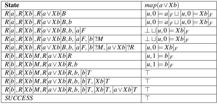
The following table reports a simple example of an evolution of a RuleRunner step and the corresponding value computed bymap. Let the property bea∨X band the trace beu= [b−b]. The index is incremented when the reactivation rules are fired.
State map(a∨X b)
R[a],R[X b],R[a∨X b]B [u,0|=a]Ft[u,0|=X b]F
R[a],R[X b],R[a∨X b]B,b [u,0|=a]Ft[u,0|=X b]F
R[a],R[X b],R[a∨X b]B,b,[a]F ⊥ t[u,0|=X b]F
R[a],R[X b],R[a∨X b]B,b,[a]F,[b]?M ⊥ t[u,0|=X b]F
R[a],R[X b],R[a∨X b]B,b,[a]F,[b]?M,[a∨X b]?R [u,0|=X b]F
R[b],R[X b]M,R[a∨X b]R [u,1|=b]F
R[b],R[X b]M,R[a∨X b]R,b [u,1|=b]F
R[b],R[X b]M,R[a∨X b]R,b,[b]T > R[b],R[X b]M,R[a∨X b]R,b,[b]T,[X b]T > R[b],R[X b]M,R[a∨X b]R,b,[b]T,[X b]T,[a∨X b]T >
[image:11.612.125.483.69.244.2]SUCCESS >
Table 2: Themapfunction
[u,0|=φ]F such that map(φ) =rj. In other words, RuleRunner’s state can always be mapped onto an
FLTL judgement overφ.
Proof 1 The proof proceeds by induction onφ:
• φ=a
If the formula is a simple observation, then the initial state is R[a], and map(R[a]) = [u,0|=a]F.
Adding observation to the state does not change the resulting FLTL judgement. If a is observed, RuleRunner will add[a]T to the state, and this will be mapped to>. If a is not observed, RuleRunner will add[a]F to the state, and this will be mapped to⊥. So for this simple case, the evolution of RuleRunner’s state corresponds either to the rewriting[u,0|=a]F=>(if a is observed) or to the
rewriting[u,0|=a]F=⊥(if a is not observed).
• φ=!a
This case is analogous tho the previous one, with opposite verdicts.
• φ=ψ1∨ψ2
By inductive hypothesis, a RuleRunner system monitoringψ1always corresponds to a rewriting of[u,i|=ψ1]. The same holds for ψ2. Let hRiR,RiE,Sii be RuleRunner system monitoring the subformulaψ1, with i∈ {1,2}. A RuleRunner system encodingφ includes R1and R2rules and specific rules for ψ1∨ψ2 given the truth values of ψ1 and ψ2. The initial state is therefore R[ψ1∨ψ2]∪S1∪S2, and this is mapped to map(S1)tmap(S2). By inductive hypothesis, this is a valid FLTL judgement. In each iteration, as long as the truth value ofψ1∨ψ2 is not computed, the state is mapped on map(S1)tmap(S2). When the propagation of truth values reachesψ1∨ψ2, the assigned truth value mirrors the evaluation table for the disjunction. If eitherψ1orψ2is true, thenφis true, and map(φ) =>. This corresponds to the valid rewriting map(S1)tmap(S2) =>, given that we are considering the case in which there is a trueψi: [ψi]T belongs to the state and map(ψ1) =>. The false-false case is analogous. In the?B case, the mapping is preserved,
and this is justified by the fact that bothψ1andψ2are undecided in the current cell, therefore map(ψi)6=>,⊥, therefore map(ψ1)tmap(ψ2)could not be simplified. In the?Lcase, we have
this is a valid rewriting since map(ψ1)tmap(ψ2) =map(ψ1)t ⊥=map(ψ1). The ?R case is
symmetrical.
• φ=ψ1∧ψ2
Same as above, with the evaluation table for conjunction on the RuleRunner side and theuoperator on the FLTL judgement side.
• φ=Xψ
A RuleRunner system encoding Xφhas initial state R[Xφ], which is mapped on[u,0|=Xψ]F. Then,
if the current cell is the last one, R[Xφ]evaluates to[Xφ]F, and the corresponding FLTL judgement is⊥. If another cell exists, R[Xφ]evaluates to[Xφ]?(with the same mapping). When the reactivation rules are triggered,[Xφ]?is substituted by R[Xψ]M,R[ψ]. Over this state, map(Xψ) =map(ψ), and the index is incremented since reactivation rules were fired. Therefore, the FLTL rewriting is
[u,i|=Xψ] = [u,i+1|=ψ], and this is a valid rewriting.
• φ=Wψ
This case is like the previous, but if the current cell is the last then R[Wψ]evolves to[Wψ]T ; the mapping is rewritten from[u,i|=Wψ]to>, and this is a valid rewriting if there is no next cell.
• φ=ψ1Uψ2
The initial RuleRunner system includes rules for ψ1, ψ2 and for the U operator. As long as R[ψ1Uψ2]A is not evalued, map(ψ1Uψ2) =map(ψ2)t(map(ψ1)u(map(X(ψ1Uψ2)))), that is, the standard one-step unfolding of the ’until’ operator as defined in FLTL. When a truth value for the global property is computed, there are several possibilities. The first one is that ψ2 is true andψ1Uψ2 is immediately satisfied. RuleRunner adds [ψ1Uψ2]T to the state and map(φ) =>; this corresponds to the rewriting map(ψ2)t(map(ψ1)u(map(X(ψ1Uψ2)))) =
> t(map(ψ1)u(map(X(ψ1Uψ2)))) =>, which is a valid rewriting. The case for[ψ1]F and
[ψ2]F is analogous. The?A case means that the evaluation for the until is undecided in the current
trace, and is mapped on the standard one-step unfolding of the until operator in FLTL. The?B
case implicitly encode the information that ’the until cannot be trivially satisfied anymore’, and henceforth the FLTL mapping is map(ψ1)u(map(X(ψ1Uψ2))). The cases for?Land?R have
the exact meaning they had in the disjunction and conjunction cases. For instance, if[ψ1]F and
[ψ2]?, RuleRunner adds[ψ1Uψ2]?R to the state, and for the obtained state map(φ) =map(ψ2). The sequence of FLTL rewriting is map(ψ2)t(map(ψ1)u(map(X(ψ1Uψ2)))) =map(ψ2)t(⊥
u(map(X(ψ1Uψ2)))) =map(ψ2)t ⊥=map(ψ2). Corollary 1 RuleRunner yields a FLTL verdict.
Proof 2 RuleRunner is always in a state that can be mapped on a valid FLTL judgement; therefore, when a binary truth evaluation for the encoded formula is given, this is mapped on the correct binary evaluation in FLTL. But since for such trivial case the map function corresponds to an identity, the RuleRunner evaluation is a valid FLTL judgement. The fact that RuleRunner yields a binary verdict is guaranteed provided that the analysed trace is finite, thanks to end-of-trace rules.
4
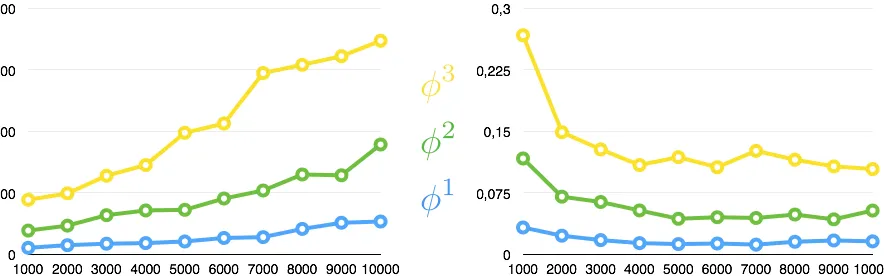
Experiments
φ1,2,3in three RuleRunner systems and used them to monitor traces randomly generated using the Latin alphabet as set of observations. Note that each monitoring process can terminate before the end of the trace (e.g. trivially, ifais observed while monitoring♦a); we measured the time required to actually monitor a given number of cells.
1
2
[image:13.612.87.529.142.280.2]3
Figure 2: Absolute (left) and averaged (right) performance of monitors encodingφ1,2,3
Figure 2 shows the time required, for the three rule systems, to monitor an increasing number of cells. In both subfigures, the x-axis represent the number of monitored cells and the y-axis a time measurement in milliseconds (ms). The three curves, in both subfigures, correspond to the three monitors forφ1=♦a,φ2=((a∨b)∨(c∨d))andφ3=♦((a∧X b)∨(c∧W d)). Figure 2(A) reports total times and Figure 2(B) reports average monitoring time per cell. The trends show how the monitoring time scales w.r.t. the number of the traces; the decreasing of average times in the curves of Figure 2(B) is due to the overhead to compute the rule system becoming less relevant when averaging with a larger number of cells. These experiment can be replicated with the tool available at www.di.unito.it/∼perotti/RuleRunner.jnlp.
5
Conclusions and Future Work
In this paper we present RuleRunner, a rule-based runtime verification system that exploits Horn clauses in implication form and forward chaining to perform a monitoring task. RuleRunner is a module in a wider framework that includes the encoding of the rule system in a neural network, the exploitation of GPUs to improve monitoring performances (as computation in neural networks boils down to matrix-based operations) and the adoption of machine learning algorithms to adapt the encoded property to the observed trace. Our final goal is the development of a system for scalable and parallel monitoring and capable to provide a description of patterns that falsified the prescribed temporal property. The applications of this frameworks spans from multi-agent systems (where a system designer may want to use an agent’s unscripted solution to a problem as a benchmark for all other agents [9]) to security (where a security manager may want to correct some false positives when monitoring security properties [5]).
6
Bibliography
References
[1] Wil M. P. van der Aalst et.al.: Process Mining Manifesto. In: Procs of Business Process
Management Workshops 2011, pp. 169–194. Available at http://dx.doi.org/10.1007/
978-3-642-28108-2_19.
[2] Howard Barringer, David E. Rydeheard & Klaus Havelund (2010):Rule Systems for Run-time Monitoring: from Eagle to RuleR. Journal of Logic and Computation volume 20, pp. pages 675–706. Available at
http://dx.doi.org/10.1093/logcom/exn076.
[3] Andreas Bauer, Martin Leucker & Christian Schallhart: The Good, the Bad, and the Ugly, But How Ugly Is Ugly? In:Procs. of Runtime Verification 2007, pp. 126–138. Available athttp://dx.doi.org/10.
1007/978-3-540-77395-5_11.
[4] Andreas Bauer, Martin Leucker & Christian Schallhart:Monitoring of Real-Time Properties. In:Procs. of Foundations of Software Technology and Theoretical Computer Science 2006, pp. 260–272. Available at
http://dx.doi.org/10.1007/11944836_25.
[5] David Breitgand, Maayan Goldstein & E. H. Shehory (2011):Efficient Control of False Negative and False Positive Errors with Separate Adaptive Thresholds.Network and Service Management, IEEE Transactions on
8, pp. 128–140. Available athttp://dx.doi.org/10.1109/TNSM.2011.020111.00055.
[6] Doron Drusinsky:The Temporal Rover and the ATG Rover. In:Procs. of the International Workshop on SPIN Model Checking and Software Verification 2000, pp. 323–330. Available athttp://dx.doi.org/10.
1007/10722468_19.
[7] Cindy Eisner, Dana Fisman, John Havlicek, Yoad Lustig, Anthony McIsaac & David Van Campenhout:
Reasoning with Temporal Logic on Truncated Paths. In:Procs. of Computer-Aided Verification 2003, pp. 27–39. Available athttp://dx.doi.org/10.1007/978-3-540-45069-6_3.
[8] Artur S. d’Avila Garcez & Gerson Zaverucha (1999): The Connectionist Inductive Learning and Logic Programming System. Applied Intelligencevolume 11, pp. pages 59–77. Available athttp://dx.doi.
org/10.1023/A:1008328630915.
[9] Christopher D. Hollander & Annie S. Wu (2011):The Current State of Normative Agent-Based Systems.J. Artificial Societies and Social Simulation14, pp. 47–62. Available athttp://jasss.soc.surrey.ac.
uk/14/2/6.html.
[10] Alfred Horn (1951):On Sentences Which are True of Direct Unions of Algebras.J. Symb. Log.16, pp. 14–21. Available athttp://dx.doi.org/10.2307/2268661.
[11] Saul A. Kripke (1963):Semantical Considerations on Modal Logic.Acta Philosophica Fennica16, pp. 83–94. [12] Jean-Louis Lassez & Michael J. Maher:The Denotational Semantics of Horn Clauses as a Production System.
In:Procs. of the Association for the Advancement of Artificial Intelligence 1983, pp. 229–231. Available at
http://www.aaai.org/Library/AAAI/1983/aaai83-006.php.
[13] Martin Leucker & Christian Schallhart (2009):A brief account of runtime verification.Journal of Logic and Algebraic Programmingvolume 78, pp. pages 293–303. Available athttp://dx.doi.org/10.1016/
j.jlap.2008.08.004.
[14] Orna Lichtenstein, Amir Pnueli & Lenore D. Zuck:The Glory of the Past. In:in Procs. of Logic of Programs 1985, pp. 196–218. Available athttp://dx.doi.org/10.1007/3-540-15648-8_16.
[16] Amir Pnueli: The temporal logic of programs. In: Procs. of the Annual Symposium on Foundations of Computer Science 1977, pp. 46–57. Available athttp://doi.ieeecomputersociety.org/10.
1109/SFCS.1977.32.
[17] M. H. Van Emden & R. A. Kowalski (1976):The Semantics of Predicate Logic As a Programming Language.