City, University of London Institutional Repository
Citation
:
Miessi Sanches, F.A., Silva Junior, D. & Srisuma, S. (2016). Ordinary Least Squares Estimation of a Dynamic Game Model. International Economic Review, 57(2), pp. 623-634. doi: 10.1111/iere.12170This is the accepted version of the paper.
This version of the publication may differ from the final published
version.
Permanent repository link: http://openaccess.city.ac.uk/16624/
Link to published version
:
http://dx.doi.org/10.1111/iere.12170Copyright and reuse:
City Research Online aims to make research
outputs of City, University of London available to a wider audience.
Copyright and Moral Rights remain with the author(s) and/or copyright
holders. URLs from City Research Online may be freely distributed and
linked to.
City Research Online: http://openaccess.city.ac.uk/ [email protected]
Ordinary Least Squares Estimation
of a Dynamic Game Model
Fabio A. Miessi Sanches
yUniversity of São Paulo
Daniel Silva Junior
zLondon School of Economics
Sorawoot Srisuma
xUniversity of Surrey
July 28, 2014
Abstract
The estimation of dynamic games is known to be a numerically challenging task. In this paper we propose an alternative class of asymptotic least squares estimators to Pesendorfer and Schmidt-Dengler’s (2008), which includes several well known estimators in the literature as special cases. Our estimator can be substantially easier to compute. In the leading case with linear payo¤s speci…cation our estimator has a familiar OLS/GLS closed-form that does not require any optimization. When payo¤s have partially linear form, we propose a sequential esti-mator where the parameters in the nonlinear term can be estimated independently of the linear components, the latter can then be obtained in closed-form. We show the class of estimators we propose and Pesendorfer and Schmidt-Dengler’s are in fact asymptotically equivalent. Hence there is no theoretical cost in reducing the computational burden. Our estimator appears to perform well in a simple Monte Carlo experiment.
JEL Classification Numbers: C14, C25, C61
Keywords: Closed-form Estimation, Dynamic Discrete Choice, Markovian Games.
We are grateful to Martin Pesendorfer for encouragement and support. We thank Joachim Groeger, Oliver Linton, Robert Miller, Pasquale Schiraldi, Richard Smith and Dimitri Szerman for helpful advice and comments.
1
Introduction
We consider the estimation problem for a class of dynamic games of incomplete information that generalizes the single agent discrete Markov decision models surveyed in Rust (1994); for a recent survey see Aguirregabiria and Mira (2010). The setup is in an in…nite time horizon, where players’ private values enter the payo¤ function additively and are independent across players, under the conditional independence framework. A Markov equilibrium of such game can be represented by a …xed point of nonlinear equations in the space of choice probabilities and has been shown to exist (e.g. see Aguirregabiria and Mira (2007) and Pesendorfer and Schmidt-Dengler (2008)). A variety of methods have been proposed by di¤erent authors to estimate the same class of games based on the equilibrium condition in recent years; examples are given below. However, a common component of these methodologies is a nonlinear optimization problem that may act as a considerable deterrent for applied researchers to estimate dynamic games due to involved programming needs and/or long computational time.
In this paper we propose a class of asymptotic least squares estimators constructed based on the equilibrium condition of the game when represented in the space of payo¤s. Our work is motivated by the well-received methodology developed in Pesendorfer and Schmidt-Dengler (2008), who propose an e¢ cient estimator for a unifying class of estimators that includes the non-iterative pseudo-likelihood estimator of Aguirregabiria and Mira (2007) and the moment based estimators discussed in Pakes, Ostrovsky and Berry (2007) as special cases. In contrast to our work, Pesendorfer and Schmidt-Dengler use the choice probability representation of the equilibrium to construct their estimator. Our goal is to show there is much to gain computationally using our approach with no e¢ ciency lost. Henceforth we use the abbreviation ALSEP SD when referring to a generic estimator of Pesendorfer and Schmidt-Dengler.
We claim our estimator can be substantially easier to compute than ALSEP SD. In the leading case our estimator has a familiar OLS/GLS closed-form expression when the per-period payo¤ function takes a linear-in-parameter speci…cation.1 In an intermediate case when the payo¤ function has an
additive partially linear form, Frisch-Waugh-Lovell theorem can be applied so the parameters in the nonlinear part can be estimated …rst (dimensional reduction), and the linear-in-parameter component
1The linear payo¤s structure may seem restrictive, but it is in fact quite general as it includes any nonlinear (basis)
can be obtained in closed-form in the second step.2 Even in a more general nonlinear case, we argue
that our estimator is still generally easier to compute than ALSEP SD. ALSEP SDalso provides a good benchmark for a comparison with other estimators in the literature as it has a well-de…ned e¢ ciency property. We establish a duality between our estimator and ALSEP SD, in the sense that they can always be constructed to have the same asymptotic distribution. Therefore our e¢ cient estimator is as e¢ cient as the e¢ cient ALSEP SD.
The large sample properties of our estimator (and for asymptotic least squares generally) are easy to derive for discrete games. Technically, our estimation problem is a least squares problem with generated regressors and regressands, which are generally smooth functions of the …nite dimensional …rst stage parameters that are nonparametrically identi…ed. In addition, the number of square terms in the objective function does not grow with sample size but is determined by the cardinality of the action and state spaces. Therefore our estimator belongs to the class of asymptotic least squares estimators as de…ned in Gourieroux and Monfort (1985,1995) in the same sense as ALSEP SD. The close connection between our estimator and ALSEP SD goes even further given the smooth bijective relation between normalized expected payo¤s and choice probabilities (Hotz and Miller (1993)’s inversion); ALSEP SD is de…ned to minimize the distance between the probabilities implied by the pseudo-model and the data. We show that, locally around the true, using the inverse function theorem, our estimator can be constructed to have the same asymptotic distribution as any ALSEP SD by choosing an appropriate weighting matrix and vice versa.
There are at least two reasons why the estimation of dynamic games can be non-trivial. First, as well-known from the single-agent problem, it involves value functions that generally do not have closed-form and need to be numerically evaluated so it is computationally demanding (see Rust (1996)). For games, there is also a potential issue of indeterminacy of multiple equilibria that gives rise to incomplete models (Tamer (2003)). A novel approach popularized by Hotz and Miller (1993) performs inference on the pseudo-model, generated from to the observed data, by estimating the (policy) value functions that can signi…cantly simplify the computational aspect. Pseudo-models are also generally easier to handle in a strategic environment as they have been shown to be complete for several classes of games (Srisuma (2013b)). Methodologies based on pseudo-models are often referred to as two-step estimators since they require estimation of value functions in the …rst stage. Many recently proposed estimators for dynamic games are two-step estimators.
However, despite the simpli…cation of two-step methods, the numerical aspects for implementing existing estimators in the literature appear to remain a concern as they generally involve solving highly nonlinear optimization problems. It is not uncommon to see methodology papers using
esti-2Modeling of additive linear components in the payo¤s often appear in games with entry/exit decisions, as …xed
mation time, amongst other things, as a competing factor. Furthermore, it is also not unusual that the choice of players’per-period payo¤ speci…cation is chosen with the ease of numerical implemen-tation in mind. In particular there can be substantial bene…ts (in terms of compuimplemen-tational time) in specifying player’s payo¤ functions to be linear-in-parameters. As the action-speci…c expected payo¤s can then be written as a linear transformation of the parameter, following from the linear structure that de…nes the expected payo¤s using stationary Markovian beliefs; examples of such discussions can be found in Bajari, Benkard and Levin (2007, Section 3.3.1) and Pakes, Ostrovsky, Berry (2007, Section 3). As a result, a linear parameterization of the payo¤s is a leading speci…cation employed in empirical work (see Footnote 1 for examples).
The objective functions that are used to de…ne many two-step estimators in the literature are constructed in terms of choice probabilities implied by the pseudo-model. These probabilities can be motivated by the equilibrium condition of the game, which can be stated in terms of consis-tent beliefs with probabilities of best responses. Choice probabilities are used to de…ne traditional criterion functions such as pseudo-likelihood function (Aguirregabiria and Mira (2007), Kasahara and Shimotsu (2012)) or moment and minimum distance based conditions (Pakes, Ostrovsky, Berry (2007), Pesendorfer and Schmidt-Dengler (2008)). However, in order to calculate the probabilities implied by the pseudo-model, one must …rst compute the expected discounted payo¤s that determine the region of integration to be integrated to compute the probabilities. Furthermore, the integral is generally a nonlinear map of the expected payo¤s, and it typically has to be computed numeri-cally outside the well-known conditional logit framework. The integral, following Hotz and Miller (1993)’s inversion result, in fact represents a one-to-one mapping between the probabilities and the normalized expected payo¤s.
an e¢ cient one-step estimator.3 ,4
The rest of the paper is organized as follows. Section 2 begins with an illustrative example that motivates our estimator, and then describes the model and our estimator for games. Section 3 gives the main results. Section 4 presents results from Monte Carlo experiments that compare the statistical performance and relative speed of our estimator and ALSEP SD. Section 5 concludes and provides a brief discussion on how our estimators can be adapted or applied to complement other recent results in the literature. All proofs can be found in the Appendix.
2
Methodology
We begin with an illustration that highlights the idea behind computational advantages of our esti-mation approach. Section 2.2 describes elements of the game. We de…ne the pseudo-model in Section 2.3 and introduce our estimator in Section 2.4.
2.1
Least Squares in Probabilities vs Payo¤s
Consider a model generated by the following binary choice variable:
at( ) =1[v (xt) "t] for 2 Rp;
where xt and "t are independent. Let the cdf of "t be denoted by Q. For all x, let P (x) =
Pr [at( ) = 1jxt =x], so that P (x) = Q(v (x)). Assume the support of xt is …nite, say fxjg
J j=1
for some J < 1, so that we can de…ne P = (v ), where P = (P (x1); : : : ; P xJ )>, v =
(v (x1); : : : ; v xJ )> and (v ) = (Q(v (x1)); : : : ; Q v xJ )>.
Suppose: we observe a random sample offat; xtgwhereat =at( 0)for some 0 2 , which is the
parameter value of interest; v is nonparametrically identi…ed up to , and there exists a consistent estimator of v , say vb , for all ; and,Q is known and invertible. LetP= (P(x1); : : : ; P xJ )> be a vector of choice probabilities identi…ed from the data, so that P=P 0, then one may consider a class of estimators de…ned by
bp(V) = arg min
2 Pe Pb >
V Pe Pb ; (1)
where Pe and Pb are estimators for P and P respectively, and V be some positive de…nite matrix. Note thatPe andPb 0 are generally di¤erent since the former is model-free while the latter is estimated
3An earlier version of Bajari et al. (2009), Bajari and Hong (2006), proposes a two-step estimator that can be seen
as the dynamic game version of Hotz et al. (1994).
4Another notable estimator that does not take a two-step approach is Egesdal, Lai and Su (2012). However, Egesdal
through vb . Similarly, we can de…ne v = (Q 1(P (x1)); : : : ; Q 1(P xJ ))>, which is also identi…ed
from the data, so that v=v 0 by construction. Then one can also consider an alternative class of
estimators:
bv(W) = arg min
2 (ev bv ) >
W(ev vb ); (2)
where ve is 1(P)e and
W is a positive de…nite matrix. As described previously,ve and vb 0 will also generally di¤er.
Equations (1) and (2) provide two di¤erent estimators for 0. We argue the latter should generally
be easier to compute than the former since it is more convenient to compute (ev;vb ) relative(Pe;Pb )
across di¤erent values of . This argument is most transparent when v has a linear-in-parameter speci…cation, i.e. v (xt) = >v(xt) for some p dimensional vector v(xt). Then vb can be written as Xb , where Xb is a J by p matrix such that its j th row equals bv(xj)>. The solution to (2) is unique and has a closed-form, Xb>WXb 1Xb>Wvb, when Xb>WXb is invertible. Even without the
linear parameterization of v , every evaluation of Pb requires the mapping of v (xj) by Q for all j, for every , where Q is generally a nonlinear function that may have to be computed numerically. In contrast, for (2), the potentially costly step of applying Q 1 has to be performed only once to
estimatevthat does not depend on . Regardless of the parameterization inv , under some suitable regularity conditions, and appropriate choices of weighting matrices, the two estimators can be shown to be asymptotically equivalent near 0 in the sense that there existsWV and VW such that for any
V and W:
p
N bv(WV) 0 = p
N bp(V) 0 +op(1);
p
N bp(VW) 0 = p
N bv(W) 0 +op(1); where N denotes the sample size.
The estimator in (1) is closely related to ALSEP SD and other Hotz and Miller (1993)’s type estimators that have been widely adopted in the dynamic game setting. In contrast the estimator based on (2) is the asymptotic least squares analog to the estimator proposed in Hotz et al. (1994). For the remainder of this section we develop an estimator based on (2) in the context of a dynamic game.
2.2
Framework
We consider a game withI players, indexed byi2 I =f1; : : : ; Ig, over an in…nite time horizon. The elements of the game in each period are as follows:
ait. Let at = (a1t; : : : ; aIt) 2 A = Ii=1A. We will also occasionally abuse the notation and write at = (ait;a it) where a it = (a1t; : : : ; ai 1t; ai+1t: : : ; aIt)2AnA.
States. Player i’s information set is represented by the state variables sit 2 S, where sit =
(xit; "it) such that xit 2 X is common knowledge to all players and "it 2 E =RK+1 denotes private information only observed by player i. Note that common state space X is without any loss of generality. We shall use sit and (xt; "it) interchangeably. We de…ne (st;s it;"t;" it;E) analogously to (at;a it; A), and denote the support of st byS =X E.
State Transition. Future states are uncertain. Players’actions and states today a¤ect future states. The evolution of the states is summarize by a Markov transition law P(st+1jst;at).
Per Period Payoff Functions. Each player has a payo¤ function, ui :A S !R, which is time separable. The payo¤ function for player ican depend generally on(at; xt; "it) but not directly on " it.
Discounting Factor. Future period’s payo¤s are discounted at the rate i 2 (0;1) for each player. For notational simplicity we take i = for all i.
We impose the following assumptions throughout the paper.
Assumption M1(Additive Separability). ui; i(ai;a i; x; "i) = i; i(ai;a i; x)+
P
a02A"i(a0)1[ai =a0]
for all i; i; ai;a i; x; "i, where i; i is known up to i 2 i R
pi.
Assumption M2 (Conditional independence). The transitional distribution of the states has the following factorization: P (xt+1;"t+1jxt;"t;at) = Q("t+1)G(xt+1jxt;at), where Q is the cumulative
distribution function of "t and G denotes the transition law of xt+1 conditioning on at and xt.
Assumption M3 (Independent private values). The private information is independently dis-tributed across players, and each is absolutely continuous with respect to the Lebesgue measure whose density is bounded on RK+1. So that Q(") =QI
i=1Qi("i), where Qi denotes the cumulative
distrib-ution function of "it.
Assumption M4 (Discrete public values). The support of xt is …nite so that X = x1; : : : ; xJ
for some J <1.
not essential for the general idea behind estimation of dynamic games. Although the complexity of the asymptotic theory and the practical aspects increase signi…cantly when xt includes continuous random variables; see Bajari et al. (2009) and Srisuma and Linton (2012).
At timetevery player observessit, each then choosesaitsimultaneously. We consider a Markovian framework where players’behaviors are stationary across time and players are assumed to play pure strategies. More speci…cally, for some i : S ! A, ait = i(sit) for all i; t, so that whenever
sit=si then i(sit) = i(si )for any . The beliefs are also time invariant. Playeri0s beliefs, i, is a distribution of at= ( 1(s1t); : : : ; I(sIt)) conditional onxt for some pure Markov strategy pro…le
( 1; : : : ; I). The decision problem for each player is to solve
max
ai2Aif
E i[ui; i(ait;a it; si)jsit = si; ait=ai] + E i[Wi; i(sit+1; i)jsit =si; ait =ai]g; (3)
where Wi; i(si; i) = 1
X
=t t
E i[ui; i(a ; si )jsit=si];
for any si. The subscript i on the expectation operator makes explicit that present and future actions are integrated out with respect to the beliefs i; in particular, player i forms an expectation for all players’future actions including herself, and todays actions of opposing players. Wi; i( ; i)is
a policy value function since the expected discounted return needs not be an optimal value from an optimization problem since i can be any beliefs, not necessarily equilibrium beliefs. Note that the transition laws for future states are completely determined by the primitives and the beliefs. Any strategy pro…le that solves the decision problems for all i and is consistent with the beliefs satis…es is an equilibrium strategy. It is well-known that players’best responses are pure strategies almost surely and Markov perfect equilibria for games under M1 - M4 (e.g. see Aguirregabiria and Mira (2007) and Pesendorfer and Schmidt-Dengler (2008)). However, there may be multiple equilibria.
2.3
Pseudo-Model
We now de…ne the pseudo-model that plays a central role in two-step estimation methods. The start-ing point is the structural assumption that we observe random sample off 1(s1t); : : : ; I(sIt); xt; xt+1g
from a single equilibrium, where i = i; i0 for some i0 2 i R
pi for all i. Let P
i (aijx) =
Pr [ i (sit) = aijxt=x] for allai; x. Then we have: (i) the equilibrium beliefs for all players is sum-marized byQIi=1Pi ; (ii)Pr [ait =aijxt=x] =Pi (aijx)andPr [xt+1 =x0jxt =x; at =a] =G(x0jx; a) for all a; x; x0. For notational simplicity, for this section and the next, we shall: omit ; let
i and
conditional distributions indexed by = ( >1; : : : ; >I)> 2 I
i=1 i = Rp. Also let 0 denote ( >10; : : : ; >I0)>.
Definition: The pseudo-model isfP g 2 such that P =QiI=1Pi; i and for alli; i; ai; x:
Pi; i(ajx) = Pr [ i; i(sit) =ajxt =x] a.s.; where
i; i(sit) = arg max
ai2Af
E[ i; i(ai; a it; xt)jxt] +"it(ai) + E[Vi; i(st+1)jxt; ait =ai]g;
Vi; i(sit) = E[ i; i(ait; a it; xt) +
K
X
a0=0
"it(a0)1[ait=a0]jsit] + E[Vi; i(sit+1)jsit]:
By construction Pi; i =Pi for all i when i = i0 for all i, and Vi; i also equalsWi; i( ; i)(as
de-…ned in (3)), when i =QIj=1Pj. Letvi; i(ai; x) =E[ i; i(ai; a it; xt)jxt=x]+ E[Vi; i(st+1)jxt =x; ait =ai],
then we can write
Pi; i(ajx) = Pr [vi; i(ai; xt) +"it(ai)> vi; i(a
0
i; xt) +"it(a0i) for all a0i 6=aijxt =x]; (4) which is familiar from the classical random utility model (e.g. see McFadden (1974)) with mean utility vi; i. The numerical advantage in working with the pseudo-model, as opposed to the actual
model, is that vi; i is relatively straightforward to compute for di¤erent i, since all expectations that
de…ne vi; i are calculated independent of i; all with respect to P (st+1jst; at) for all players that is
equivalent to earlier notation using E i when i =
QI
j=1Pj for all i.
We shall heavily exploit the fact thatvi; i is a linear transformation of i; i. To see this, …rst look
at the choice-speci…c expected return:
E[Vi; i(st+1)jxt; ait =ai] = E[E[Vi; i(st+1)jxt+1]jxt; ait =ai]; and
E[Vi; i(st)jxt] = E[ i; i(ait; a it; xt) +
K
X
a0=0
"it(a0)1[ait =a0]jxt] + E[E[V i(st+1)jxt+1]jxt]:
Let mi; i = E[Vi; i(sit)jxt = ] and gi; i = E[Vi; i(sit+1)jxt = ; ait = ]. Then, using a linear
functional notation, we have
gi; i = Himi; i;
mi; i = ri; i+ri+Lmi; i; where for all a; x
ri; i(x) = E[ i; i(ait; a it; xt)jxt=x];
ri(x) = E[
K
X
a0=0
"it(a0)1[ait=a0]jxt=x];
Lm(x) = E[m(xt+1)jxt=x];
where L and Hi are linear maps and ri; i is a linear transformation of i; i. Since (I L)
1
is also generally a well-de…ned linear map, as L is a contraction as its norm is strictly less than 1, then
vi; i = Ri+ Hi(I L)
1
R i; i +vi;
where Ri and Rare conditional expectation operators, conditioning onxt, integrating overa it and
at respectively , andvi = Hi(I L) 1ri.
The choice probabilities can also be written in terms of di¤erences in choice speci…c expected payo¤s. Let vi; i(ai; x) denotevi; i(ai; x) vi; i(0; x)for ai >0, then (4) becomes
Pi; i(ajx) = Pr [ vi; i(ai; xt) +"it(ai)> vi; i(a
0
i; xt) +"it(a0i) for all a0i >0jxt =x]: (5) Since A and X are …nite, the relationship between f vi; i(ai; x)gai>0;x2X and f i; i(a; x)ga2A;x2X
can be represented through a matrix equation. We state this representation as a lemma.
Lemma R: Under M1 - M4 f vi; i(ai; x)gai>0;x2X can then be represented by a J K vector,
vi; i:
vi; i =D(Ri+ HiMR) i; i+ vi; (6) where i; i is a J(K+ 1)
I
vector of f i; i(a; x)ga2A;x2X so that elements in: Ri i; i are
fE[ i; i(ai; a it; xt)jxt=x]gai2A;x2X; R i; i are fE[ i; i(ait; a it; xt)jxt=x]gx2X; M involve
fPr [xt+1 =x0jxt =x]g; Hi are Pr [xt+1 =x0jxt=x; ait=ai]; and, D is a di¤erence matrix with re-spect to the expected payo¤s from playing action 0; and, vi is the di¤erenced vector form of the transformation of ri by iHi(I L)
1
normalized by action 0. The detailed constructions of
vi;D;Ri;R;Hi and M are provided in the Appendix.
In what follows, we let vi denote vi; i0. And, similarly, it shall be convenient to
vector-ize the probabilities. In particular, we let Pi; i and Pi denote the J K vector that represent
fPi; i(aijx)gai>0;x2X and fPi(aijx)gai>0;x2X respectively.
2.4
Estimation
Many objective functions proposed in the literature often can be written directly in terms of the probabilities from the pseudo-model, such as pseudo-likelihood and GMM, based on the construction that Pi; i coincides with Pi when i = i0. However, from a numerical perspective, computing the
pseudo-probabilities requires a costly additional step of computation, namely the integration with respect to the distribution of"it that maps vi; i intoPi; i (see (5)). These integrals generally do not
mapping of vi; i intoPi; i. In order to preserve the linear structure outlined previously, we propose
to construct objective functions based directly on vi; i.
The validity of such objective functions, to identify 0, follows from the bijective relation between vi; i and Pi; i for each i. This well-known result follows from Proposition 1 of Hotz and Miller
(1993), which we shall refer to as Hotz and Miller’s inversion in this paper (also see Lemma 8 of Matzkin (1991), Lemma 1 of Pesendorfer and Schmidt-Dengler (2008), and, for a recent generalization of these results, Norets and Takahashi (2013)).5 In particular, it immediately follows that for any
i,Pi; i coincides withPi if and only if vi; i coincides with vi, where vi is identi…able from the
data by Hotz and Miller’s inversion. Then we can construct a class of estimators based on minimizing the distance between f vi; ig
I
i=1 and f vig
I i=1.
Using Lemma R, we can write vi; i =Xi( i) + vi, where
Xi( i) = D(Ri+ HiMR) i; i: (7)
Note that i enters Xi( i) through a matrix transform of the vector i; i, where the former does
not depend on i and the latter is completely known and speci…ed by the researcher. By Hotz and Miller’s inversion, we also have vi = i(Pi) for some nonlinear, but known, function i that only depends on the distributional assumption of "it. Then we can de…ne a J K vector, Yi, where
Yi = i(Pi) vi: (8)
Note that Yi is de…ned independently of i. So that, by construction:
Yi =Xi( i) when i = i0:
LetY = Y>
1 ; : : : ;YI>
>
, = >1; : : : ; >I >and de…ne a block diagonal matrixX ( ) =diag(X1( 1);
: : : ;XI( I)). In the next section we analyze the asymptotic properties for a class of estimators that are motivated from minimizing
S( ;W) = (Y X ( ))>W(Y X( )); (9)
over , for some weighting matrixW.
It is also worth emphasizing that, throughf vigIi=1;fRig I
i=1;R;Land fHig I
i=1, for any :X ( )
andY are explicit functions, sayTX( ; 0)andTY( 0)respectively, of a …nite-dimensional vector, 0,
that consists of choice and transition probabilities. However, optimization withS( ;W)is infeasible since X ( ) and Y are not observed, as 0 is unknown. Given a sample from a single equilibrium,
5Pesendorfer and Schmidt-Dengler (2008) also show equilibrium condition can be characterized in terms of expected
f 1(s1t); : : : ; I(sIt); xt; xt+1g, 0can be identi…ed from the data under weak conditions, henceX ( )
and Y can also be estimated directly from the data for all . Consequently we consider a feasible estimation criterion where X and Y are replaced by Xb( ) =TX ( ;b) and Yb = TY (b) respectively, for some preliminary estimator, b, of 0. We denote the sample counterpart of S bySb, so that
b
S( ;Wc) = (Yb Xb( ))>Wc(Yb Xb( )); (10)
where Wc can be random and depend on the sample size. We de…ne our estimator,b(Wc), to be the minimizer of Sb ;Wc :
b(Wc) = arg min
2 Sb( ;Wc):
Thereforeb(Wc) is generally a nonlinear least square estimator with generated regressors and regres-sands. Note that Sb( ;Wc) is easy to evaluate for di¤erent values of , following (7) and (8), Xbi( ) can be computed by a matrix multiplication of i; i by the estimator of D(Ri+ HiMR), which
does not depend on i, and Ybi is also independent of i.
3
Main Results
We give large sample properties of our estimator in full generality in Section 3.1. We consider special cases when payo¤s have linear-in-parameter and partially linear speci…cations in Section 3.2 and 3.3 respectively. We discuss the relationship between our estimator and ALSEP SD in Section 3.4. In what follows we denote the matrix norm by k k, so that kBk =ptrace(B>B) for any real matrix
B, and we let “!p ” and “!d” denote convergence in probability and distribution respectively.
3.1
General Case
From the previous section, we see that TX ( ; ) and TY( ) are deterministic and smooth functions in for any . To analyze the asymptotic properties ofb(Wc), it will be useful to keep separate the sampling distribution of the preliminary estimator and the corresponding generated regressors and regressands. We begin with a preliminary requirement for b.
Assumption P: (i) b!p 0; and, (ii) p
N(b 0)! Nd (0; ).
Assumption A1: 0 2 int( ) where is a compact subset of Rp, and X( ) = X( 0) if and
only if = 0.
Assumption A2: Wc! Wp , where W is a non-stochastic positive de…nite matrix.
Assumption A3: sup 2 kX( )k and kYk are …nite, and sup 2 Xb( ) X( ) !p 0 and
b
Y ! Yp .
Assumption A4: X( ) is continuously di¤erentiable at 0 and rX = @@X( )> = 0
has full column rank.
Assumption A5: sup 2B (
0)
@Xb( )
@ >
@X( )
@ >
p
!0, where B ( 0) denotes some neighborhood of 0.
De…neUb=Yb Xb( 0).
Assumption A6: pNUb! Nd (0; )for some non-stochastic positive de…nite matrix .
Comments on Assumptions A1 - A3.
These conditions are su¢ cient for the consistency of our estimator. A1 - A2 constitute to a high level identi…cation condition as it ensures (9) has a unique solution at 0. There has been
little work on more primitive conditions for parametric identi…cation of payo¤ functions in dynamic games. Most identi…cation results in the literature are nonparametric that build on the work of Magnac and Thesmar (2002); see Pesendorfer and Schmidt-Dengler (2008) and Bajari et al. (2009). However, using Hotz and Miller’s inversion, it follows that the condition for identi…cation of the pseudo-model at 0, in the sense that Pi; i = Pi; i0 for all i if and only if i = i0 for all i, is
precisely the identi…cation condition required in A1. Furthermore, by inspecting Lemma R more closely, for each i, we see that the necessary and su¢ cient condition for the unique parameterization of Xi( i) at i0 is for the intersection between the f i; i i; i0 : i 2 in f i0gg and the null
space of D(Ri+ HiMR) to be empty. Although, without any restriction on i; i, A1 generally
does not hold since D(Ri+ HiMR) is always rank-de…cient. For a closely related discussion see Srisuma (2013a), who provides constructive conditions for parametric identi…cation results in a single agent model that can be generalized directly to the games considered in this paper. Also see the identi…cation condition and comments of B1 in Section 3.2 when linear-in-parameter restriction is imposed. The uniform boundedness and consistency conditions essentially depend on f i; ig
I i=1. In
particular, if D(Ri+ HiMR)is …nite then continuity of f i; ig
I
i=1 ensuressup 2 kX ( )kis …nite
since is compact. Then uniform consistency also follows if there exists a consistent estimator for
Comments on Assumptions A4 - A6.
For the distribution theory, additional local conditions around 0 are required. A4 - A5 are
standard smoothness and regularity conditions for an asymptotic normality of an extremum estimator that optimizes a smooth objective function. Similar to the discussion of su¢ cient conditions for A3, using Lemma R, a su¢ cient condition for continuous di¤erentiability of X( ) in A4 is continuous di¤erentiability of i; i at i0 for all i, then A5 will also follow if P(i) holds. Furthermore, if P(ii)
holds, so that the elements inXb( 0)andYbhave asymptotically normal distribution, then by applying
a delta-method A6 also holds with =r r>, where r = @
@ >(TY( ) TX ( 0; ))j = 0.
Our estimators are consistent and asymptotically normal under these assumptions.
Theorem 1 (Consistency): Under assumptions A1 - A3, b(Wc)!p 0.
Theorem 2 (Asymptotic Normality): Under assumptions A1 - A6,
p
N b(Wc) 0
d
! N(0; W);
where W = r>XWrX 1r>XW WrX r>XWrX 1.
In large sample, the estimators that uniquely solve (10) are distinguishable up to the …rst order by W. The e¢ cient estimator in this class can be found by choosing the optimal weighting matrix,
W , that minimizes W over the set of all possible positive de…nite matrices (i.e. e¢ ciency gain in the spirit of Chamberlain (1982) and Hansen (1982) for instance).
Theorem 3 (Efficiency): Under assumptions A1 - A6, (i) the asymptotic variance of pN b(Wc) 0
is bounded below by 1 = r>
X 1rX
1
; and, (ii) if Wc !p 1 then pN b(c
W) 0
d
! N (0; 1).
The …rst part of Theorem 3 says that the lower variance bound for the class of estimators we consider is r>X 1rX 1. The second part states that any consistent estimator of 1 is su¢ cient to produce an e¢ cient estimator. In practice, consistent estimator for 1 will typically require a
preliminary consistent estimator for 0. The simplest choice is to chooseW to be an identity matrix,
Id. In this case the estimator for i0 can be computed individually for each player. We state this in
the following corollary.
Corollary A (Identity Weighted Estimator): Under assumptions A1, A3 - A6,
p
N b(Id) 0
d
! N (0; Id), where b(Id) = b1(Id)>; : : : ;bI(Id)> >
. Furthermore, for all i:
bi(Id) = arg min i2 i(Ybi Xbi( i))>(Ybi Xbi( i)) such that
p
N bi(Id) i0
d
! N(0; r>XirXi
1
r>Xi irXi r > XirXi
1
) with rXi =
@Xi( )
@ >
i i= i0
and i = limN!1V ar(
p
3.2
Linear-in-Parameter Speci…cation
We now consider the leading special case when payo¤ functions have a linear-in-parameter speci…ca-tion.
Assumption M5 (Linear-in-parameter payo¤s). For all (i; i; ai; a i; x),
i; i(ai; a i; x) = >
i i(ai; a i; x);
for some p dimensional vector i(ai; a i; x) = ( 1i (ai; a i; x); : : : ; pi (ai; a i; x))>.
We assume M1 - M5 hold throughout this subsection. Then, with a slight abuse of notation,
Xi( i) in (7) simpli…es toXi i, where
Xi =D(Ri+ HiMR) i; (11)
and i is a J(K+ 1) I
by p matrix of f i(ai; a i; x)gai2A;x2X. Let X = diag(X1; : : : ;XI). The
limiting and sample objective functions de…ned in (9) and (10) respectively become
Slip( ;W) = (Y X )>W(Y X ); and
b
Slip( ;Wc) = (Yb Xb )>Wc(Yb Xb ):
IfXb>WcXbis non-singular, thenSblip( ;Wc)is globally convex. The solution to the minization problem has a well-known closed-form expression of a weighted least squares estimator, namely
blip
(Wc) = Xb>WcXb 1Xb>WcYb: (12)
Although the large sample properties for blip(Wc) follow immediately from Section 3.1, they can be specialized substantially to incorporate M5. Since the results in this subsection may be most relevant for empirical applications we provide some details here.
Assumption B1: X has full column rank.
Assumption B2: Wc! Wp , where W is a non-stochastic positive de…nite matrix.
Assumption B3: kX k and kYk are …nite, and Xb! Xp and Yb! Yp . De…neUblip = b
Y Xb 0.
Assumption B4: pNUblip d
! N 0; lip for some non-stochastic positive de…nite matrix lip.
Similar to A1 - A2, B1 and B2 ensureSlip( ;
W)has a unique solution at 0. In this case, the full
rank condition of X is a necessary and su¢ cient condition for the identi…cation of the pseudo-model (for more details see Srisuma (2013)). The sample counterpart of B1, namely the rank condition of
b
X, also has a …nite sample signi…cance. IfWcis positive de…nite, then the full column rank condition of Xb is necessary and su¢ cient for Sblip( ;c
W) to have a unique solution, which equals to blip(Wc) as de…ned in (12). Assumptions B3 and B4 are immediate specializations of A3 - A6.
We state the large sample properties forblip(Wc) as corollaries without proofs.
Corollary 1 (Consistency): Under assumptions B1 - B3, blip(Wc)!p 0.
Corollary 2 (Asymptotic Normality): Under assumptions B1 - B4,
p
N blip(Wc) 0
d
! N 0; lipW ;
where lipW = X>WX 1X>W lip
WX X>WX 1.
Corollary 3 (Efficiency): Under assumptions B1 -B4, (i) the asymptotic variance of pN blip(Wc) 0
is bounded below by liplip 1 = X
> lip 1
X 1
; and, (ii) if Wc!p lip 1 then pN blip(Wc) 0
d
!
N 0; liplip 1 .
Similarly to the general case, consistent estimator for lip 1 requires a preliminary consistent estimator for 0. We have the counterpart to Corollary A when we choose W to be an identity
matrix I.
Corollary B (Identity Weighted Estimator): Under assumptions B1, B3 and B4,
p
N blip(I) 0
d
! N 0; lipI , whereblip(I) = Xb>Xb 1Xb>Yband lip
I = X>X 1
X> X X>X 1:
Furthermore, for all i: blip(I) = blip1 (I)>; : : : ;blip
I (I)>
>
such that blipi (I) = Xb>
i Xbi
1
b
X>
i Ybi and
p
N blipi (I) i0
d
! N(0; Xi>Xi
1 Xi>
lip
i Xi Xi>Xi
1
) with lipi = limN!1V ar(
p
N(Ybi
b
Xi i0).
We have shown here that once we have (Yb;Xb), under some regularity conditions, a consistent estimator for 0 can be obtained by an OLS estimator, b
lip
(I) = Xb>Xb 1Xb>Yb (Corollary B),
which can be used to construct an e¢ cient estimator using a familiar a feasible GLS formulation,
blip blip 1
= Xb>blip 1
b
X 1
b
X>blip 1
b
Y where blip 1 is a consistent estimator of lip 1.
0 is known to satisfy D> 0 = for some known p by q matrix D that has full row rank q < p and
some q dimensional vector . Then a restricted estimator elip(Wc) that minimizes (10) subject to
D>elip(Wc) = , has the following closed-form expression
elip
(Wc) =blip(Wc) Xb>WcXb 1D D> Xb>WcXb 1D
1
D>blip(Wc) ;
where blip(Wc) is the unrestricted estimator de…ned in (12). The expression above can be derived using Lagrangean method or through matrix manipulations (see Amemiya (1985, Section 1.4)). And, since elip(Wc) is an a¢ ne transformation of blip(Wc), it is easy to verify that the optimal weighting matrices for elip(Wc)are the same as those described in Corollary 3, i.e. any Wc!p lip 1
.
3.3
Partially Linear Speci…cation
One may argue that, in some situations, Assumption M5 is at odds with the spirit of structural estimation if the functions in the vector i are interpreted as basis functions. We relax the linear-in-parameter requirement and instead consider a partially linear structure that may arise naturally by ways of additive …xed e¤ects, or, frequently in modeling of entry/exit games, as …xed costs or scrap value. Now suppose i = Ai>;
B>
i
>
for all i.
Assumption M6 (Partially linear payo¤s). For all (i; i; ai; a i; x),
i; i(ai; a i; x) =
A>
i A
i (ai; a i; x) + Bi; B
i (ai; a i; x); for some p dimensional vector Ai (ai; a i; x) = Ai 1(ai; a i; x); : : : ;
Ap
i (ai; a i; x)
> .
We assume M1 - M4 and M6 hold throughout this subsection. Then it is easy to see that the RHS of equation (6) in Lemma R becomes
D(Ri+ HiMR) Ai; i+D(Ri+ HiMR)
B i; B
i + vi;
and, we de…ne, analogously to (7) and (11),XiA=D(Ri+ HiMR) Ai , andXiB B
i =D(Ri+ HiMR) Bi; B i .
Once again, stacking up the vectors from all players, the limiting and sample objective functions de-…ned in (9) and (10) respectively become
Spl( ;W) = (Y XA A XB B )>W(Y XA A XB B ); and
b
Spl( ;Wc) = (Yb XbA A XbB B )>Wc(Yb XbA A XbB B );
The structural identifying condition in this setting is:
Y =XA A +XB B if and only if A; B = A0; B0 :
The additively linear structure allows us to use a Frisch-Waugh-Lovell type argument to estimate A0 and B0 sequentially in two stages. In particular, A0 and B0 satisfy the following identities:
MWAY =MWAXB B0 ; (13)
whereMWA=I XA XA>WXA
1
XA>W is an oblique projection matrix (e.g. see Davidson and MacKinnon (1993)), so that MWAXA is a matrix of zeros, and
Y XB B0 =X
A A
0: (14)
An asymptotic least squares estimator that minimizesSbpl( ;Wc)can then be constructed sequentially in two stages. Let
b
S1pl(
B;c
W) = (McWAYb McWAXb B )>Wc(McWAYb McWAXb B );
whereMcWA =I XbA(b
XA>WcXbA) 1 b
XA>Wc. In the …rst stage we obtainbplB(Wc) = arg min B Sbpl
1 (
B;c
W). For the second stage, let
b
S2pl(
A
;Wc) = (Yb XbB(bB) XbA A)>Wc(Yb XbB(bB) XbA A):
ThenbplA(Wc) = arg min ASb2pl( A;Wc) = (XbA>WcXbA) 1XbA>Wc(Yb XbB(b
B
)). It is easy to verify the …rst order conditions thatbplA(Wc)andbplB(Wc)individually solve are identical to the ones obtained from jointly minimizing Sbpl( ;Wc).
The practical advantage of the sequential approach is purely numerical, in the same spirit as the well-known partition regression methods described since the work of Frisch and Waugh (1933). Speci…cally, we only need to perform nonlinear optimization routine to search over a reduced pa-rameter space for bplB(Wc) in the …rst stage, as bplA(Wc) has a closed-form expression in terms of
bplB(Wc). Note also that the optimal weighting matrix for Sb1pl and Sb2pl is the same, and is identical to the one described in Theorem 3.
3.4
An Equivalent ALSE
Ostrovsky and Berry (2007) as special cases. Similar to our general estimator de…ned in Section 2, the class of ALSEP SD is also indexed by a positive de…nite matrix and optimal weights can be found to de…ne an e¢ cient estimator (cf. Theorem 3). As implied by the Proposition E below, our e¢ cient estimator is asymptotically equivalent to the e¢ cient ALSEP SD. In fact, more is true, the class of estimators we consider and that of Pesendorfer and Schmidt-Dengler are asymptotically equivalent in the sense that one can choose appropriate weighting matrices so that the two estimators always have the same asymptotic distribution.
Proposition E. ALSEP SD and our estimator are asymptotically equivalent.
The equivalence follows from the existence of a smooth bijective relation between the choice probabilities and the normalized expected payo¤s, i.e. essentially by Hotz and Miller’s inversion and an application of the inverse function theorem. The precise relationship between the two estimators are summarized by the equations in display (17) that can be found in the Appendix.
We end this section with a remark on the relationship between asymptotic least squares esti-mators and GMM estiesti-mators. ALSEP SD and our estimator are de…ned using objective functions that look at the di¤erences between the data and pseudo-model implied probabilities and payo¤s respectively at every possible actions and observed states. These di¤erences can also be written as moment conditions, thus asymptotic least squares estimators can also equivalently be de…ned as GMM estimators (see Chamberlain (1987)). As a consequence, it follows from Proposition E that the GMM estimators of Hotz and Miller (1993) and Hotz et al. (1994) are also asymptotically equivalent for a stationary single agent decision model (a special case of our game when I = 1).6
4
Monte Carlo Experiments
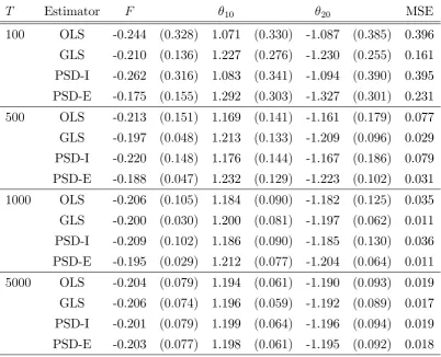
We illustrate the performance of our closed-form estimator using the Monte Carlo design in Sec-tion 7 of Pesendorfer and Schmidt-Dengler (2008); who also provide further comparison with other estimators in the literature.
Setup
Consider a symmetric two-…rm dynamic entry game. In each period t, each …rm i(= 1;2) has two possible choices: be active or not active, ait 2 f0;1g, where 0 corresponds to “not active” and
1 to “active” . Publically observed state variable has four elements, and can be represented by the
6The estimator of Hotz et al. (1994) has an additional source of sampling error since they estimate the discounted
expected payo¤s, E[Vi; i(st+1)jxt; ait], by forward simulation. However, under suitable conditions, the error from
actions made by both …rms in period t 1, so that xt = (a1t 1; a2t 1). The vector of states evolves
over time according to the transition st+1 =at. Firm10s period payo¤s are described as follows:
1; (a1t; a2t; xt) = 1[a1t= 1] [ 1+ 2a2t] +1[a1t= 1; a1t 1 = 0] F +1[a1t = 0; a1t 1 = 1] W;
where ( 1; 2; F; W) denote respectively the monopoly pro…t, duopoly pro…t, entry cost and scrap
value that …rm 1may obtain. Each …rm also receives additive private shocks that are i.i.d. N(0;1). The game is symmetric and …rm’s 2 payo¤s are de…ned analogously.
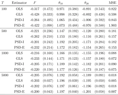
We set ( 10; 20; F0; W0) = (1:2; 1:2; 0:2;0:1). Pesendorfer and Schmidt-Dengler (2008, p.920)
show that there are three distinct equilibria (…ve if we permute the identity of the players as there is one symmetric equilibrium). We generate the data using di¤erent equilibria of the game and provide estimates for ( 10; 20; F0) for each equilibrium. W0 is taken as known, since it is not separately
T Estimator F 10 20 MSE 100 OLS -0.244 (0:328) 1.071 (0:330) -1.087 (0:385) 0.396 GLS -0.210 (0:136) 1.227 (0:276) -1.230 (0:255) 0.161 PSD-I -0.262 (0:316) 1.083 (0:341) -1.094 (0:390) 0.395 PSD-E -0.175 (0:155) 1.292 (0:303) -1.327 (0:301) 0.231
500 OLS -0.213 (0:151) 1.169 (0:141) -1.161 (0:179) 0.077 GLS -0.197 (0:048) 1.213 (0:133) -1.209 (0:096) 0.029 PSD-I -0.220 (0:148) 1.176 (0:144) -1.167 (0:186) 0.079 PSD-E -0.188 (0:047) 1.232 (0:129) -1.223 (0:102) 0.031
1000 OLS -0.206 (0:105) 1.184 (0:090) -1.182 (0:125) 0.035 GLS -0.200 (0:030) 1.200 (0:081) -1.197 (0:062) 0.011 PSD-I -0.209 (0:102) 1.186 (0:090) -1.185 (0:130) 0.036 PSD-E -0.195 (0:029) 1.212 (0:077) -1.204 (0:064) 0.011
[image:22.595.98.501.196.522.2]5000 OLS -0.204 (0:079) 1.194 (0:061) -1.190 (0:093) 0.019 GLS -0.206 (0:074) 1.196 (0:059) -1.192 (0:089) 0.017 PSD-I -0.201 (0:079) 1.199 (0:064) -1.196 (0:094) 0.019 PSD-E -0.203 (0:077) 1.198 (0:061) -1.195 (0:092) 0.018
Table 1: Monte Carlo results (Equilibrium 1). OLS and GLS are our closed-form estimators that are ine¢ cient and e¢ cient respectively. PSD-I and PSD-E are asymptotic least squares
T Estimator F 10 20 MSE 100 OLS -0.317 (0:472) 0.971 (0:380) -0.891 (0:543) 0.822 GLS -0.428 (0:333) 0.998 (0:328) -0.892 (0:438) 0.598 PSD-I -0.264 (0:495) 1.065 (0:434) -1.006 (0:592) 0.843 PSD-E -0.422 (1:098) 1.073 (0:488) -0.976 (0:588) 1.903
500 OLS -0.221 (0:236) 1.147 (0:192) -1.120 (0:280) 0.181 GLS -0.262 (0:210) 1.153 (0:180) -1.116 (0:261) 0.157 PSD-I -0.201 (0:242) 1.192 (0:205) -1.171 (0:284) 0.182 PSD-E -0.232 (0:214) 1.172 (0:182) -1.154 (0:265) 0.153
1000 OLS -0.216 (0:168) 1.166 (0:135) -1.155 (0:196) 0.088 GLS -0.233 (0:144) 1.171 (0:123) -1.157 (0:180) 0.072 PSD-I -0.205 (0:171) 1.189 (0:142) -1.182 (0:201) 0.090 PSD-E -0.220 (0:150) 1.177 (0:126) -1.173 (0:187) 0.075
[image:23.595.98.500.197.522.2]5000 OLS -0.205 (0:076) 1.192 (0:058) -1.189 (0:091) 0.018 GLS -0.203 (0:037) 1.196 (0:039) -1.195 (0:050) 0.005 PSD-I -0.202 (0:076) 1.197 (0:061) -1.196 (0:092) 0.018 PSD-E -0.200 (0:043) 1.197 (0:040) -1.201 (0:058) 0.007
Table 2: Monte Carlo results (Equilibrium 2). OLS and GLS are our closed-form estimators that are ine¢ cient and e¢ cient respectively. PSD-I and PSD-E are asymptotic least squares
T Estimator F 10 20 MSE 100 OLS -0.304 (0:475) 0.997 (0:398) -0.895 (0:558) 0.840 GLS -0.436 (0:356) 1.015 (0:352) -0.88 (0:446) 0.641 PSD-I -0.241 (0:514) 1.102 (0:471) -1.023 (0:624) 0.917 PSD-E -0.397 (0:445) 1.081 (0:381) -0.975 (0:526) 0.722
500 OLS -0.225 (0:244) 1.149 (0:187) -1.118 (0:282) 0.184 GLS -0.26 0 (0:229) 1.159 (0:185) -1.122 (0:278) 0.175 PSD-I -0.201 (0:258) 1.200 (0:222) -1.176 (0:304) 0.208 PSD-E -0.230 (0:239) 1.177 (0:189) -1.157 (0:287) 0.178
1000 OLS -0.214 (0:177) 1.169 (0:134) -1.158 (0:204) 0.093 GLS -0.227 (0:170) 1.179 (0:136) -1.166 (0:206) 0.092 PSD-I -0.202 (0:180) 1.193 (0:147) -1.187 (0:211) 0.099 PSD-E -0.207 (0:186) 1.191 (0:148) -1.188 (0:220) 0.105
[image:24.595.95.502.196.522.2]5000 OLS -0.203 (0:082) 1.194 (0:062) -1.190 (0:093) 0.019 GLS -0.205 (0:076) 1.197 (0:060) -1.192 (0:090) 0.017 PSD-I -0.201 (0:083) 1.200 (0:066) -1.196 (0:095) 0.020 PSD-E -0.201 (0:078) 1.199 (0:061) -1.197 (0:094) 0.018
Table 3: Monte Carlo results (Equilibrium 3). OLS and GLS are our closed-form estimators that are ine¢ cient and e¢ cient respectively. PSD-I and PSD-E are asymptotic least squares
The results are as expected from the theory. At smaller sample sizes the estimators are genuinely di¤erent regardless of the choice of weight matrices. Since the model is fully parametric both e¢ cient estimators generally perform better than the ine¢ cient ones even at T = 100 across all equilibria. With larger sample sizes the ine¢ cient and e¢ cient estimators seem to have similar properties for both methods. Although, in theory, the ine¢ cient estimators need not be asymptotically equivalent as both are weighed by the same identity matrix (see equation (17) in the Appendix).
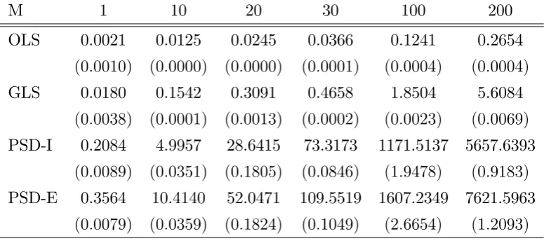
We now abstract away from the statistical properties and consider the numerical aspects. To illustrate the potential for computational advantages of our estimator, we introduce an additive market …xed e¤ect to the per period payo¤ in the game described above. We use the number of markets, denoted by M, to control the complexity of the game.7 For each M, we solve the model once and simulated …ve times using the symmetric equilibrium. We report in Table 4, the average central processing unit (CPU) times in seconds to compute our estimators and ALSEP SD that minimize their respective limiting objective functions (no sampling error, using true choice and transition probabilities); standard errors are in parentheses.8
M 1 10 20 30 100 200
OLS 0.0021 0.0125 0.0245 0.0366 0.1241 0.2654
(0:0010) (0:0000) (0:0000) (0:0001) (0:0004) (0:0004)
GLS 0.0180 0.1542 0.3091 0.4658 1.8504 5.6084
(0:0038) (0:0001) (0:0013) (0:0002) (0:0023) (0:0069)
PSD-I 0.2084 4.9957 28.6415 73.3173 1171.5137 5657.6393
(0:0089) (0:0351) (0:1805) (0:0846) (1:9478) (0:9183)
PSD-E 0.3564 10.4140 52.0471 109.5519 1607.2349 7621.5963
[image:25.595.105.493.351.523.2](0:0079) (0:0359) (0:1824) (0:1049) (2:6654) (1:2093)
Table 4: Computation time. OLS and GLS are our closed-form estimators that are ine¢ cient and e¢ cient respectively. PSD-I and PSD-E are asymptotic least squares estimators of Pesendorfer and
Schmidt-Dengler (2008) that are ine¢ cient (identity weighted) and e¢ cient respectively.
Our estimators are substantially faster to compute, and the distinction grows exponentially with more parameters in the model. The reported CPU times also include the construction of the optimal
7There are other ways to vary the complexity of the game, e.g. by changing the number of potential actions and
states. However, the di¢ culty to solve and estimate such games increases signi…cantly as the games become more complexed. Our design is chosen for its simplicity as it only requires us to solve a simple game multiple times.
8The simulation was performed using MATLAB (R2012a, 64 bit version) on a standard PC running on an Intel
weighting matrices, using numerical derivatives, for GLS and PSD-E. The procedure to compute the optimal weighting matrices are similar for both (asymptotic least squares) estimators, so its contribution in this setting can be approximated by comparing the CPU times of OLS and GLS as M varies. Our results are model speci…c and we precaution against extrapolations as di¤erent designs, as well as algorithms and softwares, will have di¤erent convergence properties for ALSEP SD. Although a claim that closed-form estimation is generally a much simpler task is quite innocuous. We also expect the computation time for ALSEP SD to grow at a faster rate with larger action and/or state spaces for any …xed M. Indeed another, perhaps even more important, numerical property of our closed-form estimators is they are always global minimizers. In contrast, a numerical solution to a general nonlinear optimization routine can be sensitive to the search algorithm, initial values, and as well as the nature of the objective function.9
5
Conclusions and Possible Extensions
We have shown there can be some non-trivial computational gains in de…ning estimators that opti-mize objective functions constructed in terms of expected payo¤s instead of choice probabilities for the estimation of structural dynamic discrete choice problems. The most transparent advantages of our approach follow from an opportunity to utilize familiar linear regression techniques, which arise when the period payo¤ functions are modeled to have fully or partially linear-in-parameter struc-ture. Since the class of estimators we propose is asymptotically equivalent to the unifying class of estimators developed by Pesendorfer and Schmidt-Dengler (2008), there appears to be no theoretical costs associated with our approach to simplify and improve the numerical aspects of the estimation problem. Our estimators also perform well in Monte Carlo exercises in terms of speed and statistical properties.
The computation advantages we describe in this paper accumulates beyond the procedure to obtain a point estimate. For instance, resampling methods that are often used in practice to obtain standard errors (or perhaps to improve …nite sample properties) clearly would bene…t. The type of objective functions we propose also naturally complements other research in the literature that aims to improve the performance and/or scope of two-step methodologies. Two traditional criticisms of two-step estimators are large …nite sample bias (from the …rst stage nonparametric estimation of choice probabilities), and the inability to accommodate unobserved heterogeneity and state variables that are persistent over time. For the former, Aguirregabiria and Mira (2002,2007) propose an
9It is easy to construct a game where the (limiting) objective function de…ned using pseudo-probabilities has multiple
iteration scheme that can improve the …nite sample properties by imposing some structure for the …rst stage estimators; see Kasahara and Shimotsu (2008,2012) for further discussions and some theoretical justi…cations. At each iteration, the structural estimator can update the choice probabilities implied by the pseudo-model that are then used to de…ne a new pseudo-likelihood function. To incorporate our estimator, alternatively one can use the updated probabilities to construct an objective function that de…nes the distance between the (updated) observed and implied expected payo¤s. For the latter, the recent nonparametric identi…cation results of Kasahara and Shimotsu (2009) and Hu and Shum (2012) show any two-step approach can also be readily applied to estimate a more general dynamic model than the one considered in this paper.
Appendix
Proofs of Theorems
Proof of Theorem 1. Under A1 to A3, S( ;W) has a well-separated minimum at 0. Let
( ) = Y X( ) and b( ) = Yb Xb( ). Under A4, it follows that sup 2 k ( )k < 1 and
sup 2 b( ) ( ) =op(1). Then through some tedious algebra, of repeatedly adding nulls and
using properties of the matrix norm:
b
S ;Wc S( ;W) = b( )>Wcb( ) ( )>W ( )
= 2 ( )>W b( ) ( ) +op b( ) ( ) ;
where the smaller order terms are uniform over under A2 - A3. Thereforesup 2 Sb ;Wc S( ;W) =
op(1), and consistency follows from a standard argument (e.g. see Newey and McFadden (1994)).
Proof of Theorem 2. Under our assumptions, b(Wc) satis…es the …rst order condition from di¤erentiating (10) with respect to with probability tending to1, i.e.
0 =
0
@@Xb( )
@ >
=b(Wc)
1 A
>
c
W Yb Xb(b(Wc))
holds with probability tending to 1. SinceY X( 0) = 0, by adding nulls, we have
b
Y Xb(b) = Ub+E1+E2
= Ub rX b(Wc) 0 +op b(Wc) 0 ;
where E1 = X(b(Wc)) X( 0) and E2 = Xb(b(Wc)) Xb( 0) X(b(Wc)) X( 0) , and the
around 0. By adding nulls and using properties of matrix norm, sinceb(Wc) = 0+op(1), we also have @@Xb( )>
=b(Wc)
>
c
W r>XW =op(1) under A2 and A5. Thereforeb(Wc) also satis…es
0 =r>XW Ub rX b(Wc) 0 +op
1
p
N + b(Wc) 0 ;
with probability tending to 1. Then it follows that
p
N b(Wc) 0 = r>XWrX
1
r>XWUb+op(1):
An application of Slutsky’s theorem gives the result.
Proof of Theorem 3. The proof for part (i) is standard (e.g. see Theorem 3.2 of Hansen (1982)). We claim the optimal weighting matrix converges in the limit to 1. LetB =
WrX rX>WrX
1
and C = 1rX rX> 1rX 1, so we have W =B> B and 1 =C> C. Using simple
alge-bra, it can be shown that B> B C> C = (B C)> (B C) 0. For part (ii), it follows from the proof of Theorem 2 that we did not use any speci…c information on Wcbeyond the fact that it has a positive de…nite probability limit.
Representation Lemma
Proof of Lemma R. First we introduce some additional notations that build on the terms de…ned in Section 2.2. Let va
i; i = vi; i(a; x
1); : : : ; v
i; i a; x
J for all a, and v
i; i = v
0
i; i; : : : ; v
K i; i
>
, so that vi; i is a J(K+ 1) vector. Let
a1:::aI
i; i = i; i(a1; : : : ; aI; x
1); : : : ;
i; i a1; : : : ; aI; x
J for all
a1; : : : ; aI, and i; i =
0:::0
i; i ; : : : ;
K:::K i; i
>
, so that i; i is a J(K+ 1)
I
vector. For any k let: Id denote an identity matrix of sized;Hi denote a block-diagonal matrixdiag Hi0; Hi1; : : : ; HiK , where
Hia denotes a J J matrix such that (Hia)jj0 = Pr xt+1 =xj 0
jxt=xj; ait =a ; M= I(K+1)I M
whereM = (IJ L)
1
andLdenotes aJ Jmatrix such that(L)jj0 = Pr xt+1=xj 0
jxt=xj ;R=
2 6 6 4
P0:::0 PK:::K
..
. ...
P0:::0 PK:::K
3 7 7
5be aJ(K+ 1)IbyJ(K+ 1)I matrix, wherePa1:::aI =diag(P(a1; : : : ; aIjx1);
: : : ; P a1; : : : ; aIjxJ ) with P (a1; : : : ; aIjx) = Pr[ 1; 1(sit) = a1; : : : ; I; I(sIt) = aIjxt = x] =
QI
j=1Pj(ajjx), and let Ri =
2 6 6 4
Pi00:::0 PiK:::K0
..
. ...
P0:::0
iK PiKK:::K
3 7 7
5 be a J(K+ 1) by J(K+ 1)I matrix, where
Pa1:::aI
ik = diag(Pik(a1; : : : ; aIjx1); : : : ; Pik a1; : : : ; aIjxJ ) with Pik(a1; : : : ; aIjx) = Pr[ 1; 1(sit) =
Pi(kjx)QIj6=iPj(ajjx). De…ne vi;a i = vi; i(a; x
1) v
i; i(0; x
1); : : : ; v
i; i a; x
J v
i; i 0; x
J for all a > 0; and v = v1
i; i; : : : ; v
K i; i
>
. Let D denote the J KI J(K+ 1)J
matrix that per-forms the transformation Dv = v . Lastly, let vai = vi(a; x1); : : : ; vi a; xJ for alla, and de…ne
vi = v0i; : : : ; vKi >, so that vi =Dvi is aJ(K+ 1) vector. Then (6) immediately follows.
Asymptotic Equivalence of ALSEs
Proof of Proposition E. In the proof of this proposition we shall assume standard regularity conditions hold throughout (i.e. we assume inverse of matrices exist, expected payo¤s and functions are bounded and continuously di¤erentiable etc.). As seen from the proof of Theorem 2, under standard regularity conditions b(Wc) satis…es
b(Wc) = 0+ r>XWrX
1
r>XWUb+op
1
p
N : (15)
Next we introduce ALSEP SD. It shall be useful to bear in mind the illustrative discussion in Section 2.1. We …rst de…ne some additional notations that build on the terms de…ned in Section 2.3. Let P = P>1; : : : ;P>I > and P = P>1;1; : : : ;P>I;
I >
. Similarly, let v = v1>; : : : ; v>I > and
v = v>
1;1; : : : ; v >
I; I >
. Then, by Hotz and Miller’s inversion there exists an invertible and continuously di¤erentiable map such thatP= ( v) and P = ( v ). In particular
P = 1( v1)>; : : : ; I( vI)>
>
; and
P = 1( v1; 1) >; : : : ;
I( vI; I) > >;
where i is the inverse of i, which is de…ned in the text. Therefore, in terms of Y and X ( ),
v v =Y X ( ).
Thus P and P are also deterministic functions of the preliminary estimators (that we denoted by
0). We denote the estimators of P and P by Pe and Pb respectively, and these estimators are
constructed based on the same bthat de…neXb and Yb. Note that, althoughP=P 0,Pe and Pb 0 are generally di¤erent. An ALSEP SD, denoted bybP SD(Vb), is de…ned as the minimizer of
min
2 Pe Pb >
b
V Pe Pb ;
for some Vb that converges in probability to positive de…nite matrix V (cf. equation (21) on page 915 in Pesendorfer and Schmidt-Dengler (2008)). Under appropriate regularity conditions, it is straightforward to show, analogous to our Theorem 2, that
p
N bP SD(Vb) 0
d
For a …rst order asymptotic equivalence, it su¢ ces to only consider the local asymptotic properties of ALSEP SD around 0. Let rP denote @@P> =
0. An ALSEP SD satis…es
0 = r>PV Pe P Pbb
P SD(V) P 0 +op
1
p
N :
As the problem is smooth, it can be shown generally that the condition above simpli…es further to
0 = r>PV Pe P Pb 0 P 0 +Pb
P SD(V) P 0 +op
1
p
N :
So that we have
bP SD(V) = 0+ r>PVrP 1
r>PV Pe P (Pb 0 P 0) +op
1
p
N :
By chain rulerP equalsr rX, wherer denotes the Jacobian of evaluated at v, and @@ v> =
0
equals rX. Thus, we can write
bP SD(V) = 0+ r>Xr>Vr rX
1
r>Xr>V Pe P (Pb 0 P 0) +op
1
p
N
= 0+ r>Xr>Vr rX
1
r>Xr>Vr Ub+op
1
p
N ;
where the last equality follows from linearizing Pe P (Pb 0 P 0) in terms of Yb Xb( 0). By
de…ning WV =r>Vr , we have
bP SD(V) = 0 + r>XWVrX
1
r>XWVUb+op
1
p
N : (16)
Therefore, by comparing (15) and (16), bP SD(V) has the same asymptotic distribution as b(WV).
In particular, let V denote the e¢ cient weighting matrix for ALSEP SD so that V V for any positive de…nite matrix V. Therefore the e¢ cient ALSEP SD, denoted by bP SD, has the same asymptotic distribution asb(WV )with WV =r>V r . Then it must hold, by Theorem 3(i), that
1 V since 1 is the lower variance bound. To complete the proof, an identical argument
can be made in the reverse direction. It is easy to show that anyb(W)that satis…es (15) also has the same asymptotic distribution as bP SD(VW), where VW =r> 1Wr 1 (cf. WV), andr 1 denotes
the Jacobian of 1 evaluated at P (that equals (
r ) 1 by the inverse function theorem). We omit further details to avoid repetition. Thus, it follows that V 1, hence we can also conclude
that V = 1.
In summary:
p
N b(W) 0 = p
N bP SD(VW) 0 +op
1
p
N with VW =r
>
1Wr 1, (17)
p
N bP SD(V) 0 = p
N b(WV) 0 +op
1
p
N with WV =r
>
and (V;W) can be replaced by any consistent estimators (Vb;Wc). Therefore our estimator and ALSEP SD can always be constructed to have the same asymptotic distribution and achieve the same lower variance bound.
References
[1] Ackerberg, D., L. Benkard, S. Berry, and A. Pakes (2005), “Econometric Tools for Analyzing Market Outcome,”Handbook of Econometrics, vol. 6, eds. J. Heckman and E. Leamer. North-Holland.
[2] Aguirregabiria, V., and P. Mira (2002): “Swapping Nested Fixed Point Algorithm: a Class of Estimators for Discrete Markov Decision Models,”Econometrica, 70, 1519-1543.
[3] Aguirregabiria, V. and P. Mira (2007): “Sequential Estimation of Dynamic Discrete Games,”
Econometrica,75, 1-53.
[4] Aguirregabiria, V., and P. Mira (2010): “Dynamic Discrete Choice Structural Models: A Sur-vey,”Journal of Econometrics, 156, 38-67
[5] Aguirregabiria, V. and J. Suzuki (2013): “Identi…cation and Counterfactuals in Dynamic Models of Market Entry and Exit,”Working Paper, University of Toronto.
[6] Amemiya, T. (1985): Advanced Econometrics, Harvard University Press.
[7] Bajari, P. and H. Hong (2006): “Semiparametric Estimation of a Dynamic Game of Incomplete Information,”NBER Technical Working Paper 320.
[8] Bajari, P., C.L. Benkard, and J. Levin (2007): “Estimating Dynamic Models of Imperfect Competition,”Econometrica, 75, 1331-1370.
[9] Bajari, P., V. Chernozhukov, H. Hong and D. Nekipelov (2009): “Identi…cation and E¢ cient Estimation of a Dynamic Discrete Game,”Working paper, University of Minnesota.
[10] Chamberlain, G. (1982): “Multivariate Regression Models for Panel Data,”Journal of Econo-metrics, 18, 5-46.
[11] Collard-Wexler, A. (2013): “Demand Fluctuations and Plant Turnover in the Ready-Mix Con-crete Industry,”forthcoming in Econometrica.