Evaluating treatment effectiveness under model misspecification: A comparison of targeted maximum likelihood estimation with bias-corrected matching

(1)

City, University of London Institutional Repository

Citation

:

Kreif, N., Gruber, S., Radice, R. ORCID: 0000-0002-6316-3961, Grieve, R. and

Sekhon, J. S. (2016). Evaluating treatment effectiveness under model misspecification: A

comparison of targeted maximum likelihood estimation with bias-corrected matching.

Statistical Methods in Medical Research, 25(5), pp. 2315-2336. doi:

10.1177/0962280214521341

This is the accepted version of the paper.

This version of the publication may differ from the final published

version.

Permanent repository link:

http://openaccess.city.ac.uk/20769/

Link to published version

:

http://dx.doi.org/10.1177/0962280214521341

Copyright and reuse:

City Research Online aims to make research

outputs of City, University of London available to a wider audience.

Copyright and Moral Rights remain with the author(s) and/or copyright

holders. URLs from City Research Online may be freely distributed and

linked to.

(2)

Evaluating treatment

effectiveness under model

misspecification: A comparison

of targeted maximum likelihood

estimation with bias-corrected

matching

Noe´mi Kreif,

1

Susan Gruber,

2

Rosalba Radice,

3

Richard Grieve

1

and Jasjeet S. Sekhon

3

Abstract

Statistical approaches for estimating treatment effectiveness commonly model the endpoint, or the propensity score, using parametric regressions such as generalised linear models. Misspecification of these models can lead to biased parameter estimates. We compare two approaches that combine the propensity score and the endpoint regression, and can make weaker modelling assumptions, by using machine learning approaches to estimate the regression function and the propensity score. Targeted maximum likelihood estimation is a double-robust method designed to reduce bias in the estimate of the parameter of interest. Bias-corrected matching reduces bias due to covariate imbalance between matched pairs by using regression predictions. We illustrate the methods in an evaluation of different types of hip prosthesis on the health-related quality of life of patients with osteoarthritis. We undertake a simulation study, grounded in the case study, to compare the relative bias, efficiency and confidence interval coverage of the methods. We consider data generating processes with non-linear functional form relationships, normal and non-normal endpoints. We find that across the circumstances considered, bias-corrected matching generally reported less bias, but higher variance than targeted maximum likelihood estimation. When either targeted maximum likelihood estimation or bias-corrected matching incorporated machine learning, bias was much reduced, compared to using misspecified parametric models.

Keywords

targeted maximum likelihood estimation, bias-corrected matching, treatment effectiveness, machine learning, double robustness, model misspecification

1

Department of Health Services Research and Policy, London School of Hygiene and Tropical Medicine, London, UK

2

Department of Epidemiology, Harvard School of Public Health, Boston, MA, USA

3

Birkbeck, University of London, London, UK

4

Travers Department of Political Science, UC Berkeley, Berkeley, CA, USA

Corresponding author:

Noe´mi Kreif, Department of Health Services Research and Policy, London School of Hygiene and Tropical Medicine, 15–17 Tavistock Place, London WC1H 9SH, UK.

Email: [email protected]

Statistical Methods in Medical Research 0(0) 1–22

!The Author(s) 2014 Reprints and permissions:

(3)

1 Introduction

Health policy makers require unbiased, precise estimates of the effectiveness and cost-effectiveness of health interventions.1–3When observational studies are used to estimate average treatment effects (ATEs), it is vital to address potential bias due to confounding. Most studies use methods that assume there is no unmeasured confounding.4 Under this assumption unbiased estimates can be obtained after controlling for observed characteristics, for example with parametric regression, propensity score (PS) or double-robust (DR) methods, provided either the PS or the endpoint regression model is correctly specified.

In studies that rely on regression methods alone, the estimated ATEs can be highly sensitive to the choice of model specification.5 When evaluating health care interventions, correctly specifying a regression model can be challenging. For example, health-related quality of life (HRQoL) data are often semi-continuous, with non-linear covariate–endpoint relationships.6Instead, PS approaches may be preferred such as matching or inverse probability of treatment weighting (IPTW), but these rely on the correct specification of the PS. Most medical applications use a PS estimated with logistic regression models that only include main effects, which raises the concern of model misspecification.7,8

DR methods9,10 are consistent if either the endpoint regression or the PS is correctly specified. However, in practice both the regression function and the PS may be misspecified, and also, poor overlap can lead to the estimated PSs close to 0 and 1.11 Here, DR methods such as weighted regression may not protect from bias.12,13 A recently proposed DR method, targeted maximum likelihood estimation (TMLE),14,15 can be less biased and more efficient than conventional DR methods when there is poor overlap16–18 by respecting known bounds on the endpoint. Another approach which can exploit information from the PS and the endpoint regression is bias-corrected matching (BCM).19,20This method aims to reduce residual bias by adjusting the matching estimator with regression predictions of the endpoint. BCM is relatively robust under misspecification, for example, unless the functional form relationship between the covariates and the endpoint is highly non-linear; adjustment using a linear regression for the endpoint can reduce most of the residual bias from imbalance in the matched data.20–23However, an outstanding concern with TMLE and BCM that use fixed, parametric models is that there may be residual bias due to functional form misspecification of both the PS and endpoint regressions.

In order to minimise bias due to functional form misspecification, both methods can exploit machine learning techniques. Unlike fixed, parametric models, where the functional form is chosen by the analyst, these methods use an algorithm to find the best fitting model. Machine learning estimation approaches for estimating the PS8,24,25 and the endpoint regression function26 have been shown to reduce bias due to model misspecification. However, few studies have investigated machine learning for DR approaches.16,27 No previous study has considered machine learning for BCM.

This paper aims to compare TMLE and BCM and to combine both methods with machine learning for estimating the PS and the endpoint regression function. The methods are contrasted for estimating the ATE of a binary treatment, with a focus on dual functional form misspeciﬁcation of the PS and the endpoint regression. We also compare TMLE and BCM to other commonly applied DR,12PS matching28,29 and regression6approaches.

(4)

regression function. The simulation study was grounded in the case study and compared the relative performance of the methods for a range of data generating processes (DGPs). We compare the relative performance of the methods according to bias, root mean squared error (RMSE) and coverage rates of nominal 95% conﬁdence intervals (CIs).

In the next section, we outline the statistical methods under comparison. Section 3 presents the motivating example. Section 4 reports the design and results of the simulation study. The last section discusses the ﬁndings and suggests areas for further research.

2 Statistical methods

The parameter of interest is the ATE of a binary treatmentA, deﬁned as

¼E½Yð Þ 1 Yð Þ0

whereYð1Þis the potential outcome under treatment, i.e. the endpoint that would be observed under the treatment state, and Yð Þ0 is the potential outcome under the control state. The vector of confounding factors, that is all factors that inﬂuence the potential outcomes and treatment assignment, is deﬁned as W. Under the assumption of no unmeasured confounders,32all elements

of W are observed, and the mean of the conditional distribution of the potential outcomes

corresponds with the mean of the conditional distribution of the observed endpointY

E Y½ ð1ÞjW ¼E Y½ jA¼1,W and E Y½ ð0ÞjW ¼E Y½ jA¼0,W

Under the additional assumptions of consistency and positivity, the ATE can be identiﬁed as

¼E E Y ½ jA¼1,W E Y½ jA¼0,WjW

where the (potentially heterogeneous) individual level treatment effects are marginalised over the distribution of WThe consistency assumption states that an individual’s potential outcome under the observed treatment is exactly the observed endpoint.33 The positivity assumption requires that there are both treated and control individuals at each combination of the values of observed confounders in the population,11formally, 05g A,ð WÞ51, for any stratum defined byW, where g A,ð WÞ ¼PðAjWÞis the model for the treatment assignment. In finite samples, positivity violations often arise; in particular covariate strata there might be few or no individuals from either treatment group,11and so the estimatedg A,^ð WÞcan be close to 0 or 1. The econometric literature on matching methods refers to positivity violations as ‘poor overlap’,34and we use this terminology throughout the paper.

2.1 Regression estimators

We consider a general regression estimator, the G-computation estimator,35which uses estimates of

the expected potential outcomes, conditional on observed characteristics, deﬁned as

Q A,ð WÞ ¼E Y½ jA,W. The estimator for the ATE is given by

^reg_¼ 1

N

XN i¼1

^

Qð1,WiÞ Q^ð0,WiÞ

n o

(5)

where Q^ð1,WÞ and Q^ð0,WÞ are the estimated potential outcomes for each individual under treatment and control states, respectively, andNis the number of subjects in the sample.

^

Qð0,WÞ and Q^ð1,WÞ can be obtained by fitting a regression model that includes the observed covariates and a treatment variable, for example ordinary least squares (OLS) regression or a generalised linear model (GLM). A more flexible method is to fit separate models for the treatment and control samples.36 When there is poor overlap, regression estimators extrapolate, which can lead to large biases if the regression model is misspecified.5,37

2.1.1 Machine learning estimation of the regression function

In general, machine learning covers a wide range of classification and prediction algorithms.8,26 Unlike approaches that assume a fixed statistical model, for example a GLM with a log link, machine learning aims to extract the relationship between the endpoint and covariates through a learning algorithm.24 Machine learning approaches for estimating the endpoint regression can reduce bias which results from model misspecification.26 Here we consider the ‘super learning’ algorithm,38 which uses cross-validation to select a weighted combination of estimates given by different prediction procedures.39 The range of prediction algorithms is pre-selected by the user, potentially including parametric and non-parametric regression models. Asymptotically, the super learner algorithm performs as well as the best possible combination of the candidate estimators.40

2.2 PS methods

The PS, deﬁned as the conditional probability of treatment assignment given W, gð1jWÞ ¼

PrðA¼1jWÞ, can create balance between the distributions of observed confounders of the

treatment and control samples.41 The PS matching estimator imputes the missing potential

outcomes, Yð Þ0 or Yð Þ1, for each individual, using the observed endpoints of the closest M individuals (the matches), where closeness is measured by the estimated PS,g^ðA¼1,WÞ

^

Yð0,WiÞ ¼

Yi ifAi¼0

1 M

X

jMðiÞ

Yj ifAi¼1

8 > < > : ^

Yð1,WiÞ ¼

1 M

X

jMðiÞ

Yj ifAi¼0

Yi ifAi¼1

8 > < > :

and whereMðiÞ is the set ofMindividuals from the opposite treatment group, matched to uniti.

The estimator for the ATE is the mean of the estimated individual-level treatment eﬀects

^match_¼ 1

N

XN i¼1

^

Yð1,WiÞ Y^ð0,WiÞ

n o

IPTW reweights the treated and control samples using inverse weights Ai

^

gð1jWiÞ for the treated and

1Ai

1g^ð1jWiÞ for the control observations. The normalised IPTW estimator

12,42

is deﬁned as

^IPTW_¼

PN

i¼1Ai_g_^ð1YjWi iÞ

PN i¼1g^ð1AjWi iÞ

PN

i¼1ð1AiÞ₁g^Yð1ijWiÞ

PN

(6)

Matching estimators are consistent ifg^ðÞis correctly specified,43but can have finite sample bias, and are less precise than a correctly specified regression estimator.19,44 With a correctly specifiedg^ðÞ, IPTW can also provide consistent and efficient estimates.45 However, poor overlap can result in unstable inverse probability of treatment (IPT) weights, and biased or inefficient estimates of the ATEs, even when g^ðÞ is correctly specified.12,21,24,46 In these settings, recommended approaches include stabilising IPT weights,47truncating IPT weights at fixed levels48or percentiles ofg^ðÞ47as well as estimating ATEs for a subsample with good overlap.49

2.2.1 Machine learning estimation of the PS

Instead of estimating the PS with a fixed parametric model, flexible approaches have been proposed to help correctly specifygð Þ:. These include the series regression estimator,45and methods from the machine learning literature, including decision trees, neural networks, linear classifiers and boosting.8,25,50 This paper considers boosted classification and regression trees (CART), as it has been shown to reduce bias in the estimated ATE compared to a misspecified logistic regression, and

other machine learning methods such as pruned CARTs.24 When performing boosted CARTs,

regression trees are ﬁt on random subsets of the data, and in each iteration, the data points that were incorrectly classiﬁed with the previous trees receive greater priority. According to general

recommendations,51 the algorithm can be set to select the ﬁnal PS model that maximises

covariate balance.24,50

2.3 DR methods

DR methods9,52combine models forQð Þ: andgð Þ:, with most estimators usingg^ð Þ: to construct IPT weights.53 The distinctive property of DR estimators is that they are consistent if either (but not necessarily both)g() orQ() is correctly specified.9If both components are correct, the DR estimator can be a semi-parametric efficient estimator.10,15A commonly used DR method is the weighted least squares (WLS) regression,12,13which weights the covariates in a linear regression, using IPT weights. In realistic settings such as when there is poor overlap and dual misspecification, weighted regression can report biased and inefficient estimates of ATEs.12,13,16,54 An ongoing debate discusses the relative merits of different DR estimators in these circumstances.10,16,55 One recommendation is to use machine learning methods to estimate g().27 A further suggestion is that DR estimators should have a ‘boundedness property’: they should respect the known bounds of the endpoint – for example that an HRQoL endpoint ranges from the value for the worst imaginable health state (0.59) to that for full health, 156 – so that the estimated parameter will always fall into the parameter space.10,57This property can reduce bias and increase precision when the PS is used as weights, where large weights can lead to estimated values of the endpoint falling outside of a plausible range.18 Below we discuss a DR estimator, TMLE, that can have this boundedness property57and is therefore appealing when overlap is poor.18,58

2.3.1 TMLE

(7)

Performing TMLE involves two stages,61which, for estimating the ATE, are

(1) Obtain an initial estimate of the conditional mean ofYgivenAandW, by using regression to predict the potential outcomesQ(1,W) andQ(0,W).

(2) Fluctuate this initial estimate,Q^0ðA,WÞ, by exploiting information in the treatment assignment mechanism.

Here, the ﬂuctuation corresponds to extending the parametric model for Q A,ð WÞ with an additional covariateh, which is a function of the PS

h A,ð WÞ ¼ A

gðA¼1jWÞ

1A

1gðA¼1jWÞ

In the extended parametric model, Q1_ð_A,_W_{Þ ¼}_Q0_ð_A,_W_{Þ þ}_"_h_ð_A,_W_Þ_, _" _{is ﬁtted by maximum}

likelihood. hðA,WÞ is defined so that the solution of the score equation of this model implicitly also solves the efficient influence curve estimating equation for the ATE parameter. In practice, this translates to regressing the observed endpoint onhand an initial estimatecQ0_ð_A,_W_Þ_{as offset. This}

regression can be interpreted as explaining any residual variability after the initial estimate, using information from the treatment assignment mechanism.

To ensure the boundedness of the TMLE, for continuous endpoints it is recommended that known bounds of the endpoint are exploited by rescalingYto between 0 and 1.18,58 The rescaled

endpoint is deﬁned as Y_¼Ya

ba, where a and b are known limits of Y. Using Y*,

Q_ð_A,_W_{Þ ¼}Q Að ,WÞa

ba can be deﬁned. The ﬂuctuation can then be performed on the logistic scale

logitQc1_ð_A,_W_Þ_¼_logit_c_Q0_ð_A,_W_Þ_þ_"_^_b_h_ð_A,_W_Þ

Here,"^can be estimated by logistic regression, where the mean of the outcome, bounded between 0 and 1, is modelled with a quasi-binomial distribution, by regressing Y _on _h_^_ð_A,_W_Þ _{with oﬀset} logitQc0_ð_A,_W_Þ_: _Q_^1_ð_A,_W_Þ _{can be obtained by back-transforming} _c_Q1_ð_A,_W_Þ _{to the original}

scale. The resulting targeted estimates of the potential outcomes Q^1_ð_0,_W_Þ _and _Q^1_ð_1,_W_Þ _are

applied in the G-computation formula in order to obtain the TMLE

^TMLE _¼1

N

XN i¼1

^

Q1ð1,WiÞ Q^

1

0,Wi

ð Þ

TMLE can use predictions from any ﬁxed parametric model for the initialQðÞ(e.g. OLS or GLM) andgðÞ(e.g. logistic regression). However, with machine learning methods, TMLE has been shown to reduce bias when the models for the assignment mechanism and the endpoint are misspeciﬁed.16 As in the previous sections, we consider super learning for the initial QðÞ and boosted CARTs forgðÞ.

2.3.2 BCM

(8)

of the endpoint on covariates, stratiﬁed by treatment assignment. The bias-corrected predictions of the potential outcomes are obtained as follows

^

Yð0,WiÞ ¼

Yi ifAi¼0

1 M

X

jMðiÞ

YjþQ^ð0,WiÞ Q^ 0,Wj

ifAi¼1

8 > < > :

^

Yð1,WiÞ ¼

1 M

X

jMðiÞ

YjþQ^ð1,WiÞ Q^ 1,Wj

ifAi¼0

Yi ifAi¼1

8 > < > :

For example, for an individual i who receives control, the imputed potential outcome under the treatment state is the average observed outcome of theMclosest matches from the treatment group (indexed byj), adjusted with the diﬀerence between the predicted outcomes when covariate values are set to those of its own values, Q^ð1,WiÞ and the covariate values of the match, Q^ 1,Wj

. The corresponding estimator is the mean diﬀerence of these bias-corrected predicted potential outcomes

^BCM_¼ 1

N

XN i¼1

^

Yð1,WiÞ Y^ð0,WiÞ

BCM is consistent ifQð0,WÞandQð1,WÞare consistently estimated20 or when the PS is correctly specified. Matching can decrease the sensitivity of estimates to the misspecification of the endpoint regression model5 and, for moderately non-linear response surfaces, adjustment even with a misspecified OLS model can reduce bias.19–22 Because an OLS regression, even including non-linear terms, might not capture highly non-non-linear response surfaces, we consider super learning for predicting the potential outcomes, as well as fixed parametric models. We implement 1-to-1 matching because increasing the number of matches would result in larger distances between matched treated and control units, and therefore increase bias.29,51,63 We match on the linear predictor of PS with replacement, allowing for ties. We estimate the PS using logistic regression and also using boosted CARTs.

3 Motivating case study

3.1 Overview

We consider the methods in a case study that evaluates the effect of alternative hip prosthesis types on the HRQoL of patients with osteoarthritis using an observational database on patients with THR. THR is one of the most common surgical procedures in the UK, with over 50,000 hip procedures performed in the National Health Service (NHS) in England and Wales in 2011;64 health care decision makers have a considerable interest in evaluating the effectiveness of different prosthesis types in routine care.64 A large-scale survey that collects PROMs on all patients who undergo elective surgery in the NHS provides a key data source for this evaluation. The resulting observational dataset includes pre- and post-operative HRQoL for patients with THR procedures.30,31

(9)

population to give utility index scores on a scale ranging from 1 (perfect health), through 0 (death) to the worst possible health state,0.59.56This results in a bounded, semi-continuous distribution of the endpoint that exhibits a point mass at 1, posing a challenge for the speciﬁcation of the regression model.6

A previous analysis of this dataset66 reported the relative eﬀectiveness of common prosthesis types, such as cemented, cementless and ‘hybrid’ prostheses. The analysis used multivariate matching and linear regression to adjust for confounding and found a small but statistically signiﬁcant advantage of hybrid compared to cementless prostheses.

For this motivating example, we estimate the ATE on EQ-5D-3L, 6 months after THR in males patients, aged 65–74 (n¼3583) who received hybrid versus cementless hip prostheses. We illustrate the use of TMLE and BCM with ﬁxed parametric models and then machine learning estimation techniques, and compared to regression, matching, IPTW and WLS.

3.2 Statistical methods in the case study

Potential confounders include patient characteristics such as age, sex, body mass index, pre-operative health status (‘Oxford Hip score’ and HRQoL), comorbidities, disability, index of multiple deprivation and characteristics related to the intervention, such as surgeon experience (senior surgeon or not) and hospital type (NHS, private sector hospital or treatment centre). Of the 3583 patients included in the analysis, 70% had a missing value on at least one variable, with 46% having missing values for more than one covariate. Thirty-two per cent were missing data on post-operative HRQoL and 39% on BMI. Other covariates were complete for over 90% of the sample. Multiple imputation using chained equations was applied to impute missing covariate and endpoint values.66Following recommendations,67ﬁve multiply imputed datasets were created, and the analysis described below was performed on each dataset. Point estimates and variances were combined using Rubin’s formulae.68Fixed parametric approaches for estimatingQðÞincluded OLS regression and a two-part model which can account for the point mass in the observed distribution of the endpoint.6,69,70Here the binary partPðY51Þwas modelled with logistic regression, while a

gamma regression was used for modelling the continuous part ðY0_¼₁_Y _when _Y₅₁_Þ_.

Continuous covariate effects were modelled flexibly using smooth functions which are approximated by a linear combination of known spline basis functions and regression parameters. Such parameters were estimated by fitting generalised additive models using the R package ‘splines’, with default degrees of freedom of 4.71

For machine learning estimation of QðÞ, we used the R package ‘Super Learner’,72 where the user-deﬁned library included the following prediction algorithms: ‘glm’ (main terms linear regression), ‘glm.interaction’ (glm with covariate interactions) and a package that implements multivariate adaptive polynomial spline regression methods, ‘polymars’.73 Machine learning estimation ofgðÞrelied on boosted (logistic) CARTs, using the R package ‘twang’,74 with tuning parameters recommended by the developers.24,50 This implementation aimed to minimise mean covariate imbalance measured using Kolmogorov–Smirnov tests, reweighted by the estimated IPT weights.

We applied WLS with IPT weights obtained from the logistic model and also from the boosted

CARTs. TMLE used the known minimum and maximum values of the endpoint as bounds,0.59

(10)

the super learning regression estimator, standard errors were estimated with the non-parametric bootstrap.75

3.3 Case study results

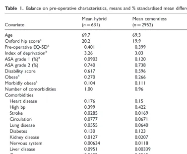
Table 1 presents balance on the main pre-operative characteristics of patients who underwent hybrid versus cementless THR, reported as absolute standardised mean diﬀerences. Patients with hybrid hip replacement were slightly older, had more comorbidities and were less likely to have been treated by a consultant or in a treatment centre.

[image:10.592.86.464.262.573.2]

There was good overlap between the densities of the estimated PSs for the hybrid and cementless groups, whengðÞwas obtained by logistic regression (Figure 1). The plots obtained using boosted CART for estimating the PS were similar.

Table 1. Balance on pre-operative characteristics, means and % standardised mean differences.

Covariate

Mean hybrid (n¼631)

Mean cementless

(n¼2952) SMD (%)

Age 69.7 69.3 15.98

Oxford hip scorea 20.2 19.9 2.83

Pre-operative EQ-5Da 0.401 0.399 0.63

Index of deprivationa _3.26 _3.03 _15.92

ASA grade 1 (%)a 0.0903 0.120 9.55

ASA grade 2 (%) 0.740 0.738 0.52

Disability score 0.617 0.596 4.19

Obesea 0.270 0.266 0.69

Morbidly obesea 0.104 0.111 4.30

Number of comorbidities 1.00 0.96 4.14

Comorbidities

Heart disease 0.176 0.15 7.86

High bp 0.399 0.422 4.55

Stroke 0.0285 0.0169 7.78

Circulation 0.0777 0.0671 4.08

Lung disease 0.0555 0.0640 3.61

Diabetes 0.130 0.123 2.20

Kidney disease 0.0127 0.0207 6.24

Nervous system 0.00634 0.0118 5.20

Liver disease 0.0951 0.00339 7.65

Cancer 0.0602 0.0515 3.80

Depression 0.0491 0.0373 5.84

Consultant 0.803 0.869 17.64

Treatment centre 0.0491 0.122 26.16

Note: SMD: standardised mean difference. SMD was calculated asd¼100jxh_{ffiffiffiffiffiffiffi}xcj s2

hþs

2

c

2

q , where xhand xcare the means for

the hybrid and cementless group, while the denominator includes the pooled standard deviation of the two groups, for a given covariate. Variables are dichotomous, with the exception of age, Oxford hip score, pre-operative EQ-5D-3L score, index of deprivation and number of comorbidities.

(11)

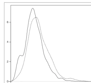
Figure 2 shows the point estimates and 95% CIs after combining the estimates obtained for the imputed datasets. All methods reported a small positive advantage in mean EQ-5D-3L scores for hybrid versus cementless prostheses, but with CIs that included zero.

4 Simulation study

4.1 Overview

The simulation study compares the performance of BCM and TMLE, in estimating the ATE of a binary treatment on an endpoint with a non-linear response surface. As in the case study, we compared these methods to regression, PS matching, IPTW and WLS, and for each method, we

considered ﬁxed parametric models and machine learning estimation for QðÞ and gðÞ.

Motivated by the case study and previous simulation studies,6,16,26 we considered DGPs with non-linear response surfaces; normal, gamma-distributed and semi-continuous endpoints; good and poor overlap and with moderate and strong association between confounders and the endpoints. These DGPs (Table 2) were selected to highlight the diﬀerences between the

0.1 0.2 0.3 0.4 0.5 0.6

[image:11.592.114.408.67.336.2]

0 2 4 6

Figure 1. Densities of the estimated PS using logistic regression, hybrid versus cementless THR. Hybrid (dashed

(12)

performances of the methods under realistic circumstances, by investigating the following hypotheses:

(1) Reweighting methods are anticipated to outperform BCM when overlap is good.21 In such scenarios, TMLE is expected to outperform BCM in terms of bias and eﬃciency.

–0.02 –0.01 0.00 0.01 0.02 0.03 0.04

BCM (SL + boosted CART) BCM (2pt + logistic) BCM (OLS + logistic) TMLE (SL + boosted CART) TMLE (2pt + logistic) TMLE (OLS + logistic) WLS (boosted CART) WLS (logistic) IPTW boosted CART

IPTW logistic PS matching (logistic) Regression (SL) Regression (2 part model) Regression (OLS) Unadjusted

[image:12.592.113.437.69.378.2]

Point estimates and 95% CIs

Figure 2. Point estimates and 95% CIs of ATE in terms of EQ-5D-3L score, hybrid versus cementless THR, across

statistical methods. SL: super learner.

Table 2. Summary of DGPs used in the simulation study.

Overlap

Confounder–endpoint

association Endpoint distribution

DGP 1 Good Moderate Normal

DGP 2 Good Strong Normal

DGP 3 Poor Strong Normal

DGP 4 Poor Strong Gamma

[image:12.592.98.451.441.534.2]

(13)

(2) When overlap is poor, BCM is expected to outperform TMLE, because matching can be less sensitive than weighting to extreme PS values and to the misspeciﬁcation of gðÞ.21,24,43

(3) Using appropriate machine learning methods is anticipated to reduce bias compared to using misspeciﬁed parametric models forQðÞandgðÞ,16,26 across all methods considered.

We assumed a PS mechanism that generated good overlap of the densities of the true PS (DGP 1 and 2) and one that generated poor overlap (DGP 3–5). We considered moderate (DGP 1) and strong (DGP 2–5) association between the confounders and the endpoints. DGPs 1–3 considered a normal endpoint with an identity link function between the linear predictor and the endpoint, DGP 4 considered an endpoint which followed a gamma distribution with a log link, while DGP 5 considered a semi-continuous distribution, with a mixture of a beta-distributed random variable and values of 1.

For each DGP, five scenarios were considered: (a) when fixed parametric models were used for both the PS and the endpoint regression, and these were correctly specified, (b and c) when one of the two was misspecified and (d) when the correct specification for both models was unknown. Scenario (d) had two sub-scenarios, differentiated by the implementation of the methods: in scenario (d1), we considered misspecified, fixed parametric models, while for scenario (d2) we considered machine learning estimates of QðÞ and gðÞ. Here, similarly to (d1), the correct parametric models were unknown for the investigator and were not included among the candidate prediction algorithms. For DGP 1, we report results from each of the five scenarios, while for DGPs 2–5, we only report the results for scenarios (d1) and (d2), as these were a priori judged the most realistic. The results for the remaining scenarios are available upon request.

Bias, variance, RMSE and the coverage rate for nominal 95% CIs of the estimated ATEs were obtained. Relative bias was calculated as the percentage of the absolute bias of the true parameter value, where absolute bias is the diﬀerence between the true parameter value and the mean of the estimated parameter. The RMSE was taken as the square root of the mean squared diﬀerences between the true and estimated parameter values.

4.2 DGPs

For each DGP, we generated 1000 datasets of n¼1000, with binary (W1 to W5) and

standard normally distributed covariates ðW6 to W8Þ. This mix of binary and continuous

covariates reflects the case study. The correlation coefficients between the covariates were set between 0.075 and 0.6. All covariates were true confounders, i.e. they influenced both the treatment assignment and the endpoint. Treatment was assigned according to a true PS

that, like previous simulation studies, included main terms, higher order terms and

interactions.26,43

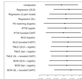
For DGP 1, the PS model resulted in a good overlap of the true PS (see Figure 3)

logit PSð Þ ¼ 1þk1ð0:3W10:1W20:2W3þ0:4W4þ0:7W5

þ0:2W6þ0:2W70:25W8þ0:8W260:3W 2 7

0:3W2₈0:05W1W20:05W1W3Þ

(14)

The treatment variableAwas drawn from a Bernoulli distribution, using the PS as the parameter of success probability. The endpoint was drawn from a normal distribution with mean

norm¼15þ0:4Aþk2ð1W10:1W2þ0:1W30:1W4þ0:1W5

0:1W6þ0:1W7þ0:1W80:2W260:1W270:1W28

þ0:2W3₆þ0:1W3₇þ0:1W3₈0:1W1W2þ0:5W1W7Þ

standard deviation of 1 andk2¼1.

In DGP 2, setting k2 to 4 increased the strength of the confounder–endpoint association. In

DGP 3, changingk1 to 1 created a poor overlap of the true PS distributions (see Figure 3).

In DGP 4, the endpoint was drawn from a gamma distribution, with a log link, shape parameter of 100 and a scale parameter ofgam

100, where the linear predictor was

logðgamÞ ¼3þ0:2A0:2W1þ0:2W20:2W3þ0:5W41W5þ0:5W60:5W7þ0:2W8

[image:14.592.88.470.62.378.2]

0:2W2₆0:01W2₇0:01W2₈0:01W3₆0:01W3₇0:01W3₈0:01W1W20:4W6W7

Figure 3. Densities of the true PS in the simulations for a typical sample (n¼10,000). Treated (dashed line) versus

(15)

In DGP 5, motivated by the case study and previous simulation studies,6the endpoint was generated as a mixture of a beta distributed continuous variableY0and 1, using a Bernoulli distribution with parameterpto select between values from the two distributions

Yð1pÞ 1þpð1Y0Þ

where

logit pð Þ ¼41A0:2W1þ0:5W20:5W31W40:3W5

þ0:2W6þ0:5W70:5W8

Y0_Beta

betaphi,betað1phiÞ

ð Þ,

logitðbetaÞ ¼ 10:2A0:5W10:5W20:5W3þ0:5W40:5W50:5W6

0:5W70:5W80:2W260:2W 2

70:2W 2

80:2W 3

60:2W 3

70:2W 3 8

0:2W1W20:2W6W7Þ

The resulting semi-continuous distribution with a point mass at 1 reflects the observed endpoint in the case study. The true ATE was 0.4 in DGP 1–3, it was 9.98 for DGP 4 and 0.062 for DGP 5. While for DGPs 1–3 the treatment effect was constant across individuals, for DGP 4 and 5, the true ATE was obtained by simulating both potential outcomes for each individual, and taking the mean of the individual-level additive treatment effects.

4.3 Implementation of the methods

Correct specification was defined as applying a fixed parametric model according to the known features of the true DGP, such as the link function, the functional form between the covariates and the linear predictor, and the error distribution. For each DGP, the misspecified parametric gðÞ and QðÞ models were logistic and OLS regressions with main terms only. Machine learning estimation of gðÞ and QðÞ was as described in Section 3. The WLS estimator was implemented

with main terms only, hence in this estimator the QðÞ component is misspeciﬁed. For the

DGPs with poor overlap, in a sensitivity analysis we modiﬁed the IPTW, WLS and TMLE estimators, and used weights based on gðÞ truncated at ﬁxed levels of 0.025 and 0.975. For calculating coverage rates of nominal 95% CIs, standard errors were obtained as described in Section 3.

4.4 Simulation study results

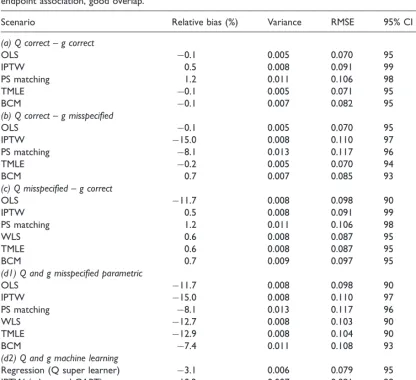
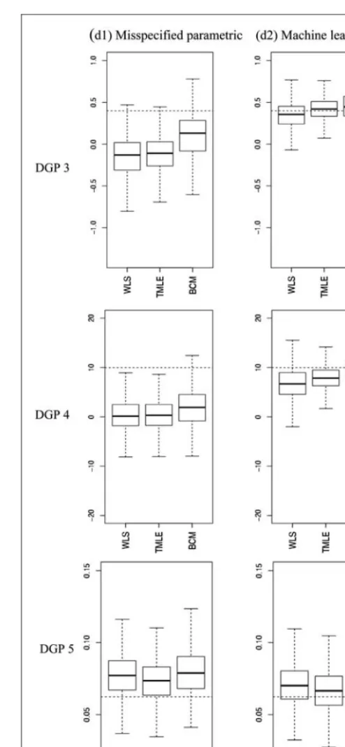
Tables 3 to 5 report the relative bias (%), variance, RMSE and 95% CI coverage for the estimators considered, and Figure 4 presents the distribution of the estimated ATEs with box plots.

Table 3 reports results for DGP 1, when there was good overlap, with a moderate association

between the confounders and a normally distributed endpoint. When both QðÞ and gðÞ were

(16)

method reported moderate levels of bias, but when machine learning estimation was used forQðÞ

andgðÞ, bias was reduced to close to zero for all the methods that combined these components, with WLS and TMLE providing estimates with the lowest RMSE.

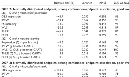
In DGP 2, with misspeciﬁed ﬁxed parametric methods, stronger association between the confounders and the endpoint led to higher biases, but with machine learning estimation the bias

for the methods that combined gðÞ and QðÞ was again below 10% (Table 4). WLS and TMLE

[image:16.592.68.485.93.473.2]

reported lower bias and RMSE than BCM. In DGPs 3–5, where there was poor overlap, with misspeciﬁed ﬁxed parametric models, each method reported high bias. For each of these DGPs, machine learning estimation improved performance of the methods that combined gðÞ and QðÞ.

Table 3. Simulation results for DGP 1, over 1000 replications: normal endpoint, moderate association confounder–

endpoint association, good overlap.

Scenario Relative bias (%) Variance RMSE 95% CI coverage (%)

(a) Q correct – g correct

OLS 0.1 0.005 0.070 95

IPTW 0.5 0.008 0.091 99

PS matching 1.2 0.011 0.106 98

TMLE 0.1 0.005 0.071 95

BCM 0.1 0.007 0.082 95

(b) Q correct – g misspecified

OLS 0.1 0.005 0.070 95

IPTW 15.0 0.008 0.110 97

PS matching 8.1 0.013 0.117 96

TMLE 0.2 0.005 0.070 94

BCM 0.7 0.007 0.085 93

(c) Q misspecified – g correct

OLS 11.7 0.008 0.098 90

IPTW 0.5 0.008 0.091 99

PS matching 1.2 0.011 0.106 98

WLS 0.6 0.008 0.087 95

TMLE 0.6 0.008 0.087 95

BCM 0.7 0.009 0.097 95

(d1) Q and g misspecified parametric

OLS 11.7 0.008 0.098 90

IPTW 15.0 0.008 0.110 97

PS matching 8.1 0.013 0.117 96

WLS 12.7 0.008 0.103 90

TMLE 12.9 0.008 0.104 90

BCM 7.4 0.011 0.108 93

(d2) Q and g machine learning

Regression (Q super learner) 3.1 0.006 0.079 95

IPTW (g boosted CART) 10.2 0.007 0.091 98

WLS (Q OLS, g boosted CART) 0.5 0.006 0.076 97

TMLE (Q SL, g boosted CART) 1.1 0.006 0.074 94

BCM (Q SL, g boosted CART) 2.1 0.008 0.092 95

(17)

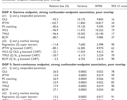
In DGP 3, TMLE provided the lowest bias and RMSE, albeit with CI coverage that was lower than the nominal level (Table 4). In DGP 4 where we considered an endpoint with a gamma distribution, with machine learning approaches BCM showed less relative bias (2.5%) and RMSE than TMLE (20.7%), however higher variance (Table 4). In DGP 5, where we considered an endpoint with a semi-continuous distribution, TMLE and BCM with machine learning estimation performed best; BCM gave the lowest relative bias (1.1% versus 7.2%) and best CI coverage whereas TMLE reported the lowest RMSE and variance (Table 5).

[image:17.592.50.472.106.359.2]

IPTW using machine learning weights often reported high bias: for example for DGP 5, it reported higher bias than using a misspecified, fixed logistic regression. This indicated that using boosted CARTs for estimating the PS was insufficient to eliminate bias. For DGPs 3–5, where overlap was poor, truncating the weights for IPTW and TMLE for either the logistic or the boosted PS models did not change the results.

Table 4. Simulation results for DGP 2 and 3, over 1000 replications: normal endpoint, strong confounder–endpoint

association, good and poor overlap.

Relative bias (%) Variance RMSE 95% CI coverage (%)

DGP 2: Normally distributed endpoint, strong confounder–endpoint association, good overlap

OLS regression 45.9 0.052 0.292 86

IPTW 59.1 0.067 0.350 98

PS matching 34.0 0.099 0.342 96

WLS 50.2 0.059 0.315 87

TMLE 45.7 0.041 0.272 86

BCM 31.4 0.074 0.299 90

DGP 3: Normally distributed endpoint, strong confounder–endpoint association, poor overlap

OLS regression 119.2 0.050 0.527 40

IPTW 160.6 0.082 0.703 71

PS matching 81.1 0.100 0.453 84

WLS 137.9 0.063 0.606 39

TMLE 129.7 0.046 0.561 35

BCM 73.8 0.072 0.399 74

(18)

5 Discussion

This paper ﬁnds that in circumstances when the parametric models for both the endpoint regression function and PS are misspeciﬁed, both TMLE and BCM can reduce bias when coupled with machine learning methods.

[image:18.592.62.491.95.432.2]

We considered these methods, alongside more traditional PS, regression and DR methods in a case study that evaluated the eﬀect of alternative types of THR for patients with osteoarthritis. This study illustrates a general challenge which is to specify a regression model for a non-normal endpoint (HRQoL), with a non-linear response surface. In the simulation studies, grounded in the case study, we generated endpoints data with normal, skewed and semi-continuous distributions, with non-linear covariate–endpoint relationships. In the simulated scenarios, where there was dual misspeciﬁcation, and machine learning techniques were used to estimate the endpoint

Table 5. Simulation results for DGP 4 and 5, over 1000 replications: Normal and gamma endpoints, strong

confounder–endpoint relationship, poor overlap.

Relative bias (%) Variance RMSE 95% CI coverage (%)

DGP 4: Gamma endpoint, strong confounder–endpoint association, poor overlap

OLS 93.3 10.175 9.843 16

IPTW 102.7 11.850 10.817 34

PS matching 85.6 19.120 9.595 59

WLS 96.9 11.475 10.252 19

TMLE 96.4 10.303 10.140 17

BCM 80.7 17.642 9.085 37

DGP 5: Semi-continuous endpoint, strong confounder–endpoint association, poor overlap

OLS 26.0 0.0002 0.022 78

IPTW 15.0 0.0003 0.019 99

PS matching 26.9 0.0004 0.026 93

WLS 23.9 0.0003 0.022 83

TMLE 17.9 0.0002 0.019 90

BCM 27.1 0.0003 0.024 82

(19)

[image:19.592.139.386.65.599.2]

(20)

regression function and the PS, both TMLE and BCM could greatly reduce bias, in contrast to the high bias where misspeciﬁed ﬁxed parametric models were used.

We found that the relative advantage of TMLE versus BCM was dependent on the features of the DGPs considered. In favourable settings such as good overlap and moderate association between the confounder and the endpoint, TMLE outperformed BCM in terms of bias and precision. This result corresponds to previous work that found that reweighting estimators outperformed BCM under good overlap.21 In a more challenging setting, when overlap was poor, and there was a strong association between the confounders and the endpoint, we found a bias–variance trade-oﬀ between the methods under comparison: for non-normal endpoints, BCM showed less bias, but was more variable than TMLE. We followed recent recommendations when reporting CIs for matching estimators,44 and like previous studies, we found that they reported somewhat higher than nominal coverage.20

Our work extends the previous literature in several aspects. First, this is the first paper that compares the relative performance of BCM and TMLE, and also compares these methods to traditional approaches. Second, while BCM has been proposed with flexible approaches for estimating the endpoint regression function, previous studies used OLS for adjustment.20,21 This study considers super learning, a machine learning method for bias correction, and finds that when matching is based on a PS that was also estimated using machine learning (boosted CARTs), the bias due to model misspecification was greatly reduced. We find this result across a range of DGPs including highly non-linear response surfaces. Third, unlike previous studies

that used machine learning only for selected combined methods such as TMLE,16 this paper

took a systematic approach and evaluated the impact of using machine learning estimation for single methods, such as regression and IPTW, and for combined methods, such as TMLE and BCM.

Similarly to Kang and Schafer (2007),12we find that combining the PS and endpoint regression from misspecified fixed parametric models does not reduce bias compared to using these models in single methods such as IPTW. In the scenarios considered in this study, it was the combined use of machine learning approaches for estimating the endpoint regression and the PS that helped eliminate most of the bias due to observed confounding.

This work has some caveats. The methods considered and the simulation settings all assume ‘no unobserved confounding’. Machine learning methods can augment but not necessarily replace subject-matter knowledge when selecting the set of confounders that need to be controlled for.76 In the case study, while we used a rich set of measured cofounders suggested by previous literature and clinical expert opinion,66some unobserved confounders such as unobserved patient preferences for prosthesis types may prevail. The scope of this paper did not extend to comparing alternative machine learning approaches. We found that boosted CARTs for estimating the PS, a method that has been found to outperform logistic regression and alternative machine learning approaches,24 did not consistently reduce bias compared to misspeciﬁed logistic regression. Further machine learning approaches may be considered for the PS, such as random forests24

or neural networks.8 These approaches also have promising application for estimating the

endpoint regression function.26 Any machine learning method relies on subjective choices of the user. For boosted CARTs, tuning parameters such as the shrinkage parameter needs to be selected.50

(21)

than relying on any one prediction algorithm. In the simulation study, in order to mimic a situation where the investigator does not know the true DGP, we required the super leaner to consider the same, restricted range of prediction algorithms (including GLMs, generalised additive models and multivariate adaptive polynomial spline regression) for each DGP. In practice, we recommend that the analyst requires the super learner to consider a richer set of prediction algorithms; a wide range of models and prediction algorithms should be proposed according to subject-matter knowledge to encourage the consistent estimation of the regression function albeit at the expense of increased computational time.39These prediction algorithms can include advanced model selection methods such as fractional polynomials77or penalised model selection approaches.78

This paper considered continuous and semi-continuous endpoints motivated by the case study. The approaches presented are in principle applicable to binary, count or survival outcomes and other parameters such as the odds ratio, risk ratio or hazard ratio. TMLE has been demonstrated to have good ﬁnite sample performance for binary and survival endpoints.17,59 While matching

estimators have also been proposed for estimating risk ratios and odds ratios,46,79 BCM

estimators for these parameters have not yet been developed.

In the simulations, each method is adjusted for the observed covariates known to be predictive of both treatment assignment and of the outcome. In practice, this feature of the DGP is not known, and subject-matter knowledge should be used to select for adjustment of those potential confounders that are measured before treatment, and are both predictive of treatment selection and the endpoint.1 The inclusion of those covariates which inﬂuence treatment assignment, but not the endpoint in the PS can lead to estimates that are statistically ineﬃcient.80–82

This work also opens up areas for future research. In the common settings of poor overlap, an extension of TMLE, collaborative maximum likelihood estimation (C-TMLE)55,83can outperform TMLE. C-TMLE uses machine learning to select a suﬃcient set of covariates for inclusion ingðÞ

that reduces bias while minimising overall mean squared error.

We conclude that both TMLE and BCM have the potential to reduce bias due to observed confounding, in common settings of dual misspeciﬁcation, if coupled with machine learning methods for estimating the PS and the endpoint regression function. TMLE is implemented as a readily available software package.61 For BCM, the available packages currently allow for regression adjustment using OLS only.62,84 In order to facilitate the uptake of the methods, the Supplementary Appendix provides code for the implementation of TMLE and BCM with machine learning.

Acknowledgements

We thank Jan vanderMeulen and Nick Black (LSHTM) for access to the PROMs data and the Department of Health for funding the primary analysis of the PROMs data. We are grateful to Mark Pennington (LSHTM) for advice on the motivating case study. We thank Rhian Daniel, Karla Diaz-Ordaz (LSHTM) and Adam Steventon (Nuﬃeld Trust) for valuable comments on the manuscript.

Funding

NK, RR and RG were funded by the Economic and Social Research Council (Grant no. RES-061-25-0343).

Conflict of interest

(22)

References

1. Rubin DB. On the limitations of comparative effectiveness research.Stat Med2010;29: 1991–1995.

2. Tunis SR, Benner J and McClellan M. Comparative effectiveness research: Policy context, methods development and research infrastructure.Stat Med2010;

29: 1963–1976.

3. Fung V, Brand RJ, Newhouse JP, et al. Using Medicare data for comparative effectiveness research: Opportunities and challenges.Am J Manag Care2011;17: 489–496. 4. Imbens GM and Wooldridge JM. Recent developments in

the econometrics of program evaluation.J Econ Lit2009;

47: 5–86.

5. Ho DE, Imai K, King G, et al. Matching as nonparametric preprocessing for reducing model dependence in parametric causal inference.Political Analysis2007;15: 199–236.

6. Basu A and Manca A. Regression estimators for generic health-related quality of life and quality-adjusted life years.

Med Decis Making, Epub ahead of print 18 October 2011. DOI: 10.1177/0272989X11416988.

7. Dehejia RH and Wahba S. Propensity score-matching methods for nonexperimental causal studies.Rev Econ Stat

2002;84: 151–161.

8. Westreich D, Lessler J and Funk M. Propensity score estimation: Neural networks, support vector machines, decision trees (CART), and meta-classifiers as alternatives to logistic regression.J Clin Epidemiol2010;63: 826–833. 9. Robins J, Rotnitzky A and Zhao LP. Estimation of

regression coefficients when some regressors are not always observed.J Am Stat Assoc1994;89: 846–866. 10. Robins J, Sued M, Lei-Gomez Q, et al. Comment:

Performance of double-robust estimators when ‘‘inverse probability’’ weights are highly variable.Stat Sci2007;22: 544–559.

11. Westreich D and Cole SR. Invited commentary: Positivity in practice.Am J Epidemiol2010;171: 674–677. 12. Kang JDY and Schafer JL. Demystifying double

robustness: A comparison of alternative strategies for estimating a population mean from incomplete data.Stat Sci2007;22: 523–539.

13. Freedman D and Berk RA. Weighting regression by propensity score.Eval Rev2008;32: 392–409. 14. van der Laan MJ. Targeted maximum likelihood based

causal inference: Part I.Int J Biostat2010;6: 1–42. DOI: 10.2202/1557-4679.1211.

15. van der Laan MJ and Rubin D. Targeted maximum likelihood learning. U.C. Berkeley Division of Biostatistics Working Paper Series. Working Paper 213, October 2006, http://biostats.bepress.com/ucbbiostat/paper213. 16. Porter KE, Gruber S, van der Laan MJ, et al. The relative

performance of targeted maximum likelihood estimators.

Int J Biostat2011;7: 1–34. DOI: 10.2202/1557-4679.1308. 17. Stitelman OM and van der Laan MJ. Collaborative

targeted maximum likelihood for time to event data.Int J Biostat2010;6: 1–46.

18. Gruber S and van der Laan M. A targeted maximum likelihood estimator of a causal effect on a bounded continuous outcome.Int J Biostat2010;6: Article 26. DOI: 10.2202/1557-4679.1260.

19. Rubin DB. The use of matched sampling and regression adjustment to remove bias in observational studies.

Biometrics1973;29: 185–203.

20. Abadie A and Imbens GW. Bias-corrected matching estimators for average treatment effects.J Bus Econ Stat

2011;29: 1–11.

21. Busso M, DiNardo J and McCrary J. New evidence on the finite sample properties of propensity score reweighting and matching estimators, 2011. Contract No. 3998.

22. Rubin DB and Thomas N. Combining propensity score matching with additional adjustments for prognostic covariates.J Am Stat Assoc2000;95: 573–585. 23. Rubin DB. Using multivariate matched sampling and

regression adjustment to control bias in observational studies.J Am Stat Assoc1979;74: 318–328.

24. Lee BK, Lessler J and Stuart EA. Improving propensity score weighting using machine learning.Stat Med2010;29: 337–346.

25. Setoguchi S, Schneeweiss S, Brookhart M, et al. Evaluating uses of data mining techniques in propensity score estimation: A simulation study.Pharmacoepidemiol Drug Saf2008;17: 546–555.

26. Austin PC. Using ensemble-based methods for directly estimating causal effects: An investigation of tree-based G-computation.Multivar Behav Res2012;47: 115–135. 27. Ridgeway G and McCaffrey DF. Comment: Demystifying

double robustness: A comparison of alternative strategies for estimating a population mean from incomplete data.

Stat Sci2007;22: 540–543.

28. Austin PC. A critical appraisal of propensity-score matching in the medical literature between 1996 and 2003.

Stat Med2008;27: 2037–2049.

29. Caliendo M and Kopeinig S. Some practical guidance for the implementation of propensity score matching.J Econ Surv2008;22: 31–72.

30. PROMs.Provisional Monthly Patient Reported Outcome Measures (PROMs) in England. April 2009–April 2010: Pre- and post-operative data: Experimental statistics.The Health and Social Care Information Centre, 2010. 31. Ousey K and Cook L. Understanding patient reported

outcome measures (PROMs).Br J Commun Nurs2011;16: 80–82.

32. Greenland S, Pearl J and Robins JM. Confounding and collapsibility in causal inference.Stat Sci1999;14: 29–46. 33. Cole SR and Frangakis CE. The consistency statement in

causal inference: A definition or an assumption?

Epidemiology2009;20: 3–5.

34. Imbens GW. Nonparametric estimation of average treatment effects under exogeneity: A review.Rev Econ Stat2004;86: 4–29.

35. Robins J. A new approach to causal inference in mortality studies with a sustained exposure period – application to control of the healthy worker survivor effect.Math Modelling1986;7: 1393–1512.

36. Imbens G and Wooldridge JM.New developments in econometrics.Lecture Notes, CEMMAP, UCL2009b. 37. Rubin DB. Estimating causal effects from large data sets

using propensity scores.Ann Intern Med1997;127: 757–763. 38. van der Laan MJ, Polley EC and Hubbard AE. Super

learner.Stat Appl Genet Mol Biol2007;6. DOI: 10.2202/ 1544-6115.1309.

39. Polley EC and van der Laan MJ. Super Learner in prediction. U.C. Berkeley Division of Biostatistics Working Paper Series. Working Paper 266, May 2010, http://biostats.bepress.com/ucbbiostat/paper266. 40. van der Laan MJ and Dudoit S. Unified cross-validation

methodology for selection among estimators and a general cross-validated adaptive epsilon-net estimator: Finite sample oracle inequalities and examples. U.C. Berkeley Division of Biostatistics Working Paper Series. Working Paper 130, November 2003, http://biostats.bepress.com/ ucbbiostat/paper130.

41. Rosenbaum PR and Rubin DB. The central role of the propensity score in observational studies for causal effects.

Biometrika1983;70: 41–55.

(23)

on right heart catheterization.Health Serv Outcomes Res Methodol2001;2: 259–278.

43. Waernbaum I. Model misspecification and robustness in causal inference: Comparing matching with doubly robust estimation.Stat Med2011;31: 1572–1581.

44. Abadie A and Imbens GW. Large sample properties of matching estimators for average treatment effects.

Econometrica2006;74: 235–267.

45. Hirano K, Imbens GW and Ridder G. Efficient estimation of average treatment effects using the estimated propensity score.Econometrica2003;71: 1161–1189.

46. Radice R, Grieve R, Ramsahai R, et al. Evaluating treatment effectiveness in patient subgroups: A comparison of propensity score methods with an automated matching approach.Int J Biostat2012;8: 1–43. 47. Cole SR and Herna´n MA. Constructing inverse

probability weights for marginal structural models.Am J Epidemiol2008;168: 656–664.

48. Elliott MR. Model averaging methods for weight trimming.J Off Stat2008;24: 517–540.

49. Crump RK, Hotz VJ, Imbens GW, et al. Dealing with limited overlap in estimation of average treatment effects.

Biometrika2009;96: 187–199.

50. McCaffrey D, Ridgeway G and Morral A. Propensity score estimation with boosted regression for evaluating causal effects in observational studies.Psychol Methods

2004;9: 403–425.

51. Stuart EA. Matching methods for causal inference: A review and a look forward.Stat Sci2010;25: 1–144. 52. Bang H and Robins JM. Doubly robust estimation in

missing data and causal inference models.Biometrics2005;

61: 962–972.

53. Kang JDY and Schafer JL. Rejoinder: Demystifying double robustness: A comparison of alternative strategies for estimating a population mean from incomplete data.

Stat Sci2007;22: 574–580.

54. Basu A, Polsky D and Manning W. Estimating treatment effects on healthcare costs under exogeneity: Is there a ‘magic bullet’?Health Serv Outcomes Res Methodol2011;11: 1–26. 55. van der Laan MJ and Gruber S. Collaborative double

robust targeted maximum likelihood estimation.Int J Biostat2010;6: 1–68. DOI: 10.2202/1557-4679.1181. 56. Gudex C, Kind P and Williams A. A social tariff for

EuroQol: results from a UK general population survey. Centre for Health Economics, University of York, 1995, pp. 1–24.

57. Rotnitzky A, Lei Q, Sued M, et al. Improved double-robust estimation in missing data and causal inference models.Biometrika2012;99: 439–456.

58. Gruber S and van der Laan MJ. Targeted minimum loss based estimation of causal effects on an outcome with known conditional bounds.Int J Biostat2012;8. DOI: 10.1515/1557-4679.1370.

59. Moore KL and van der Laan MJ. Covariate adjustment in randomized trials with binary outcomes: Targeted maximum likelihood estimation.Stat Med2009;28: 39–64. 60. Hampel FR. The influence curve and its role in robust

estimation.J Am Stat Assoc1974;69: 383–393. 61. Gruber S and van der Laan MJ. tmle: An R package for

targeted maximum likelihood estimation.J Stat Software

2012;51: 1–35.

62. Abadie A, Herr JL, Imbens GW, et al. NNMATCH: Stata module to compute nearest-neighbor bias-corrected estimators. Chestnut Hill, MA, USA: Boston College Department of Economics, 2004, http://fmwww.bc.edu/ repec/bocode/n/nnmatch.hlp.

63. Austin PC. Statistical criteria for selecting the optimal number of untreated subjects matched to each treated subject when using many-to-one matching on the propensity score.Am J Epidemiol2010;172: 1092–1097.

64. NICE. Health Technology Appraisal. Total hip replacement and resurfacing arthroplasty for the treatment of pain or disability resulting from end stage arthritis of the hip (Review of technology appraisal guidance 2 and 44). Final scope, 2012, http://www.nice.org.uk/nicemedia/ live/13690/61348/61348.pdf (accessed 31 July 2012). 65. EuroQol Group. EuroQol—a new facility for the

measurement of health-related quality of life.Health Policy1990;16: 199–208.

66. Pennington M, Grieve R, Sekhon JS, et al. Cemented, cementless and hybrid prostheses for total hip

replacement: A cost-effectiveness analysis.Br Med J2013;

346: f1026. DOI: 10.1136/bmj.f1026.

67. Carpenter J and Kenward M.Multiple imputation and its application. John Wiley & Sons, 2012.

68. Rubin D. Multiple imputation after 18þyears.J Am Stat Assoc1996;91: 473–489.

69. Tooze JA, Grunwald GK and Jones RH. Analysis of repeated measures data with clumping at zero.Stat Methods Med Res2002;11: 341–355.

70. Buntin MB and Zaslavsky AM. Too much ado about two-part models and transformation?: Comparing methods of modeling Medicare expenditures.J Health Econ2004;23: 525–542.

71. R Development Core Team.R: A language and environment for statistical computing.Vienna, Austria: R Foundation for Statistical Computing, 2011.

72. Polley EC and van der Laan MJ. R package ‘‘SuperLearner’’, 2010, http://cran.r-project.org/web/ packages/SuperLearner/index.html (accessed 15 June 2012).

73. Kooperberg C. Polspline: Polynomial spline routines, 2010 CRAN, Software Package, http://cran.r-project.org/web/ packages/polspline/ (accessed 15 June 2012).

74. Ridgeway G, McCaffrey D, Morral A, et al. twang: Toolkit for weighting and analysis of nonequivalent groups. CRAN, Software Package, http://cran.r-project.org/web/packages/twang/index.html.

75. Davison A and Hinkley D.Bootstrap methods and their application. New York: Cambridge University Press, 1997. 76. Rubin DB. The design versus the analysis of observational

studies for causal effects: Parallels with the design of randomized trials.Stat Med2007;26: 20–36. 77. Sauerbrei W, Royston P and Binder H. Selection of

important variables and determination of functional form for continuous predictors in multivariable model building.

Stat Med2007;26: 5512–5528.

78. Fan J and Li R. Variable selection via nonconcave penalized likelihood and its oracle properties.J Am Stat Assoc2001;96: 1348–1360.

79. Austin PC. The performance of different propensity score methods for estimating marginal odds ratios.Stat Med

2013;32: 2837–2849.

80. Brookhart MA, Schneeweiss S, Rothman KJ, et al. Variable selection for propensity score models.Am J Epidemiol2006;163: 1149–1156.

81. Senn S, Graf E and Caputo A. Stratification for the propensity score compared with linear regression techniques to assess the effect of treatment or exposure.

Stat Med2007;26: 5529–5544.

82. Guo H and Dawid AP (eds). Sufficient covariates and linear propensity analysis. In:International conference on artificial intelligence and statistics, 2010, pp. 281–288. 83. Gruber S and van der Laan MJ. An application of

collaborative targeted maximum likelihood estimation in causal inference and genomics.Int J Biostat2010;6: 1–29. DOI: 10.2202/1557-4679.1182.

84. Sekhon JS. Matching: Multivariate and propensity score matching with automated balance search.J Stat Software