Spatial heterodyne spectroscopy: Modeling and interferogram processing

(1)

Rochester Institute of Technology

RIT Scholar Works

Theses

Thesis/Dissertation Collections

7-29-2013

Spatial heterodyne spectroscopy: Modeling and

interferogram processing

Cara Perkins

Follow this and additional works at:

http://scholarworks.rit.edu/theses

Recommended Citation

(2)

Spatial Heterodyne Spectroscopy: Modeling and Interferogram

Processing

by

Cara P. Perkins

B.S. Merrimack College, 2011

A thesis submitted in partial fulfillment of the requirements for the degree of Master of Science in the Chester F. Carlson Center for Imaging Science

of the College of Science Rochester Institute of Technology

July 29, 2013

Signature of the Author

Accepted by

(3)

CHESTER F. CARLSON CENTER FOR IMAGING SCIENCE COLLEGE OF SCIENCE

ROCHESTER INSTITUTE OF TECHNOLOGY ROCHESTER, NEW YORK

CERTIFICATE OF APPROVAL

M.S. DEGREE THESIS

The M.S. Degree Thesis of Cara P. Perkins has been examined and approved by the

thesis committee as satisfactory for the thesis required for the

M.S. degree in Imaging Science

Dr. John Kerekes, Thesis Advisor

Dr. Michael Gartley

Dr. Carl Salvaggio

(4)

Spatial Heterodyne Spectroscopy: Modeling and Interferogram

Processing

by Cara P. Perkins

Submitted to the

Chester F. Carlson Center for Imaging Science College of Science

in partial fulfillment of the requirements for the Master of Science Degree at the Rochester Institute of Technology

Abstract

This work presents a radiometric model of a spatial heterodyne spectrometer (SHS) and a corresponding interferogram-processing algorithm for the calculation of calibrated spectral radiance measurements. The SHS relies on Fourier Transform Spectroscopy (FTS) principles, and shares design similarities with the Michelson Interferometer. The advantages of the SHS design, including the lack of moving parts, high throughput, and instantaneous spectral measurements, make it suitable as a field-deployable instrument. Operating in the long-wave infrared (LWIR), the imaging SHS design example included provides the capability of performing chemical detection based on reflectance and emissivity properties of surfaces of organic compounds.

This LWIR SHS model takes into account the instruments entrance optics, interferome-ter, exit optics, and detection scheme to output realistic, interferometric data. The model serves as a tool to find the optimal SHS design parameters for the desired performance requirements and system application. It also assists in the data analysis and system characterization.

(5)

Acknowledgements

Firstly, I would like to thank my thesis advisor, Dr. John Kerekes, for all his assistance and support and, of course, research funding. My career at the Center for Imaging Science (CIS) followed an unusual path and if it had not been for Dr. Kerekes, I would probably still be trying to figure out what my thesis topic is. I would also like to thank my thesis committee members, Dr. Michael Gartley for his advice on qualitative measurement comparisons and Dr. Carl Salvaggio for the use of his course lectures and his SHS model suggestions.

Thank you to Dr. Mar´ıa Helguera, who persuaded me to pursue my graduate career in imaging science and welcomed me as a part of her laboratory. Though our circumstances did not afford for us to work together, I am very appreciative for all her advice and encouragement along the way.

Finally, I would like to say thank you to all my friends and family, who have never once doubted me, and especially to Kyle for always listening to me babble.

(6)

(7)

List of Figures

3.1 A dispersive spectrometer that uses prisms relies on Snell’s law to disperse incoming light into its separate wavelength components [1]. . . 6 3.2 A diffraction grating disperses the incoming light beam into its separated

wavelength constituents. Here, λ1 6=λ2 6=λ3 [2]. . . 6

3.3 The MI separates incoming light into two beams using a beam-splitter. Each beam travels the length of one of the interferometer arms, reflects off the mirror, and recombines with the other at the detector [3]. . . 9 3.4 The two monochromatic wave-fronts from the two interferometer arms

recombine at the focal plane array (A.) and create the interference fringe pattern (B.). One row of the fringe pattern gives us the interferogram (C.) [4]. 10 3.5 The Sagnac Interferometer usually consists of a beam splitter and three

mirrors. The two, separated light beams travel to each mirror before reaching the detector, but in opposite directions. A beam-splitter tilt angle creates a phase difference between the two, recombining beams, creating the interference pattern [5]. . . 11 3.6 The Fabry-Perot Interferometer usually consists of two highly reflective

plates that face each other. Incoming light is reflected and transmitted each time it is incident on a plate [6]. . . 12 3.7 The Fabry-Perot interferometer produces a non-sinusoidal signal. Unlike

that of the MI, the IFT of this signal gives the source spectrum contaminated with harmonics [7]. . . 14 3.8 The SHS (B.) design is almost identical to that of the MI (A.). The main

difference is that the mirrors in the MI are replaced by diffraction gratings tilted by the Littrow angle in the SHS [4]. . . 15 3.9 One diffraction grating, G1, in the SHS. The z-axis runs parallel to the

(12)

LIST OF FIGURES xi

3.10 By means of an anamorphic telescope, the SHS can collect rows or columns of pixels at a time, recording the spatial information in one dimension of the detector and spectral information in the other dimension. After scanning for a desired number of rows or columns, the result is a complete hyperspectral data cube [9]. . . 20 4.1 FIRST by Telops is an imaging Michelson interferometer operating in the

LWIR. Depicted here is the interferometer subsystem [10]. . . 22 4.2 The LIFTIRS collection time is approximately twice that of the FIRST

collection time while using the same image size and spectral resolution [11]. 23 4.3 The THI uses a Sagnac interferometer to collect HSI at a spectral resolution

of about 16cm−1 _{[12]. . . .} ₂₄

4.4 The AIRIS is a tunable Fabry-Perot interferometer with built-in hot and cold blackbodies for internal calibration [13]. . . 24 4.5 The IRISHS uses an IR SHS with a FPA to record an image of the sampled

scene and an interferogram for each pixel in the image [4]. . . 25 4.6 SHIMCAD is an imaging IR SHS like IRISHS, using an anamorphic telescope

to image the scene onto the SHS aperture and a FPA to collect the scene’s spatial and spectral information [14]. . . 26 5.1 The RECT function has unit amplitude between−xmax and xmax [15]. . . . 34

5.2 The SINC function has a center peak with oscillations on either side that eventually go to zero amplitude [16]. . . 35 5.3 The first column shows common apodization functions, the second column

shows their FT’s, and the last column shows a magnified view of their side lobes [17]. . . 38 6.1 The entire SHS system consists of the input, or the scene spectral radiance,

the SHS itself, and processing software to determine the measured spectral radiance. . . 40 6.2 Cooke et. al’s model accepts the sample radiance with added background

radiance. The input undergoes the entrance optics, Optics I, the SHS configuration, Interferometer, the exit optics, Optics II, and the detection scheme (Field-Stop, Filter, FPA, and Cold Shield) [4]. . . 40 7.1 Results of the MODTRAN test: in clockwise rotation from top left, the

(13)

7.2 Results of the recorded sand test: in clockwise rotation from top left, the input atmospheric spectral radiance spectrum, measured interferogram, wavenumber-dependent SNR, shift-corrected interferogram, recovered spec-trum, and wavenumber-dependent NEdT. . . 49 7.3 Results of the simulated sand test: in clockwise rotation from top left,

the input atmospheric spectral radiance spectrum, measured interferogram, wavenumber-dependent SNR, shift-corrected interferogram, recovered spec-trum, and wavenumber-dependent NEdT. . . 50 7.4 Results of the system trade-off between spectral range and spectral resolution. 50 7.5 Results of the system trade-off between diffraction grating width and spectral

resolution. . . 51 7.6 Results of the system trade-off between throughput and SNR. . . 51 7.7 Results of the Littrow angle error, clockwise from top left: RMSE, percent

accuracy, SDR, and separation angle. . . 53 7.8 Results of the phase error, clockwise from top left: RMSE, percent accuracy,

SDR, and separation angle. . . 54 7.9 Results of the calibration error rate, clockwise from top left: RMSE, percent

accuracy, SDR, and separation angle. . . 55 7.10 Results of the detector position error, clockwise from top left: RMSE, percent

accuracy, SDR, and separation angle. . . 56 7.11 Results of the average spectrum recovery percent accuracy as a function of

SNR. . . 57 7.12 Results of the methanol (93.3 hPa) test at 128 samples: in clockwise rotation

from top left, the input methanol gas transmittance spectrum, measured interferogram, wavenumber-dependent SNR, shift-corrected interferogram, recovered spectrum, and wavenumber-dependent NEdT. . . 58 7.13 Results of the SHIMCAD measurement of methanol transmittance (59.9 hPa). 58 7.14 Results of the methanol (93.3 hPa) test at 256 samples: in clockwise rotation

from top left, the input methanol gas transmittance spectrum, measured interferogram, wavenumber-dependent SNR, shift-corrected interferogram, recovered spectrum, and wavenumber-dependent NEdT. . . 59 9.1 A depiction of the field-widened SHS with prisms placed between the

diffrac-tion gratings and beam-splitter [18]. . . 62 B.1 There are three system folders. SHS contains code to generate

(14)

LIST OF FIGURES xiii

(15)

List of Tables

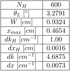
7.1 The user-specified operational parameters for the LWIR SHS design example. 46 7.2 The additional parameters calculated by the SHS model using the

user-specified operational parameters. . . 46

A.1 Summary of Interferometer Technologies . . . 64

C.1 Summary of Comparison . . . 112

(16)

Chapter 1

Introduction

Fourier Transform Spectrometers (FTS) have long been used to measure a sample’s spectrum [3, 19, 20, 21, 22]. The main advantage of the FTS over typical dispersive spec-trometers, which use either diffraction gratings or prisms to separate incoming wavenumbers, is that it does not require the use of an entrance slit. Rather, it uses a wide, circular aperture. The term, optical throughput, is used to describe the amount of space through which light can enter an optical system. The large aperture of the FTS, as compared to the thin entrance slit of the dispersive spectrometer, provides a much higher optical throughput, allowing much more radiant energy to enter and, thus, increasing the signal-to-noise ratio. A specific FTS, the Spatial Heterodyne Spectrometer (SHS) is known for having a very high throughput and is, therefore, often used to study emission lines [23, 24]. An SHS is very similar to a Michelson Interferometer (MI), a very well-known FTS [3]. A MI uses a beam-splitter to divide the incoming light into two interferometer arms, each containing a mirror to reflect the light to be recombined. After the separated wavefronts recombine at the detector, we have interference as a function of the difference in the optical path length of the two, separated beams. One mirrored-arm moves in increments to measure the interference at each optical path-length difference (OPD) within the system range. An SHS also uses a beam-splitter, but both its interferometer arms are fixed and contain diffraction gratings in place of mirrors, causing wavenumber-dependent tilts. The SHS design collects interference measurements at each OPD simultaneously and without any moving parts, making it more compact and robust [25].

(17)

Naval Research Laboratory has designed the first and, currently, the only, successful LWIR SHS [14].

(18)

Chapter 2

Project Overview

2.1

Research Goals

Because LWIR SHS theory is rather understudied, this thesis will provide two tools to assist with design optimization and characterization and data analysis. Possible instrument design parameters and assumptions will be used to model the LWIR SHS and generate raw interferograms. An interferogram processing algorithm will also be developed to convert the raw interferograms to calibrated radiance spectra. The model serves as a decision tool for SHS design parameters and system and performance analysis tool for any SHS design. The processing algorithm may also be applied to a wide variety of SHS systems.

2.2

Objectives

The objectives of this thesis are:

1. to create a model of a realistic SHS for generating raw interferograms,

2. to design an interferogram processing algorithm for converting SHS interferograms into calibrated radiance spectra with real-time capability,

3. to demonstrate design optimization and system characterization using the results of (1) and (2), and

(19)

2.3

Contributions to Knowledge

(20)

Chapter 3

Background

3.1

Spectroscopy

Spectral information has been used to determine material composition for many years. Some of the simplest tools for studying objects’ spectra are dispersive spectrometers. A dispersive spectrometer measures the spectrum of a source by separating the incoming radiation into its different spectral components, using a prism (see Figure 3.1) or diffraction grating (see Figure 3.2) to bend the light as a function of wavelength. The sensor is made of one detector element that is moved to view the spectral components individually or an array of detector elements to view all the components at once [20].

A prism relies on the wavelength-dependent refractive index of a material and Snell’s law:

n1(λ) sinθ1 =n2(λ) sinθ2, (3.1)

wheren1(λ) and n2(λ) are the refractive indices of the first and second material the light

passes through, respectively,λis the wavelength of light, andθ1 and θ2 are the incident

and refracted angles of the light, respectively, with respect to the normal of the surface of the second material.

A diffraction grating derives the spectrum by: 1

λ[sin (θ1) + sin (θ2)] =m/d, m= 0,±1,±2, ... (3.2) whereθ1andθ2are the incident and refracted angles of the light, respectively,mis the order

of diffraction, anddis the distance between the grating grooves. Constructive interference for a given wavelength occurs at integer values ofm, while destructive interference occurs at half-integer values ofm.

The value of θ2 depends on wavelength, such that the diffraction grating separates

(21)

[image:21.612.157.450.89.289.2]

Figure 3.1: A dispersive spectrometer that uses prisms relies on Snell’s law to disperse incoming light into its separate wavelength components [1].

Figure 3.2: A diffraction grating disperses the incoming light beam into its separated wavelength constituents. Here, λ1 6=λ26=λ3 [2].

(22)

3.2

Optical Throughput

Optical throughput, sometimes called etendue, describes the space through which light may enter an optical system. Throughput is defined by:

GE =AaΩa, (3.3)

where Aa is the area of the aperture and Ωa is the field-of-view (FOV) subtended by the

system aperture determined by the spectral resolving power,R:

Ωa=

2π

R, (3.4)

A larger system aperture or FOV will provide a greater optical throughput, allowing more light energy to enter the system. A high optical throughput is desirable because it increases the system sensitivity, therefore increasing the signal-to-noise ratio (SNR). In many optical systems, there is a trade-off between the optical throughput and the system resolution. For example, the dispersive spectrometer requires a rather narrow entrance slit to achieve a usable spectral resolution, but this creates a low optical throughput, decreasing system sensitivity and overall SNR.

3.3

Interferometry

Interferometry is a broad term used to describe any technique in which electromagnetic waves undergo interference in order to extract information about a radiant energy source. The tool used to cause the light interference is the interferometer.

3.3.1 Fourier Transform Spectroscopy

A very large family of interferometers exist. Of concern in this research is the subset of interferometers called Fourier Transform Spectrometers (FTS). As is explained in the following sections, a FTS measures a horizontal row of the interference pattern it creates from the input light beam. This measurement is the real part of the Fourier Transform (FT) of the source spectrum.

Both the dispersive spectrometer and the FTS can be used to measure a source spectrum. The FTS has the following advantages over the dispersive spectrometer:

(23)

• Connes Advantage: The FTS has a built-in HeNe laser for self-calibration [21]

3.3.2 Michelson Interferometer

The Michelson interferometer (MI) belongs to the FTS family. It consists of two interferometer arms and a beam-splitter to create two, separate wavefronts to travel down each of its arms (see Figure 3.3). Each beam travels along its respective path, reflects off the mirror at the end of the interferometer arm, and recombines with the other reflected beam at the sensor, creating part of the interference pattern. One mirror is moved to change the path length of one of the beams with respect to the other. The difference between the total lengths traveled by each beam is known as the optical path difference (OPD):

OP D =l2−l1, (3.5)

where l1 and l2 are the lengths of the travel paths in the first and second MI arms,

respectively. The OPD between the recombining beams determines the phase difference between the two. The phase difference then determines the coherence of the interfering beams. For a monochromatic source, the phase difference between the two reflected beams is given by:

∆φ= 2πOP D

λ . (3.6)

If

∆φ=±2(m+ 1)π, where m= 0,±1,±2, etc., (3.7) then the recombining beams are completely coherent and there is constructive interference. If

∆φ= 2mπ, m= 0,1,2, etc., (3.8) then the recombining beams are completely decoherent and there is destructive interference [3].

3.3.3 Interferogram Basics

The output signal of an interferometer, called an interferogram, is a single row of the interference pattern produced by the recombining wave-fronts at the detector. The interferogram is a measurement of intensity as a function of OPD, consisting of information from all the contributing frequencies in the input signal [21].

If we consider the interference of two wave-fronts with wave-vectors, k~1 andk~2, we can

(24)

Figure 3.3: The MI separates incoming light into two beams using a beam-splitter. Each beam travels the length of one of the interferometer arms, reflects off the mirror, and recombines with the other at the detector [3].

I =I1+I2+ 2

p

I1I2cos [~r·(k~1−k~2) + (φ1−φ2)], (3.9)

whereI1 andI2 are the intensity magnitudes andφ1 andφ2 are the phases of the

wave-fronts corresponding tok~1 and k~2, respectively. If I1 =I2 (as is true in the interferometer

since the two interfering beams are from the same source) andφ1=φ2 = 0, then

I = 2I1(1 + cos [~r·(k~1−k~2)][8]. (3.10)

Specifically, the cosine argument is the phase difference between the two waves recombining at the detector. Using Equation 3.6:

I(OP D) = 1

2L(k)[1 + cos (2πk·OP D)], (3.11) wherek is the wavenumber:

k= 1

λ (3.12)

(25)

Figure 3.4: The two monochromatic wave-fronts from the two interferometer arms recombine at the focal plane array (A.) and create the interference fringe pattern (B.). One row of the fringe pattern gives us the interferogram (C.) [4].

other part is not. The modulated portion of the signal is what provides the interferogram, by definition:

I(OP D) = 1/2·L(k) cos (2πk·OP D) (3.13) The above equation is for the ideal interferogram of a monochromatic source. A more realistic equation takes into account the reflection and transmission coefficients and self-emission of the internal optics (i.e. the beam-splitter and mirrors). We will describe this in more detail in Section 6.1. For a polychromatic source, the interferogram equation becomes:

I(OP D) =

Z ∞

−∞

1/2·L(k) cos (2πk·OP D)dk. (3.14)

The cosine term in the interferogram equation indicates that the interferogram is, essentially, a cosine transform (or the real part of the Fourier transform) of L(k). To obtain the spectral radiance of the source, L(k), we take the inverse Fourier Transform (IFT) of I(OP D):

L(k) =

Z ∞

−∞

(26)

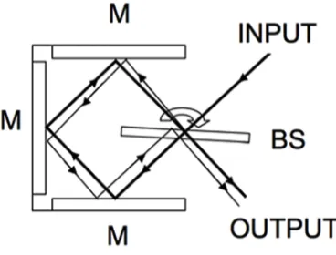
3.3.4 Sagnac Interferometer

Similar to the Michelson interferometer, the Sagnac interferometer divides the incoming light into two beams with a beam-splitter. Consider one common Sagnac interferometer geometry in Figure 3.5. One beam travels to the first, second, and third mirrors before the detector. The other beam travels to the third, second, and first mirrors before the detector. As implied in Figure 3.5, introducing a beam-splitter tilt angle, ∆θ, will create a phase difference between the two beams at the detector because each beam travels a slightly different path. The OPD in this Sagnac interferometer then becomes:

OP D= 4x∆θ, (3.16)

wherex is the position along the detector. Substituting Equation 3.16 into Equation 3.11 gives the interferogram equation for the Sagnac interferometer for a monochromatic source:

[image:26.612.213.397.382.522.2]

I(x) =L(k)[1 + cos (2πk·4x∆θ)]. (3.17) From Equation 3.16, we see that the OPD is a function of x, meaning that the Sagnac interferometer collects the interference pattern spatially rather than temporally as in the MI. As we will soon see, the SHS also collects an interferogram spatially, but with a higher spectral resolution.

(27)

Figure 3.6: The Fabry-Perot Interferometer usually consists of two highly reflective plates that face each other. Incoming light is reflected and transmitted each time it is incident on a plate [6].

3.3.5 Fabry-Perot Interferometer

Unlike the Michelson and Sagnac, the Fabry-Perot interferometer (FPI) is not, ordinarily, a FTS. The Fabry-Perot interferometer, as shown in Figure 3.6, consists of two parallel plates with highly reflecting surfaces that face each other. When light enters the area between the two plates, some of it is transmitted and some of it is reflected at each air-plate interface. Each reflection exhibited by a beam experiences a phase shift of:

∆φ= 4πk·ndcosθ, (3.18)

where nis the index of refraction of the medium between the two reflective plates, dis the distance between the plates, andOP D= 2dcosθ. The wavenumber-dependent phase difference between the transmitted beams causes an interference pattern, consisting of rings, known as Newton’s rings [29]. Sometimes, one thick plate with two reflecting surfaces is used in place of a pair of parallel reflecting plates. This device is more often called a Fabry-Perot etalon.

The total transmittance function of a Fabry-Perot instrument is:

τF P =

(1−r)2 1 +r2₋_2r_{cos ∆φ}

= 1

(1 +fsin2_(∆φ/2)),

(28)

where r is the reflectance of the parallel plates or surfaces of the etalon plate, and f is the Fabry-Perot coefficient of finesse:

f = 4r

(1−r)2. (3.20)

The quantity of finesse describes the sharpness of the etalons transmission peaks (i.e. the resolution) and is defined by:

F = π

2 sin−1(1/√f) ≈π/2

p

f[30]. (3.21)

The output of the FPI is then a series of narrow transmission bands:

It=I0

1 1 +₍₁₋4r_r₎2sin2(2πk·

OP D

2 )

[29], (3.22)

where I0 is the input beam intensity. Varying the plate separation distance, d, allows for

the collection of intensity as a function of OPD, as in the MI.

3.3.6 Fabry-Perot Interferometer as a Fourier Transform Spectrometer

As mentioned in the previous section, the output of an FPI with highly reflecting plates is a pattern of Newton’s rings (i.e. an Airy function). Meanwhile, the output of an MI is a cosine function. Performing an IFT on the output of the MI gives a single peak at a particular wavenumber for a monochromatic source. The IFT for the output of the FPI for that same source is a series of peaks. In other words, because the output of the FPI is not purely sinusoidal, the IFT of its output gives us a contaminated spectrum - the spectrum of the source and its harmonics. This concept is demonstrated in Figure 3.7.

Previous studies [29, 31], however, have demonstrated that the FPI can operate as a FTS. If the reflectance of the plates in the FPI is low, Equation 3.22 becomes:

It=I0

1

1 +₍₁₋4r_r₎2sin2(2πk·OP D)

≈I0(1−

4r (1−r)2sin

2_(2πk_·_{OP D))}

=I0(

4r 2(1−r)2 −

4r

2(1−r)2 cos (4πk·OP D)).

(3.23)

(29)

Figure 3.7: The Fabry-Perot interferometer produces a non-sinusoidal signal. Unlike that of the MI, the IFT of this signal gives the source spectrum contaminated with harmonics [7].

3.4

Spatial Heterodyne Spectroscopy

The spatial heterodyne spectrometer (SHS) is another type of interferometer that falls into the FTS category. The SHS is similar in design to the MI, but with diffraction gratings in place of mirrors in the arms (see Figure 3.8). Each diffraction grating creates a wave-front at a wavenumber-dependent spatial frequency, separated by a wavenumber-dependent angle for each wavenumber in the input beam. When the two wave-fronts recombine at the detector, they create interference fringes, known as Fizeau fringes, and represent the FT of the source’s spectrum about the heterodyne wavenumber. The heterodyne wavenumber is that which produces parallel wave-fronts (i.e. the separation angle is zero) with zero spatial frequency, and is known as the Littrow wavenumber. The diffraction gratings allow us to create the entire interference pattern and record the interferogram without moving any interferometer parts [25].

Like dispersive spectrometers, the SHS uses diffraction gratings to separate the wave-fronts by their spatial frequencies. However, as noted above, FTS instruments have a much higher throughput - about 200 times larger than that of a conventional dispersive spectrometer [21] due to their circular apertures. In addition to the advantages of FTS listed in Section 3.3.1, the SHS has the following beneficial characteristics:

• Compact size

(30)

Figure 3.8: The SHS (B.) design is almost identical to that of the MI (A.). The main difference is that the mirrors in the MI are replaced by diffraction gratings tilted by the Littrow angle in the SHS [4].

• High resolution [32]

3.4.1 Heterodyne Mixing

As mentioned above, light energy with a wavenumber equal to that of the Littrow wavenumber associated with the diffraction gratings of the SHS is reflected in the direction normal to the detector. All other wavenumbers are dispersed at a wavenumber-dependent angle about the detector’s normal vector. The Littrow wavenumber corresponds to zero spatial frequency such that the spectral frequency is in terms of the difference wavenumber, k−kL, wherekL is the Littrow wavenumber.

A heterodyne frequency mixer with a characteristic local oscillator (LO) frequency accepts an input radio frequency (RF) and outputs a signal consisting of two frequencies. One of the frequencies is the sum of the RF and LO and the other is the difference of the RF and LO. In most applications, only one of these frequencies is needed and the other is filtered from the output.

Relating the concept of the heterodyne frequency mixer to the SHS, the Littrow wavenumber, kL behaves like the LO and the wavenumber variable, k, behaves like the

(31)

3.4.2 SHS Theory

The SHS separates the different wavenumber components of the input via the diffraction grating equation that we saw in Section 3.1:

k[sin (θL) + sin (θL−γ)] =m/d, (3.24)

where kis the wavenumber of the incident light,θL is the Littrow angle (a property of the

diffraction gratings),γ is the angle that the output wave-front makes with the normal to the detector,m is the order of diffraction, and 1/d is the density of the grating grooves [32]. If γ equals zero, the observed wavenumber is known as the Littrow wavenumber. Therefore, we can solve for the Littrow wavenumber by:

kL=

m/d 2 sin (θL)

[8]. (3.25)

Alternatively, we can solve for the Littrow angle of the gratings if we know the Littrow wavenumber:

θL= sin−1

m 2dkL

. (3.26)

We can also determine the necessary diffraction grating width for a desired number of interferogram samples,N:

W = N

2(4(kmax−kmin) sinθL

, (3.27)

wherekmax−kmin is the spectral range of the SHS. Using this result, we determine the

maximum positionx on the detector:

xmax =

1

2WcosθL. (3.28)

Using the result of Equation 3.28, we can calculate the spectral resolution:

dk= 1

2(4(tanθL)xmax)

. (3.29)

Finally, using the result of Equation 3.29, we can calculate the interferogram sample spacing:

dx= 1

4(tanθL)N dk

. (3.30)

(32)

wavenumber constituents of the input, as in Figure 3.2. After the light leaves the gratings and is recombined at the exit optics, we have two wave-fronts for each wavenumber constituent, which interfere with one another to produce the Fizeau fringe patterns onto the detector. The output is then the interferogram of the input heterodyned about the Littrow wavenumber of the diffraction gratings [32]. The wavenumber-dependent Fizeau fringes have spatial frequencies:

νF = 4(k−kL) tan (θL) (3.31)

with a resolving power of:

RSHS = 4W ksin (θL)[32]. (3.32)

Equation 3.31 gives a number of fringes per centimeter on the detector. The Nyquist theorem states that in order to recover a non-aliased signal, we must sample at at least two times the maximum spatial frequency [33]. For example, assuming a detector width of one centimeter, we would need at least twice as many pixels as the number of fringes determined by Equation 3.31.

To determine the interference pattern created by the two recombining wavefronts in the SHS and better understand the Fizeau fringe frequency, we consider the two wave-fronts of wave-vectors, k~1 andk~2, from Section 3.3.3. A general wave-vector, k~i can be described in

terms of itsx,y, andz components:

kxi = 2πkcosφisinβi

kyi= 2πksinφi

kxi = 2πkcosφicosβi,

(3.33)

where φi and βi are the angles between the outgoing wave-front and dispersion plane (the

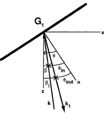
y-axis) and the outgoing wave-front and z-axis, respectively, as in Figure 3.9. We will call the incoming wave-front angles φ and β. Using these variables, the diffraction grating equation (Equation 3.2) becomes:

sin (θL±βi) =

2kLsinθL

kcosφ −sin (θL±β). (3.34) Assuming the incoming wave-front is on axis (i.e. parallel to the interferometer arm), β=φ= 0, which gives:

sin (θL±βi) =

2(kL−k) sinθL

k . (3.35)

Expanding the sine term, we calculate:

βi=±2 tanθL

k−kL

(33)

[image:33.612.214.389.88.279.2]

Figure 3.9: One diffraction grating, G1, in the SHS. The z-axis runs parallel to the interferometer arm containing G1. An incoming wave-front that is not traveling parallel to the interferometer arm is an angleβ from thez-axis. The y-axis is not shown in the figure as it is coming out of the page. Thex-axis runs perpendicular to the z andy-axes. Here,θ is the Littrow angle [8].

Because we want the interference pattern as a function ofx, we compute thex-components of the two wave-vectors from their respective gratings:

kx1 = 2πksin (±2 tanθL

k−kL

k ) kx2 = 2πksin (±2 tanθL

k−kL

k ),

(3.37)

where we have assumed that φi =φ. These components add together when they recombine

at the detector:

kx1+kx2 = 2π·4(k−kL) tanθL, (3.38)

where we see the Fizeau spatial frequency term.

(34)

OP D= 4xtan(θL). (3.39)

The spectral variable in the SHS is also different from typical FTIR instruments. Instead of our interferogram being a function of wavenumber, k, it is a function of the difference wavenumber, k−kL. The phase difference between the recombining beams in the SHS is

then:

∆φ= 2π·4(k−kL) tanθLx (3.40)

and the interferogram as a function of position,x, along the detector for a monochromatic source is given by:

I(x) = 1

2L(k)[1 + cos (2π·4(k−kL) tanθLx). (3.41) For a poly-chromatic source, the interferogram becomes:

I(x) =

Z ∞

−∞

1

2L(k)[1 + cos (2π·4(k−kL) tanθLx)]dk, (3.42) whereL(k) is the spectral radiance measured at the input andL(−k) is the same function asL(k) but flipped [8]. As in the other FTS instruments, the IFT of the interferogram gives the spectrum of the input.

3.4.3 SHS Limitations

The high resolution and throughput, lack of moving parts, and compact size of the SHS make it a very robust and versatile instrument. Yet, the SHS does have its limitations.

The resolving power of the SHS depends on the width of the diffraction grating. This, in turn, limits the observable bandpass. A larger grating is needed to view a wider bandpass region. Also, at low resolving powers, the accepted angle of light hitting the detector may be greater than the angle between the orders of diffraction, allowing undesired light, or noise, to reach the detector [25].

Because each pixel in the SHS detector sees a different interferometer path, the arms and detector must be aligned very carefully. The system must also be flat-fielded so that the gain and dark current of each pixel is taken into account during the measurement process. These restrictions also increase the computation time for the SHS system. The necessary flat-fielding and phase corrections must be done thoroughly. Signal apodization is also needed to avoid truncation errors in the spectra (see Section 5.2.4), which also reduces the resolving power [25].

(35)

NESR is achieved when the only noise source in the system is shot noise, i.e. the noise associated with the arrival of photons at a detector. This ideal NESR is known as the shot-noise-limited NESR [34].

3.4.4 Imaging SHS

Thus far, our discussion of the SHS has only been concerned with the interferometric applications of the SHS. However, the SHS can be used to collect hyperspectral imagery using additional optics [9]. An anamorphic telescope at the entrance aperture of the SHS images one dimension of the spatial scene onto the diffraction gratings while defocusing the other dimension. Depending on how your system is oriented, the anamorphic telescope looks at either a row or column of pixels at a time as in Figure 3.10. Each pixel in the row or column can be considered a point source in the scene. Each point source creates a line image across the diffraction gratings, perpendicular to the grating grooves. This results in an individual interferogram corresponding to each imaged pixel across the detector. Thus, the spatial information is recorded along one dimension of the detector array, while the spectral information is recorded in the other as in Figure 3.10. By scanning the scene by either columns or rows or pixels, we can collect an entire hyperspectral data cube.

(36)

Chapter 4

Previous LWIR Interferometry

Technologies

Spatial heterodyne spectroscopy is still a relatively new field and, therefore, other interferometers have been used to measure and exploit spectra in the past. As mentioned earlier, several SHS instruments have been created for the UV-VIS regions for astronomical purposes. However, only one SHS instrument has been successfully designed and built to operate in the LWIR [14]. This is mainly due to the high complexity and expense of LWIR-transmitting optical materials. Below, we describe some specific instruments that are similar in design, theory, or application to the instrument design used in the examples in this thesis. All the instruments discussed in this section operate in the LWIR because the results in this thesis are for a LWIR SHS design example. For a summary of the different technologies, see Appendix A.

4.1

FIRST (Field-portable Imaging Radiometric

Spectrom-eter Technology)

The Field-portable Imaging Radiometric Spectrometer (FIRST) is developed for standoff chemical detection. Developed by Telops, FIRST operates over 8 to 11.5 microns. The spectral resolution, determined by user-specified parameters, ranges from 0.25 to 150cm−1_.

(37)

Figure 4.1: FIRST by Telops is an imaging Michelson interferometer operating in the LWIR. Depicted here is the interferometer subsystem [10].

4.2

LIFTIRS (Livermore Imaging Fourier Transform Infrared

Spectrometer)

The Livermore Imaging Fourier Transform Infrared Spectrometer (LIFTIRS) is an imaging Michelson interferometer that can be used in the 3 to 5 micron or the 8 to 12 micron region. It has a variety of applications, including the ”identification and mapping of gaseous effluents, the remote measurement of surface temperatures and the remote classification of surface material types based on their emissivity in the infrared” [11]. Like FIRST, the spectral resolution is defined by the user and can be as high as 0.25 cm−1. An 128x128 hyperspectral image (HSI) with a spectral resolution of 4cm−1 _{takes about 5}

seconds to collect (as in Figure 4.2), more than twice the collection time of FIRST [11].

4.3

THI (Thermal Hyperspectral Imager)

(38)

[image:38.612.190.420.89.291.2]

Figure 4.2: The LIFTIRS collection time is approximately twice that of the FIRST collection time while using the same image size and spectral resolution [11].

4.4

AIRIS (Adaptive Infrared Imaging Spectroradiometer)

The Adaptive Infrared Imaging Spectroradiometer (AIRIS) built by Physical Sciences, Inc. (PSI) is a LWIR, imaging, low-order, tunable Fabry-Perot etalon spectrometer (Figure 4.4). AIRIS provides enough resolution to distinguish spectral emissivities of chemical vapors in the air with a spectral coverage of 8 to 11 microns. The tuning system allows for the collection of an interference pattern at each observed wavelength with an NESR of about two times the shot-noise-limited NESR. Gittins et al. [13] [35] have shown that AIRIS can detect multi-species chemical vapor plumes as well as clouds of biological stimulants, using target detection algorithms. The AIRIS system is capable of detecting toxic industrial chemicals (TICs) and chemical warfare agents (CWAs) based on known spectral features with a detection accuracy as high as 85% [36]. AIRIS captures a 128x128 image at a particular wavenumber in about 1 minute. Again, the FPI requires moving one parallel plate to collect the transmitted intensity at a variety of wavenumbers [37].

4.5

IRISHS (Infrared Imaging Spatial Heterodyne

Spectrom-eter)

(39)

[image:39.612.138.470.94.295.2]

Figure 4.3: The THI uses a Sagnac interferometer to collect HSI at a spectral resolution of about 16cm−1 [12].

Figure 4.4: The AIRIS is a tunable Fabry-Perot interferometer with built-in hot and cold blackbodies for internal calibration [13].

(40)

[image:40.612.96.518.93.355.2]

Figure 4.5: The IRISHS uses an IR SHS with a FPA to record an image of the sampled scene and an interferogram for each pixel in the image [4].

4.6

SHIMCAD (Spatial Heterodyne Imager for Chemical

and Atmospheric Detection)

The US Naval Research Laboratory’s Englert et al. [14] recorded the first broadband LWIR measurements from an SHS. Their instrument, the Spatial Heterodyne Imager for Chemical and Atmospheric Detection (SHIMCAD), uses an anamorphic telescope to image one dimension of the scene onto the interferometer aperture, an SHS to create the Fizeau fringes, and a FPA to collect the image and pixel interferograms. The telescope has a field of view (FOV) of 4 by 4.5 degrees, a 61 by 20 mm aperture size, and a wavenumber range of 1196 to 862cm−1, corresponding to a wavelength range of about 8.4 to 11.6 microns. The interferometer has a Littrow wavelength of 8.4 microns (or wavenumber of 1190cm−1_),

(41)

[image:41.612.188.421.173.409.2]

focal plane array. The first laboratory tests used methanol and Kapton®foil samples. The recorded SHIMCAD spectra show similarities to that recorded with a traditional FTIR spectrometer (with a resolution of 1cm−1). The measurements provide evidence of the feasibility of a LWIR SHS for field measurements [14].

(42)

Chapter 5

Design Objectives

As stated above, this thesis aims to promote the study and advancement of the SHS technology. In support of this effort, an SHS model is developed. Although the results in this thesis are for a particular design example in the LWIR, the model employs general SHS concepts and can be used for a variety of applications and design requirements. Similarly, the interferogram processing algorithm may be applied to other SHS instruments. The model and algorithm are developed focusing purely on the interferometry aspects of the SHS, though they can be adapted to incorporate imaging aspects as well.

5.1

SHS Modeling: Errors to Consider

The SHS model developed in this thesis will rely on the basic theory in Section 3.4.2. The general model concepts used are outlined by Cooke et. al [4]. Other factors to consider in generating realistic interferometric data are:

• A wavelength-dependent optical transmission function. • Phase errors.

• System vibrations. • Noise.

5.1.1 Optical Transmission Function

(43)

5.1.2 Phase Errors

There are two main components for the SHS system phase error. One part is independent while the other is dependent. The wavenumber-dependent phase error is usually rather complicated. Typically, this phase error is charac-terized after the instrument is built (or after the final design is known, using ray-tracing software) and accounted for in the interferogram processing algorithm or by methods outlined in [38] and [39].

The wavenumber-independent phase error is easy to determine from the data and, therefore, simple to correct. It refers to the interferogram’s center-burst shift from the zero-location on the detector. The position,x, along the detector, ranges from −xmax[cm] to

+xmax[cm]. Because the SHS interferogram is heterodyned about the Littrow wavenumber,

it should be symmetric and the location of its highest magnitude, i.e. the ”center-burst”, should occur atx= 0cm. Due to alignment errors in the instrument, this usually does not happen. A simple use of the FT shift theorem, however, can correct for this and place the center-burst at its correct location [4] as we will see in Section 5.2.2.

5.1.3 System Vibrations

System vibrations can be caused by thermal energy or movement of the instrument platform. These can be modeled as random events. Thermal and motion control capabilities can be built into the system to eliminate as much of these effects as possible. Thermal fluctuations mostly affect the spectral radiance calibration process. The SHS model has built-in hot and cold blackbodies for internal calibration, but if the blackbodies have fluctuating temperatures, this introduces an error in the calibration process. Motion within the instrument affects the interferogram sample spacing precision and the Littrow angle precision.

5.1.4 Noise

There are many different types of noise that can affect a system’s output. We can calculate a standard deviation for each noise source and add it to our measured signal in a Gaussian fashion. The most significant noise source, in many cases, is shot noise, which refers to the statistical variations in the number of photons converted to photo-electrons at the detector. We assume that the number of electrons we measure is large enough such that the shot noise has a Gaussian distribution rather than a Poisson distribution. If our measured interferogram, which contains signal contributions from the system self-emission, isI(x) with irradiance units ofW/m2, we can convert this to a number of electrons incident on the detector by:

Smeas(x) =

I(x)Adtint·QE

(44)

wheretintis the integration time,Adis the unit detector area,QE is the detector quantum

efficiency, his Planck’s constant, and cis the speed of light. Using our signal in electrons, we can calculate the Gaussian standard deviations associated with our noise sources in terms of electrons, starting with the shot noise:

σshot=

hp

Smeas(x)

i

avg. (5.2)

The next noise source we will consider is calibration noise. In Section 5.1.3 we said that temperature fluctuations in the internal blackbodies can cause calibration errors. We can capture these errors with an approximate calibration error rate,c, giving a calibration

noise standard deviation of:

σcalib=calibσshot2 . (5.3)

There is also a noise source associated with the detector and readout noise:

σdet=

2 AaΩdkD∗τtot

√

AdT

·Cavg, (5.4)

where Aa is the area of the system aperture,D∗ is the specific detectivity,τtot is the total

optical transmission function, which accounts for transmission functions, beam-splitter and grating efficiencies, etc.,T is the frame rate, and Cavg is the constant used to convert from

spectral radiance to number of electrons in the interferogram domain:

C(k) = AdΩtint·QE (hc/k)δk ·

r

N

2 , (5.5)

whereN is the number of interferogram samples and the factor of

q

N

2 gives us the noise

standard deviation in the interferogram domain rather than the spectral domain [41]. Cavg

is the mean value of C. The electronics noise is caused by components following the detector, mainly the pre-amplifier, and has a standard deviation of:

σelectronics =

4xmaxN P SD

AaΩRDτtot

√

T ·Cavg, (5.6)

where N P SD is the noise-power spectral density, sometimes called the input to the pre-amplifier, andRD is the detector responsivity. The next noise source to consider is that

associated with the bit error rate,B:

σbit =

v u u t bit M

q=M−1

X

q=0

2q_L max

2M₋₁

2

·Cavg, (5.7)

where M is the number of bits used in the system and Lmax is the maximum accepted

(45)

radiance units). Finally, we consider the quantization noise. Quantization is the process of rounding measurements values to a certain precision. The level of precision depends on the number of bits used in the system. The quantization noise has a standard deviation of:

σquant =

Lmax

√

12(2M ₋₁₎·Cavg. (5.8)

The total noise standard deviation is:

σtot =

s X

i

σ2

i. (5.9)

As mentioned in Section 3.4.3, an important figure of merit of our system is the overall noise-equivalent spectral radiance (NESR). We define the NESR as:

N ESR(k) = σtot

C(k). (5.10)

We can then use the NESR to calculate our SNR and a noise-equivalent change in temper-ature (NEdT). Our SNR is:

SN R(k) = Lrecovered(k)

N ESR(k) , (5.11)

whereLrecovered(k) is the recovered spectral radiance signal. Our NEdT is:

N EdT(k) = N ESR(k)_dL BB

dT

, (5.12)

where dLBB

dT is the derivative of the Planck equation for the spectral radiance of a blackbody

with respect to temperature,T. In this work, we assume a temperature of 300K.

Another form of noise we must consider in the SHS model is the pixel-to-pixel sensitivity variation in our detector. Each detector element has an individual dark current and overall sensitivity to incoming photons. We can account for the differences in sensitivity across our detector once it is built [42].

5.2

Interferogram Processing Concepts

The errors listed above, among others, must be accounted for in the interferogram processing algorithm. Specifically, the algorithm must perform the following tasks:

(46)

• Bias removal • Apodization

• Inverse Fourier Transform • Noise reduction

• Spectral Radiance Calibration

5.2.1 Flat-fielding

Flat-fielding describes the process of correcting sensor data for variations in the pixel-to-pixel sensitivity. These variations are constant and need only to be characterized after the instrument is built. Generally, the flat-fielding correction process corrects for sensitivity measurements in the detector as well as alignment errors in the interferometer arms. There are a number of ways to perform flat-fielding correction. Often, the flat-fielding correction is done in conjunction with the calibration process. However, the sensitivity variation in the detector can significantly affect the SNR, decreasing the overall quality of the retrieved spectra. Therefore, it is often desirable to characterize these errors in the laboratory for a built-in flat-fielding correction process, separate of the system calibration [42].

Englert and Harlander [42] outline three flat-fielding processes for SHS. The first assumes that the interferometer arms are exactly aligned, the second assumes misaligned arms, and the third assumes misaligned arms and corrects for phase shifts. We will explain the latter two, since there is always some error in the arm-to-arm alignment.

For the misaligned-arm correction, the flat-fielding process requires two measurements of the same source. One measurement is made with one interferometer arm blocked and the second measurement is made with the opposite arm blocked. Using these two measurements, we can correct future measured interferograms. First, we calculate the biased, partially corrected interferogram:

IC0(x) = I(x) Ia(x) +Ib(x)

, (5.13)

whereI(x) is any measured interferogram,Ia(x) is the interferogram of the known source

with one interferometer arm blocked, Ib(x) is the interferogram of the same source with

the opposite arm blocked, andIC0(x) has a modulated and unmodulated term as in Equa-tion 3.11. Next, we remove the unmodulated term. The flat-field corrected interferogram is then:

If f(x) =IC(x)·

IA(x) +IB(x)

2pIA(x)IB(x)

, (5.14)

(47)

The misaligned-arm and phase shift correction technique requires a monochromatic source for characterization and the ability to change the length of one of the arms. Three interferograms are recorded using the same monochromatic source, but three different interferometer arm lengths. Each interferogram has a different phase. We can determine the three phases by:

φi(k0, x) = arctan

Im[Ii,k0(x)] Re[Ii,k0(x)]

−k0x, (5.15)

wherei= 1,2,3, corresponding to each of the three measurements, andk0is the wavenumber

of the monochromatic light source. As expected, the interferograms have a modulated and unmodulated term. The modulated term is calculated by:

M(k0, x) =

Ii,k0(x)−Ij,k0(x) cosφi(k0, x)−cosφj(k0, x)

, i6=j, (5.16)

whereiandj are chosen on a pixel-by-pixel basis, such that the denominator is never zero. The unmodulated term is:

N(k0, x) =I1,k0(x)−M(k0, x) cosφ1(x). (5.17) To remove the unmodulated term, we divide our measured interferogram byN(k0, x) and

then subtract the mean. To remove the phase errors, we then divide byM(k0, x). Now, we

have a flat-fielded and phase-corrected interferogram. This phase-correction should correct both phase errors described in Section 5.1.2.

5.2.2 Phase Correction

From Section 5.1.2, we know that there are two different phase errors to be corrected in the processing algorithm. The wavenumber-dependent phase error can be characterized once the instrument is built [42, 39]. The wavenumber-independent phase error causes the shift of the interferogram center-burst from the zero path difference (ZPD) location. We can correct this by implementing the FT shift theorem.

If the center-burst is located a distance, +xc from the ZPD, then we can shift the

interferogram to be centered at ZPD by:

I(x)p =I(x)∗δ(x+xc), (5.18)

where δ(x+xc) is the dirac delta function centered at xcand∗ denotes the convolution.

By means of the Fourier transform modulation theorem, we can re-write this in terms of the FT pairs:

(48)

where the FT ofδ(x+xc) is exp (2π·xc·x).

Because the recorded interferogram is discrete, we can only shift the function by an integer number of sample spaces using the convolution method. In the more common case, when our interferogram is shifted by a non-integer number of sample spaces, Ben-David et al. [43] derive an approximation of the location ofxc by:

xc=dx

P

ii|I(xi)|

P

i|I(xi)|

−i0

, (5.20)

where i0 is the current sample index of the apparent ZPD in the recorded interferogram.

An estimate ofi0 can be found by locating the sample of the maximum of the recorded

interferogram. Using this value forxc, we can shift the interferogram by the FT method.

Even after the interferogram is shifted such that the ZPD is located at the center, the interferogram is still usually not perfectly symmetric. As stated earlier, to retrieve the sample spectrum, we must take the IFT of the interferogram. Our recorded interferogram will never have imaginary parts because we cannot make imaginary measurements. If the recorded interferogram is also symmetric, the IFT will also be real and symmetric. If the interferogram, however, is anti-symmetric, the IFT will have both real and imaginary parts and be odd. A signal with real and imaginary parts will have an additional phase, which we must also correct. We will explain this phase correction in Section 5.2.5.

5.2.3 Bias Removal

From Equation 3.11, we know the measured interferogram is a sum of a modulated and unmodulated term. The modulated term is the interferogram, by definition, whereas the unmodulated term may be neglected. We determine the interferogram bias, the unmodulated term, by averaging the samples on either side of the interferogram center-burst. Once the bias is determined, we subtract it from the measured interferogram so that we are left with only the modulated term.

5.2.4 Apodization

At this point, we have been describing the interferogram equation for a polychromatic source as an infinite integral. In reality, we cannot achieve infinite values for the xmax.

Thexmax is actually limited by the detector width and can be described by a rectangular

function:

RECT(x) =

1 if 0≤x≤xmax

0 otherwise (5.21)

where xmax is the maximum achievable position, x, along the detector within a given

(49)

axis is the scale of thexmax term. The SHS output is the infinite interferogram multiplied

by the detector widths RECT function. The interferogram data is cut off abruptly at the

[image:49.612.215.389.164.298.2]

−xmax and +xmax values. In signal processing, this is known as truncation [33].

Figure 5.1: The RECT function has unit amplitude between −xmax and xmax [15].

In the finite (realistic) case, the spectral radiance is:

Lrecovered(k) =

Z ∞

−∞

1

2 ·I(x)·RECT(x) cos (2πνFx)dk[4]. (5.22) By the modulation theorem, the Fourier transform (FT) of the product of two functions is equal to the convolution of the FT’ed factors:

F T {a·b}=F T {a} ∗F T {b}=A∗B[33]. (5.23) The finite-x spectral radiance is:

Lrecovered(k) =L(k)∗SIN C(k), (5.24)

where the SINC function is the Fourier Transform of the RECT function in Equation 5.21. The theoretical maximum resolution of an interferometer is given by the full-width half-maximum (FWHM) of the characteristic SINC function, which can be calculated by:

R= 1.207 2xmax

(5.25) and can be improved by making a larger interferometer with a greater maximum achievable xmax [21].

(50)

SIN C(k) = sinπk

πk [33]. (5.26)

Figure 5.2: The SINC function has a center peak with oscillations on either side that eventually go to zero amplitude [16].

A plot of the SINC function is shown in Figure 5.2. As is shown in the plot, the SINC function consists of one large central and many side lobes, some with amplitudes greater than 0.2. If the interferogram is truncated with the RECT function, the data points at either end of the truncated plot will not have an amplitude of zero. The IFT of the truncated interferogram will cause the SINCs many side lobes to spread the spectral energy from the lower frequencies to the higher frequencies [28].

Because leakage is due to the signal truncation, or the abrupt detector cutoff, we can reduce its effects by smoothing out the ends of the RECT function. This, in turn will decrease the number of and amplitude of the SINCs many side lobes. This is done by multiplying the discrete, finite interferogram by an apodization function that slowly decays to zero at the endpoints. There are a number of different apodization functions that are often used, depending on the application. The first column in Figure 5.3 shows some of the more well-known apodization functions. The second column shows the FTs of the apodization functions and the third column shows a magnified view of the FTs side lobes. Here, the unity function is what we have referred to as the RECT function. One can see that the amplitudes of its FTs side lobes are much greater than the other functions. The smaller-amplitude side lobes are less effective in spreading information into the wrong frequencies [33].

(51)

5.2.5 Inverse Fourier Transform

As previously mentioned, taking the IFT of the measured interferogram gives the measured spectrum. We know that the measured interferogram is real and should be symmetric. The FT of a real and symmetric function is also real and symmetric. The FT of a real and anti-symmetric function, however, has both real and imaginary parts and is odd. We know that measured spectral radiance should be a real function. Also, we said earlier that the SHS interferogram is a function ofL(k) where kcan be negative or positive andL(−k) is equal in magnitude to L(k). This means, our interferogram is the FT of the mirrored radiance spectrum. We want the IFT of the interferogram to be real and symmetric. If it is not, it will have an induced phase error we need to correct. We do this by taking the magnitude of the spectrum after the IFT:

Lrecovered(k) =

q

Lrecovered,R(k)2+Lrecovered,I(k)2, (5.27)

whereLrecovered,R(k) and Lrecovered,I(k) are the real and imaginary parts of the IFT of the

interferogram, respectively [44].

It is necessary to take the magnitude of the IFT, rather than just throw the imaginary part away because we want to maintain the spectrum power. From Parseval’s theorem [33], we know that:

Z ∞

−∞

|f(x)|2_dx₌

Z ∞

−∞

|F(k)|2_dk, _(5.28)

where |f(x)|2 _{is the power of the sample spectrum and}_|_F_(k)_|2 _{is the power spectrum of}

the sample spectrum. Simply removing the imaginary part of the IFT of our interferogram would reduce the power spectrum, reducing the power of the recovered spectrum as well. Therefore, taking the magnitude of the IFT ensures we do not lose any necessary information about our spectral signal.

Finally, we just said that the measured interferogram is actually the FT of the mirrored spectrum. We only need half the recovered information, mainly the half that is a function of +k. Therefore, we can discard the firstN/2 samples.

5.2.6 Noise Reduction

(52)

the median filter makes it slightly more appropriate for signal processing in the spectral domain because it preserves the emission and absorption lines in the spectra [28].

5.2.7 Spectral Radiance Calibration

As we have mentioned, the spectral radiance measured by the SHS is the sum of the scene spectral radiance and instrument self-emission terms. The spectrum recovered by the IFT is the measured spectral radiance, so we must remove the instrument self-emission to retrieve the true spectral radiance of the imaged scene. The measured spectral radiance includes one more term, the instrument responsivity. The responsivity is a function of wavenumber and describes how sensitive the system is to each wavenumber. Therefore, the actual measured spectral radiance is:

L(k) =r(k)[Lscene(k) +g(k)] (5.29)

and if we know the responsivity,r(k), and the system offset, g(k), we can calibrate the measured spectral radiance to the scene spectral radiance by:

Lscene(k) =

L(k)

r(k) −g(k). (5.30)

The instrument offset varies with instrument temperature and must be calculated often (usually between each measurement). We use a hot and a cold blackbody (BB) source for spectral calibration calculations. These calculations are usually performed within the instrument on a measurement-by-measurement basis using built-in hot and cold BB sources, as in AIRIS [36]. The hot BB has a temperature just above the ambient temperature, while the cold BB has a temperature of approximately ambient temperature, or just below ambient temperature. If the respective radiance measurements of the hot and cold BB’s areLH(k) andLC(k) at temperatures,TH andTC, the responsivity is:

r(k) = LH(k)−LC(k) LBB(TH, k)−LBB(TC, k)

, (5.31)

whereLBB(TH, k) and LBB(TC, k) are the expected BB radiation measurements of a hot

and cold BB at temperaturesTH and TC, respectively. The instrument offset is then:

g(k) = LC(k)

(53)

[image:53.612.134.465.106.599.2]

(54)

Chapter 6

Experimental Approach

The first objective of this research is to create a radiometric model of the SHS. The second objective is to develop a processing algorithm, with real-time capability, to convert N-point SHS interferograms into calibrated spectral radiance. The experimental approach consists of simulating realistic interferometric data with the model and then using the simulated interferograms to test the algorithm. This process is repeated until desired results are achieved. Both the model and algorithm are implemented in MATLAB.

6.1

SHS Model and Interferogram Simulation

The SHS system developed in this research is shown in Figure 6.1. The sample spectrum provides the system input. The SHS measures its interferogram which is then processed to best-recover the input spectral radiance. Post-processing on the retrieved spectral data is possible for future work, depending on the SHS application.

The general SHS Model developed in this thesis has the following blocks:

1. System Input 2. Entrance Optics 3. Interferometer 4. Exit Optics 5. Detection 6. System Output

(55)

Figure 6.1: The entire SHS system consists of the input, or the scene spectral radiance, the SHS itself, and processing software to determine the measured spectral radiance.

Figure 6.2: Cooke et. al’s model accepts the sample radiance with added background radiance. The input undergoes the entrance optics, Optics I, the SHS configuration, Interferometer, the exit optics, Optics II, and the detection scheme (Field-Stop, Filter, FPA, and Cold Shield) [4].

6.1.1 SHS Parameters

We begin with the user-defined SHS operational parameters: • minimum accepted wavenumber,kmin

• maximum accepted (Littrow) wavenumber,kL

(56)

• number of interferogram samples,N • diffraction grating order,m

• diffraction grating groove density,d

As we will soon see, the model generates a high resolution interferogram with NH number

of samples before the detection scheme. The detection scheme then resamples the signal at N samples. Using the above parameters, we calculate additional SHS parameters:

• Littrow angle of the diffraction gratings,θL, from Equation 3.26

• diffraction grating width,W, from Equation 3.27

• maximum value of positionx along the detector,xmax, from Equation 3.28

• high resolution number of samples,NH

• high spectral resolution,dkH

• high resolution sample spacing,dxH

• spectral resolution,dk, from Equation 3.29 • sample spacing,dx, from Equation 3.30

Again, we have defined spectral resolution and sample spacing parameters for both the high resolution interferogram generated by the model and the lower resolution interferogram sampled by the model’s detection scheme. We calculate dkH and dxH from:

dkH =

2·kL

NH

(6.1) and

dxH =

2·xmax

NH

, (6.2)

respectively, whereNH is:

NH = 2(kmax−kmin). (6.3)

6.1.2 Input

(57)

6.1.3 Entrance Optics

The first block is the Entrance Optics block. The Entrance Optics incorporate the instrument self-emission, FOV, and optical transmission. The FOV is a constant and we can factor it out later. As mentioned earlier, the instrument self-emission is added to the scene radiance. The self-emission term is modeled as a BB radiator with unit emissivity and temperature of 290K, calculated by the Planck equation:

LBB(k) = 2·108hc2k3

1 exp [hc_k(100k)

BT −1]

, (6.4)

where wavenumber, k, has units of cm−1, kB is Boltzmann’s constant, and T is the

temperature of the blackbody. Finally, the transmission of the Entrance Optics is assumed to be wavenumber-dependent. The output of the Entrance Optics is, therefore:

L0(kn) = Ω·τ1(k)Lscene(kn) +Lself,1(kn,290), (6.5)

where Ω is the system FOV (not the aperture FOV described earlier),τ1(k) is the

transmis-sion function of the Entrance Optics,knis the discrete variable for wavenumber,Lscene(kn)

is the input sample spectrum, andLself,1(kn,290) is the self-emission term of the entrance

optics. The system FOV is found by:

Ω = π

4(f /#)2_{+ 1}, (6.6)

wheref /# is the system F-number.

6.1.4 SHS Interferometer

The next block is the SHS Interferometer block. Here, we employ the interferogram equation, Equation 3.42. Now, however, we must account for the diffraction grating efficiencies and vibrational and phase errors. The measured radiance at the detector is now:

L00(k) = (1 2ηA+

1 2ηB)L

0_(k), _(6.7)

whereηA and ηB are the efficiencies of diffraction gratings A and B, respectively. After

accounting for the vibrational and phase errors, the Fizeau frequency becomes:

νF = 2(k−kL) tanθL+ 2(k−(kL+ke)) tan (θL+θe), (6.8)

where θe is the angle of error between the Littrow angles of the two gratings and ke is

the Littrow wavenumber associated with the diffraction grating Littrow angle, θL+θe.

(58)

I(xm) =

NH/2−1

X