Multivariate Lévy Models by Linear Combination: Estimation

(1)

City, University of London Institutional Repository

Citation

:

Ballotta, L., Loregian, A. and Fusai, G. (2015). Multivariate Lévy Models by Linear Combination: Estimation. London: SSRN.

This is the published version of the paper.

This version of the publication may differ from the final published

version.

Permanent repository link:

http://openaccess.city.ac.uk/16271/

Link to published version

:

Copyright and reuse:

City Research Online aims to make research

outputs of City, University of London available to a wider audience.

Copyright and Moral Rights remain with the author(s) and/or copyright

holders. URLs from City Research Online may be freely distributed and

linked to.

City Research Online: http://openaccess.city.ac.uk/ [email protected]

(2)

Multivariate L´evy models by linear combination: estimation

Angela Loregian1 Laura Ballotta2 Gianluca Fusai3

21st April 2015

Abstract

In this paper we propose a simple and effective two-step procedure to estimate the multivariate

L´evy model introduced by Ballotta and Bonfiglioli (2014). We assess our estimation approach via simulations, comparing the results with those obtained through a standard but more

com-putationally intensive one-step maximum likelihood estimation. The proposed method is then

applied to the computation of the intra-horizon Value at Risk for a portfolio of assets following

the model under consideration.

Keywords: Multivariate L´evy models, estimation, maximum likelihood, EM algorithm,

simulation, intra-horizon Value at Risk.

JEL Classification: C13, C15, C61, C65, G11

1 Introduction

The aim of this paper is to propose an efficient estimation procedure for multivariate L´evy processes obtained by linear transformation, as the ones introduced in Ballotta and Bonfiglioli (2014), in view of applications in portfolio risk management, like the computation of relevant risk measures such as Value at Risk and intra-horizon Value at Risk.

The interest in multidimensional asset models based on L´evy processes is motivated by the im-portance of capturing market shocks using more refined distribution assumptions compared to the standard Gaussian framework, incorporating skewness and kurtosis. From a risk management per-spective, in fact, the focus is specifically on the tails of the stock return distribution, and commonly used risk measure such as Value at Risk and intra-horizon Value at Risk aim at quantifying the economic impact of rare events. Further, for regulatory purposes these risk measures are usually obtained for short time horizons (i.e. 10 days), over which the effects of stochastic volatility are in general negligible (mainly due to the diffusive nature of the processes used for the modelling of volatility trends). In this respect, L´evy processes offer a natural and robust approach to model distribution tails compared to the Brownian motion, especially over the short period, as they allow

1_{SYMMYS - Advanced Risk and Portfolio Management; Email: [email protected]} 2

Faculty of Finance, Cass Business School, City University London, UK; Email: [email protected]

3_{Faculty of Finance, Cass Business School, City University London, UK and Dipartimento di Studi per l’Economia}

e l’Impresa, Universit`a del Piemonte Orientale “A. Avogadro”, Novara, Italy; Email: [email protected]

(3)

for extreme outcomes to happen more frequently. However, consistent and efficient estimation pro-cedures, which are essential part of the calculation of relevant risk measures, can be problematic for L´evy processes as extensively documented in Cont and Tankov (2004), for example, and references therein; these issues are exacerbated by increasing the dimension of the parameter space, which would be necessary in order to accommodate for the multivariate modelling required at portfolio level.

Linear transformations have been used extensively in the literature to build multivariate Lévy processes as these processes are invariant under such a transformation, and therefore their charac-teristic function and characcharac-teristic triplet can be obtained in a straightforward manner (see Cont and Tankov, 2004 for example). Thus, the standard approach is to model each risk driver as a linear combination of two independent processes representing respectively the systematic factor and the idiosyncratic shock, so that dependence between assets in a given portfolio is originated by the common component of the overall risk. Contributions based on linear transformations started with Vaˇs´ıˇcek (1987) for the case of Brownian motions; for the extension to Lévy processes we mention, amongst others, Ballotta and Bonfiglioli (2014) and Luciano and Semeraro (2010). In more details, Ballotta and Bonfiglioli (2014) apply the factor approach to the asset log-returns process, which allows to choose any Lévy process as factor processes, and encompasses any class of Lévy processes, from subordinated Brownian motions to jump-diffusion processes. Linear transformations have also been used in the literature to build multivariate subordinators and therefore alternative multivari-ate versions of subordinmultivari-ated Brownian motions; this is the case of Luciano and Semeraro (2010) who offer a general construction for subordinated Brownian motions, such as the Normal Inverse Gaussian (NIG) and the Carr-Geman-Madan-Yor (CGMY) processes. Extensions to a factor-based subordinated Brownian motion are proposed by Luciano et al. (2013) in order to incorporate addi-tional dependence properties. For a complete literature review, we refer to Ballotta and Bonfiglioli (2014), Luciano et al. (2013) and references therein.

A common trait to all these contributions is the presence of (either explicit or implicit) con-volution conditions, which allow to separate the dependence structure from the distribution of the margin processes. However, as argued by several authors such as Eberlein et al. (2008), this feature, although intuitive, leads to a biased view of the dependence in place as it reduces the flexi-bility of the factor model, and fails to recognize the different tail-behaviour shown by any portfolio component. In this respect, we notice that in the model of Ballotta and Bonfiglioli (2014) these convolution conditions are not necessary for the model to retain its mathematical tractability, its relative flexibility in accommodating a wide range of dependence structures, positive and negative linear correlation and a parsimonious number of parameters.

This article describes an efficient estimation procedure for the multivariate (exponential) L´evy processes model of Ballotta and Bonfiglioli (2014) with risk management applications type in view, specifically the computation of Value at Risk and intra-horizon Value at Risk for portfolios of dependent assets. Thus, we focus on the model estimation under the physical probability measure, which is in fact non-trivial as the common and the idiosyncratic factors driving the margins are not

(4)

directly observable in the market. In order to simplify this problem, although other approaches are possible, here we follow standard market practice and assume that the common factor representing systematic risk can be well-proxied by the returns on a broad-based index.

Based on these assumptions, the first contribution of this paper is a simple and effective two-step estimation procedure for the multivariate Lévy processes model of Ballotta and Bonfiglioli (2014). Step one consists in the univariate estimation of the common process parameters on the time series of index returns; the estimation of the loadings, i.e. the common factor’s weight in each margin, and the idiosyncratic components parameters is performed in Step two. To assess this estimation procedure, we also implement a standard one-step maximum likelihood approach in which all parameters of the multivariate Lévy process are estimated in a single step. The second contribution of this paper is the computation of the intra-horizon Value at Risk (VaR) for a portfolio of assets following the considered model, in this way extending the work of Bakshi and Panayotov (2010) to a multivariate setting which allows to take into account also the impact of dependence between the components of the portfolio. Traditional risk measures, as Value at Risk or Expected Shortfall, focus on possible losses at the end of a predetermined time horizon; nevertheless, investors are also interested in the exposure to loss throughout the horizon, as they often have thresholds that cannot be breached for the investment to survive. The emphasis on intra-horizon risk was first placed by Stulz (1996); Kritzman and Rich (2002) and Boudoukh et al. (2004) deal with intra-horizon risk assuming Gaussian distributed returns and considering a multi-year investment horizon, while Bakshi and Panayotov (2010) focus on the 10-day horizon relevant for regulatory purposes and consider univariate Lévy pure jump models for asset or portfolio returns. We note that intra-horizon risk measures are defined on the distribution of the minimum return; whilst under the arithmetic Brownian motion assumption this distribution is analytically known, in general it must be recovered numerically. To this purpose, we adopt the Fourier Space Time-stepping (FST) algorithm introduced by Jackson et al. (2008).

The outline of the paper is as follows. In Section 2, we review the most relevant features of the multivariate L´evy model under consideration. In Section 3 we discuss the estimation of the model, introducing a two-step estimation procedure. In Section 4 we assess the two-step estimation procedure via simulation for two particular specifications of the model (the NIG and the Merton jump diffusion process), comparing the results with those obtained via a one-step maximum likelihood estimation. Section 5 illustrates how to compute the intra-horizon Value at Risk for a portfolio of assets following the proposed model. Section 6 concludes.

2 The model

(5)

the stylized features of market quantities such as assets returns. Further, they represent a class of processes with known characteristic function via the celebrated L´evy-Khintchine representation; this feature in particular allows the development of efficient numerical schemes for the approxima-tion of potentially unknown distribuapproxima-tion funcapproxima-tions and derivatives prices based on Fourier inversion techniques.

Let us denote by Pt the price of a financial asset. In the class of exponential-L´evy models, the

pricePtis represented as

Pt=P0exp(Lt),

whereLis a L´evy process, with characteristic functionE(exp(iuLt)) =exp(tϕ(u)), whereϕdenotes

the so-called characteristic exponent. Assuming that we observe the price process on an equally-spaced time grid t= 1,2, . . . , T, the log-returns, defined as

Xt= log

Pt

Pt−1

=Lt−Lt−1,

are i.i.d. infinitely divisible random variables distributed asL1.

A convenient representation of multivariate Lévy processes can be obtained via linear trans-formation of a vector of independent Lévy processes, each representing the idiosyncratic risk, and another independent Lévy process modeling the common risk component. The construction of Ballotta and Bonfiglioli (2014) is based on this principle and is summarized in the following.

Proposition 1 Let Z, Y(j), j = 1, . . . , n be independent L´evy processes, with characteristic func-tions φZ(u;t) andφY(j)(u;t), for j= 1, . . . , n, respectively. Then, for aj ∈R, j= 1, . . . , n

Xt= (Xt(1), . . . , X

(n)

t )

0

= (Y_t(1)+a1Zt, . . . , Yt(n)+anZt)0 (1)

is a L´evy process on Rn with characteristic function

φX(u;t) =φZ 

 n X

j=1

ajuj;t 

 n Y

j=1

φ_Y(j)(u_j;t),u∈_Rn.

Further, the joint probability density function of the multivariate L´evy process Xt is

fX(x(1)t , . . . , x

(n)

t ) = Z ∞

−∞

f_Y(1)(x

(1)

t −a1z)·. . .·fY(n)(x

(n)

t −anz)fZ(z)dz. (2)

We note that as the given multivariate L´evy model admits computable characteristic function, the joint distribution is always available (at least numerically), even when the components’ distribu-tions, f_Y(1),· · ·, f_Y(n), f_Z, are not known analytically.

(6)

presence of the common factorZ, the components ofX are dependent and may jump together. In particular, for eacht≥0, the components of X(t) are positive associated if the loading factors aj

forj= 1, ..., nare all positive or negative; otherwise the components ofX(t) are negative quadrant dependent. In any case, the dependence between components is correctly described by the pairwise linear correlation coefficient

ρ_j,lX = Corr(X_t(j), X_t(l)) = q ajalVar(Z1) Var(X₁(j))

q

Var(X₁(l))

, (3)

as, for fixed aj, al6= 0,ρXj,l = 0 if and only ifZ is degenerate and the components are independent,

whilst ρ

X

j,l

= 1 if and only ifY

(j)_and_Y(l)_{are degenerate, i.e. there is no idiosyncratic factor in the}

components X(j) and X(l). Further, sign(ρX_j,l) = sign(ajal), therefore both positive and negative

correlations can be accommodated. Finally, we mention that the resulting multivariate model shows non-zero indices of tail dependence, the sign being controlled by the loading parameters. For fuller details on the characteristic triplet of the multivariate process and the dependence structure, we refer to Ballotta and Bonfiglioli (2014) and Ballotta et al. (2015).

We note the following. In first place, this construction is relatively parsimonious in terms of number of parameters involved as this grows linearly with the number of assets. Further, the adopted modeling approach is quite flexible as it can be applied to any L´evy process; Proposition 1 allows to specify any univariate L´evy process forYtandZt. In this respect, we note that differently

from Ballotta and Bonfiglioli (2014), in this work we do not impose any convolution condition on the components aimed at recovering a known distribution for the margin processes, hence allowing for a more realistic portrayal of the asset log-return features and the dependence structure in place. Finally, the model is particularly tractable as the full description of the multivariate vectorXtonly

requires information on the univariate processes Yt and Zt.

For the purpose of the testing of the estimation procedure introduced in the next sections, we select two alternative classes of L´evy processes commonly used for financial applications: a subordinated Brownian motion, represented by the NIG process, and a jump diffusion process with Gaussian severities as in Merton (1976), which we briefly review for completeness.

2.1 The Normal inverse Gaussian process (NIG).

The NIG model, introduced by Barndorff-Nielsen (1997), is a normal tempered stable process obtained by subordinating a Brownian motion by an (unbiased) independent Inverse Gaussian process. Its characteristic function reads

φX(u;t) = exp

iµt+ t

k(1−

p

1−2iuθk+u2_σ2_k₎

, u∈_R. (4)

(7)

of Xt are

c1= (µ+θ)t, c2 = σ2+θ2k

t, c3= 3θk σ2+θ2k

t, c4 = 3k σ4+ 6σ2θ2k+ 5θ4k2

t.

From the above, we observe that θ controls the sign of the skewness of Xt, σ affects the overall

variability and k controls the kurtosis of the distribution. The drift parameterµ affects the mean of the distribution, which otherwise would be concordant with the skewness, allowing to model return distributions with positive mean and negative skewness as well (and vice versa). Finally, the tails for the distribution are characterized by a power-modified exponential decay, or semi-heavy tail (see Cont and Tankov, 2004, for example).

As the density function is known in (semi-)closed form (as it is expressed in terms of the modified Bessel function of the second kind, see Cont and Tankov, 2004 for example), the parameters of the NIG model can be estimated directly using Maximum Likelihood (ML) estimation, initialized via the method of moments based on the first four theoretical cumulants derived above.

2.2 The Merton jump-diffusion process (MJD).

A L´evy jump-diffusion process has the form

Xt=µt+σWt+ Nt X

i=1

Ji, (5)

whereW is a standard Brownian motion,N is a Poisson process with rateλ >0 counting the jumps ofX, and {Ji}i∈N are i.i.d. random variables describing the jump sizes. All the random quantities

involved,W,N andJi (for alli), are assumed to be mutually independent. In the Merton’s

jump-diffusion model (Merton, 1976) jump sizes are all normally distributed, i.e. Ji ∼N(ν, τ2) for all i.

It follows that the characteristic function is

φXt(u) = exp

iuµt−u 2_σ2

2 t+λt

eiuν−τ

2_u2

2 −1

, u∈_R. (6)

The first four cumulants of Xt are

c1= (µ+λν)t, c2 = (σ2+λ(ν2+τ2))t,

c3=λν(3τ2+ν2)t, c4 =λ(3τ4+ 6τ2ν2+ν4)t.

We can observe how the parameters λ, ν and τ control the non-Gaussian part of the process; in particular,ν controls the sign of skewness (the density function is symmetric when ν = 0), whilst

λ governs the jumps frequency and therefore the level of excess kurtosis. We note that Xt has

(8)

We note that the estimation of the MJD model is far from trivial as the ML method requires a careful numerical optimization, as discussed in Honor´e (1998). Consequently, in the numerical study we implement the Expectation Maximization (EM) algorithm in the formulation proposed by Duncan et al. (2009), which has simple closed form solutions for the M-step (see Appendix A for fuller details).

3 Model estimation

For the purpose of the approach to the estimation of the given multivariate L´evy model, we dis-tinguish between whether the common factor is observable or not. The latter case is considered in Section 3.1, where we show how the computation of the sample likelihood function is possible once we integrate out the common factor. However, the maximization of the likelihood in this case turns out to be feasible only if we consider a limited number of assets in our portfolio. A second possibility would be to consider the unobservable common factor as a latent factor whose dynamic is assigned, so that the estimation procedure can be reduced to a (in general) non-Gaussian Kalman filtering problem. However, the application of these techniques is in general not straightforward and, in any case, they do not solve the dimensionality problem. A significant efficiency gain can be obtained if the latent factor is made observable by identifying it with a suitably chosen broad-based index, rather than filtering. In this case, discussed in Section 3.2, the likelihood admits a simple expression as product of univariate densities simplifying the estimation procedure.

3.1 Unobservable Common Factor: a one-step approach

In the case in which the common factor is unobservable, the joint density of the stock log-returns is given by equation (2) and therefore the likelihood function of the samplex= (x(1)_t , . . . , x(_tn))_t₌₁_...T is

L(x,θ) =

T Y

t=1

Z ∞

−∞

f_Y(1)(x

(1)

t −a1zt;θY(1))·. . .·f_Y(n)(x

(n)

t −anzt;θY(n))fZ(zt;θZ)dzt, (7)

whereθ = [θ_Y(1), . . . ,θ_Y(n),θ_Z,a] is the parameter set to be estimated.

(9)

model as discussed in Anderson and Rubin (1956).

Alternative approaches can be based on non-Gaussian Kalman filters, whose application though is not straighforward, and still exposed to the curse of dimensionality discussed above. As these filter techniques provide an estimate of the parameters and, at the same time, a way of making the latent factorZ ‘observable’, in the following we assume that the common factor is indeed observable because well proxied by a broad-based index. This would also help to solve the indeterminacy noted above, and is discussed in the next section.

3.2 Observable Common Factor: a two-steps approach

Let us assume, as it is standard market practice, that the common factor is observable through a broad-based index, such as the S&P500 index. In this case, the joint likelihood function of the common factor and stock log-returns can be written as

L(x,z;θZ, θY,a) = T Y

t=1

fZ(zt;θZ) n Y

j=1

fYj

x(_tj)−ajzt;θY(j)

. (8)

We note from the resulting log-likelihood function

lnL(x,z;θZ,θY,a) = T X

t=1

lnfZ(zt;θZ) + n X j=1 T X t=1

lnfYj

x(_tj)−ajzt;θ_Y(j)

,

that, due to its additive structure and the independence of the common factor and the idiosyncratic processes, the maximization procedure for the model estimation can be performed in two steps. The first step is represented by the maximization with respect to the parameters of the observable systematic process Z

max

θZ

lnL(z;θZ) = max

θZ T X

t=1

lnfZ(zt;θZ). (9)

The second step is given byn independent maximizations, one for each asset, of the likelihood of the idiosyncratic components with respect to the loading coefficients and the idiosyncratic processes parameters. Indeed from the very definition of our model (1), we can write each component Y(j)

as

Y(j)=X(j)−ajZ,

and therefore the likelihood functions of the idiosyncratic processes are

max

θ

Y(j),aj lnL

x(j)−ajz;θ_Y(j)

= max

θ

Y(j),aj T X

t=1

lnfYj

x(_tj)−ajzt;θ_Y(j)

, j = 1,· · ·, n. (10)

(10)

assets has the minimal additional cost of solving more independent maximization problems. As mentioned above, the second step consists ofnseparate likelihood maximization problems as in (10). An efficient way of initializing each maximization procedure is to calibrate first the loading coefficients to the sample covariance matrix in a sense to be specified below, and, conditionally on these estimates, to initialize the parameters of the idiosyncratic components via moment matching to the sample counterparties. The maximization problems (10) can then be solved iteratively by maximizing first with respect to the idiosyncratic parameters, and then, given these, again with respect to the loading parameters, until no further significant improvement in the objective functions is achieved. In practice, very few iterations are indeed required. In the estimation assessment and in the empirical application, in fact we stopped the procedure after a single iteration: we constraint the loadings to fit the covariance matrix to correctly recover the dependence structure as described below, and then the maximization of the likelihood in (10) is performed only with respect to the idiiosyncratic parameters.

As discussed in Section 2, the loadingsadetermine the dependence structure among the compo-nents of the processX; as observable information on dependence is usually limited to the covariance (or correlation) matrix of the stock returns, we initialize the vector a fitting the non diagonal en-tries of the sample covariance matrix to their theoretical counterparts predicted by the multivariate model (1). This is achieved by solving

min

a kCov(X)−ΣkF, (11)

wherek · k_F denotes the Frobenius norm,

Cov(X) =aa0Var(Z1) + diag([Var(Y(1)), . . . ,Var(Y(n))]), (12)

is the model covariance matrix and Σ denotes the sample covariance matrix (we set the diagonal entries to zero in both of them). In expression (12) we can use either the sample variance of the stock index returns or the parametric expression for the variance computed with the parameters estimates recovered through Step 1; in the first case, this step turns out to be independent of the specification of the L´evy processes involved in the multivariate model construction. For a reasonable initialization of the algorithm, we suggest to perform a simple linear regression of the stock returns on the broad-based index returns, as CovX_t(j), Zt

=aj

p

Var (Zt) for allj= 1, . . . , n(see Ballotta

and Bonfiglioli, 2014, for further details).

4 Estimation assessment

(11)

processes of the Merton jump-diffusion kind (‘all-MJD’). All required densities are generated via numerical inversion of the corresponding characteristic functions, using the Fast Fourier Transform (FFT) algorithm; alternatively the COS method suggested by Fang and Oosterlee (2008) can be adopted.

4.1 Two-step estimation procedure: a simulation study

In this section we present the results of a simulation study aimed at assessing the estimation procedure described in Section 3.2. To this purpose we consider daily log-returns of the S&P500 index and a selection of its constituents stocks; the observation period ranges from September 10, 2007 to May 20, 2013, for a total of 1434 observations per series. These data are extracted from Bloomberg database and adjusted for dividends.

The analysis is carried out as follows. We first estimate the chosen multivariate model using the index returns as proxy for Z. Then, we use the estimated parameters to generate series of the returns of the assets under consideration, to which the estimation procedure is re-applied. This allows us to recover the distribution of each parameter. We assess the estimation procedure in several cases, varying the length of the simulated series from one year up to four years of daily observations (T = [250,500,750,1000] days) and varying the number of components, considering up to 30 assets in the simulated portfolios (n = [5,10,15,30]). For each of the 16 cases taken into account we repeat the simulation and estimation S = 10,000 times, obtaining 10,000 sets of parameters, denoted by ˆθs, s= 1, . . . , S.

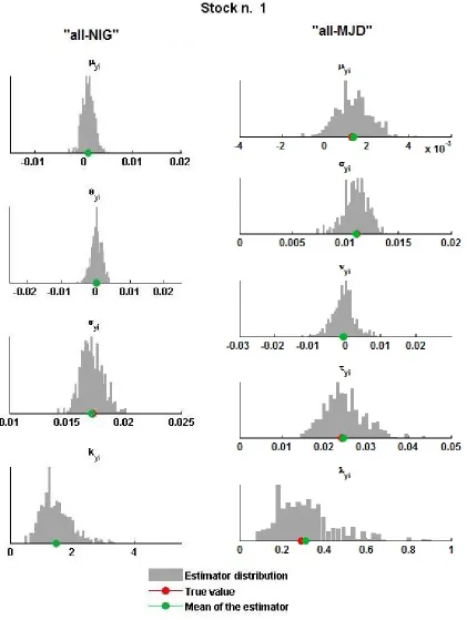
Given the large number of parameters (if n= 5 the total number of parameters is 29 for the ‘all-NIG’ model, 35 for the ‘all-MJD’ model; if n= 30 there are 154 parameters for the ‘all-NIG’ model, and 185 parameters for the ‘all-MJD’ model) we cannot display detailed results for each parameter; hence, for illustrative purpose, we show only the assessment results for the estimation of the common factorZ (Section 4.1.1), the first idiosyncratic factorY(1) and average results relative to the loadings aj, j = 1, . . . , n (Section 4.1.2). Complete results are available upon request.

The assessment is made in terms of root mean square error, bias and inefficiency, defined as

RMSE(ˆθ) = v u u t 1 S S X s=1 ˆ

θs−θ 2

, (13)

bias(ˆθ) = r

E[ˆθ]−θ2, (14)

ineff(ˆθ) = v u u t1 S S X s=1 ˆ

θs−E[ˆθ] 2

, (15)

where ˆθ indicates the estimates of the true parameter θ used in the simulation step, and E[ˆθ] =

1

S PS

s=1θˆs.

(12)

the estimation procedure of the multivariate model in the two steps presented in Section 3.2. As a positive signal in this direction, we expect the errors obtained in the assessment of the final step, which depend on the loadings estimates and indirectly on the number of components, to be comparable with those obtained in the assessment of the first step, which consists in a plain univariate estimation.

4.1.1 Step 1. Systematic component.

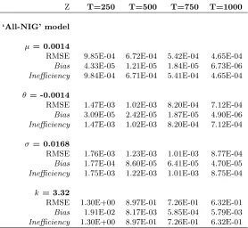
Table 1 displays root mean square error, bias and inefficiency of the estimators for the ‘all-NIG’ and ‘all-MJD’ models, as the length of the simulated series varies in T = [250,500,750,1000].

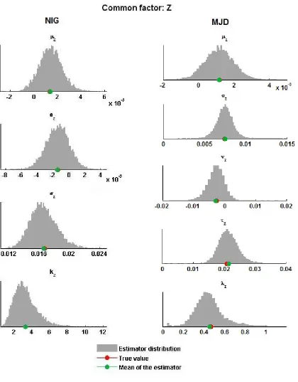
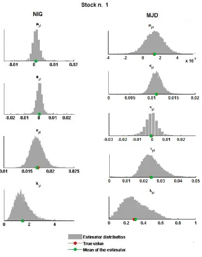
To visualize the results relative to the ‘all-NIG’ model, we plot on the left-hand side of Figure 1 the distributions of the estimators for each parameter when T = 250. The true value of the parameter, i.e. the parameter used in the simulation, and the mean of the estimator are highlighted respectively with red and green dots. The plots reveal a low level of bias for all of the estimators, and all the distributions are peaked around the mean, meaning that the maximum likelihood estimators for the NIG model are suitable for the first step of our procedure. The errors presented in Table 1 will be used as a term of comparison to evaluate the results of the final step.

The plots on the right-hand side of Figure 1 report the distributions of the estimators for the ‘all-MJD’ model parameters, highlighting the true value of the parameters in red and the mean of the distributions in green. Even in this case we observe that the estimators obtained by EM are almost unbiased and we can use the errors and inefficiency levels as benchmarks to evaluate Step 2.

4.1.2 Step 2. Loadings Calibration and Idiosyncratic Component Estimation

We implement Step 2 described in Section 3.2 by solving first the minimization problem (11) with respect to the loadings a; secondly, we use the estimated loadings to solve the n maximization problems (10) with respect to θ_Y(j) for all j = 1, . . . , n. The minimization procedure (11) is

performed by fixing the variance of the common factor equal to the sample variance of the simulated series of the processZ; in this way the assessment of this step turns out to be independent of the model specification.

(13)

Z T=250 T=500 T=750 T=1000

‘All-NIG’ model

µ = 0.0014

RMSE 9.85E-04 6.72E-04 5.42E-04 4.65E-04 Bias 4.33E-05 1.21E-05 1.84E-05 6.73E-06 Inefficiency 9.84E-04 6.71E-04 5.41E-04 4.65E-04

θ = -0.0014

σ = 0.0168

k = 3.32

RMSE 1.30E+00 8.97E-01 7.26E-01 6.32E-01 Bias 1.91E-02 8.17E-03 5.85E-04 5.79E-03 Inefficiency 1.30E+00 8.97E-01 7.26E-01 6.32E-01

‘All-MJD’ model

µ = 0.0012

σ= 0.0075

ν = -0.0025

τ = 0.0210

λ=0.47

[image:13.612.169.447.96.352.2] [image:13.612.170.446.392.648.2]

Table 1

(14)

[image:14.612.95.515.98.635.2]

Figure 1

(15)

n=5 n=10 n=15 n=30

T=250 RMSE 6.05E-02 5.23E-02 5.28E-02 6.05E-02 Bias 1.83E-03 1.65E-03 1.64E-03 1.90E-03 Inefficiency 6.05E-02 5.23E-02 5.28E-02 6.05E-02

[image:15.612.160.454.71.259.2]

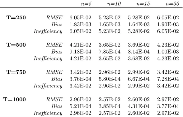
Table 2

Two-step procedure assessment: average results relative to the loading parameters a. Estimation errors expressed in absolute terms. RMSE, Bias, Inefficiency: indices computed according to equations (13)-(15).

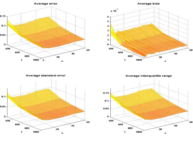
the loadings, repeating the simulation-estimation procedure 10,000 times. We then compute the average error, average bias, average standard error and average interquartile range of the loadings in correspondence of eachn, meaning that, givenn, we compute these measures for allaj, j = 1, . . . , n,

and then we take the average. The computations are repeated for simulated series of increasing length: T = [250,500,750,1000]. Results are plotted in Figure 2. The estimates of the loadings appear to be consistent, as all the average error measures decrease when estimation is performed on longer time series.

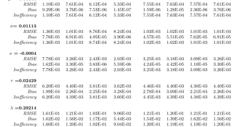
The results of the estimation of the idiosyncratic process are presented in Table 3 and Figure 3, for the case of the first asset. Results relative to the other assets are available upon request. In particular, the left-hand side of Table 3 displays root mean square error, bias and inefficiency of the estimators when the total number of assets is fixed (n= 30) and the length of the simulated series varies inT = [250,500,750,1000]. On the right-hand side of the same table, we show the assessment results for a fixed T = 500, varying the number of assets. Although the estimation of each Y(j),

j = 1. . . , n, is performed in a univariate way, the number of assets plays in principle a key role in the calibration of the loadings, which affects the estimation of the Y(j) parameters. However, consistently with the results shown in Section 4.1.2, Table 3 reveals almost uniform estimation errors forn= [5,10,15,30], showing that the number of assets has only a minimal impact on the estimation errors of the idiosyncratic terms for both the specifications we tested.

As noted above, in this section we only discussed results relative to the first asset; similar conclusions hold for all assets considered. An overview of the average performance (for the cases

n= 5 and n= 15) is provided in Table 5, discussed in more details in Section 4.3.

(16)

n=30 T=500

Y1 T=250 T=500 T=750 T=1000 n=5 n=10 n=15 n=30

‘All-NIG’ model

µ= 9.92E-04

RMSE 2.17E-03 1.13E-03 9.00E-04 7.69E-04 1.13E-03 1.12E-03 1.14E-03 1.13E-03 Bias 1.09E-05 2.80E-06 2.58E-05 4.71E-06 5.71E-06 1.19E-07 1.18E-05 2.80E-06 Inefficiency 2.17E-03 1.13E-03 9.00E-04 7.69E-04 1.13E-03 1.12E-03 1.14E-03 1.13E-03

θ = 2.15E-04

σ = 0.0173

k = 1.483

‘All-MJD’ model

µ= 0.00133

σ= 0.01113

ν = -0.0004

τ =0.02429

λ=0.29214

[image:16.612.84.548.397.652.2]

Table 3

(17)

[image:17.612.146.474.81.321.2]

Figure 2

Two-step procedure assessment: loadings. Average error, bias, standard error and interquartile range of the loadings estimates for increasing number of assets (n = 3, . . . ,60) and increasing number of observations (T = [250,500,750,1000]).

value (indicated by a red dot), revealing very little bias, and the distributions are peaked around the mean, implying that our estimation procedure performs as expected. Moreover, we observe estimation errors and inefficiency levels in line with those obtained in Step 1, therefore splitting the estimation procedure in two steps, ease of implementation aside, proves to be effective1.

4.2 One-step maximum likelihood: a simulation study

In this section we present part of the results of a simulation study relative to the estimation of the ‘all-NIG’ and ‘all-MJD’ models parameters using the one-step ML approach discussed in Section 3.1, which represent a useful term of comparison to evaluate the results obtained from the two-step procedure presented above. Hence, we use the same dataset as in Section 4.1, but we relax the assumption that the systematic risk factorZ is observable through the index.

The maximum likelihood estimation consists in maximizing the likelihood function (7); the quadrature of the integral in (7) is performed via the trapezoidal rule.

Due to the computational cost of the procedure, here we consider a small number of assets (n = 5, i.e. 24 parameters to be estimated for the ‘all-NIG’ model, 35 for the ‘all-MJD’ model) repeating the simulation 1000 times; we then perform 100 simulations to evaluate the estimation forn= 15 assets (i.e. 79 parameters for the ‘all-NIG’ model, 95 for the ‘all-MJD’ model). Results

1

(18)

[image:18.612.90.506.93.622.2]

Figure 3

(19)

relative to the common factorZ, the first idiosyncratic componentY(1) and the first loadinga1, are

displayed in Table 4. Complete results are available upon request. The estimators distributions for

(20)

n=5 n=15 n=5 n=15 n=5 n=15 (1000 sim) (100 sim) (1000 sim) (100 sim) (1000 sim) (100 sim) ‘All-NIG’ model

Z Y1 First Loading

µ= 0.0014 µ= 9.92E-04 a1= 0.8898

RMSE 7.07E-04 5.67E-04 1.19E-03 1.11E-03 4.72E-02 3.85E-02

Bias 5.82E-05 4.18E-05 2.51E-05 1.58E-04 2.36E-04 1.64E-03

Inefficiency 7.04E-04 5.65E-04 1.19E-03 1.10E-03 4.72E-02 3.85E-02

θ= -0.0014 θ= 2.15E-04

RMSE 1.11E-03 8.64E-04 1.47E-03 1.52E-03

Bias 9.64E-05 5.63E-05 1.61E-05 1.43E-04

Inefficiency 1.10E-03 8.62E-04 1.47E-03 1.52E-03

σ= 0.0168 σ= 0.0173

RMSE 1.24E-03 1.25E-03 9.95E-04 1.12E-03

Bias 3.60E-05 7.30E-05 1.04E-04 1.97E-04

k= 3.32 k= 1.483

RMSE 1.15E+00 8.35E-01 4.87E-01 4.59E-01

Bias 8.90E-02 1.29E-01 1.22E-02 4.56E-02

Inefficiency 1.14E+00 8.25E-01 4.87E-01 4.57E-01

‘All-MJD’ model

Z Y1 First Loading

µ= 0.0012 µ= 0.00133 a1= 0.8898

RMSE 6.24E-04 6.23E-04 7.85E-04 7.68E-04 5.44E-02 3.98E-02

Bias 9.65E-05 1.06E-04 4.54E-05 6.12E-05 1.08E-02 4.52E-03

Inefficiency 6.16E-04 6.13E-04 7.84E-04 7.65E-04 5.33E-02 3.95E-02

σ= 0.0075 σ= 0.01113

RMSE 1.14E-03 6.80E-04 1.12E-03 9.61E-04

Bias 3.37E-04 2.37E-04 1.02E-04 5.35E-05

ν = -0.0025 ν = -0.0004

RMSE 1.69E-03 1.85E-03 3.03E-03 3.19E-03

Bias 8.17E-05 2.73E-04 9.54E-05 7.16E-05

τ= 0.0210 τ =0.02429

RMSE 2.72E-03 3.26E-03 4.60E-03 4.27E-03

Bias 7.84E-04 1.67E-03 3.11E-04 8.71E-04

λ=0.47 λ=0.29214

RMSE 2.33E-01 1.49E-01 1.36E-01 1.15E-01

Bias 1.63E-01 8.84E-02 2.15E-02 1.20E-02

[image:20.612.133.659.65.531.2]

Table 4

One-step approach assessment. Estimation errors expressed in absolute terms. RMSE, Bias, Inefficiency: indices computed according to equations

(21)

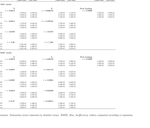
Bearing in mind the different number of simulations performed2, we can compare the results of the two-step procedure assessment with those presented in this section. In particular, for both the ‘all-NIG’ and ‘all-MJD’ models, the results relative to the common factorZ can be compared to those displayed in the second column of Table 1, corresponding to estimates based on T = 500 observations, while the results relative to the first idiosyncratic factor can be compared with those in the fifth and seventh columns of Table 3; the errors relative to the first loading estimates can be compared to those reported in Table 2, forT = 500,n= 5,15. In particular, we note that in the case of the ‘all-NIG’ model the errors obtained with the two-step procedure, using ML estimation, are in line with those obtained with the one-step ML approach, which in principle, aside computational issues, should be the preferred method, exploiting all at once the whole information contained in the data. On the other hand, in the case of the ‘all-MJD’ model, we observe instead that the errors of the two-step procedure, where the univariate estimations are performed via the less efficient EM algorithm, are just slightly larger than those obtained with the one-step ML approach.

4.3 Two-step vs one-step approach: efficiency gain index and likelihood com-parison

In order to compare the efficiency of the two approaches, both in terms of estimation errors and computational time, we modify the efficiency gain index used in Monte Carlo simulation analysis and defined for example in Glasserman (2004). Given a specification of the model (1), characterized by K parameters, we compute the efficiency gain, E21, of the two-step procedure to the one-step

maximum likelihood approach as

E21=

MSE1t1

MSE2t2

, (16)

where MSE_{1 (2)} denotes the average mean square error

MSE = PK

i=1MSE(ˆθi)

K ,

of the parameters estimated by the one-step (1) and the two-step (2) approach respectively. MSE(ˆθi)

is the mean square error (i.e. the square of the RMSE defined in equation 13) and t_{1 (2)} is the average time needed to estimate the model parameters using the 1 (2) approach. In particular, we compute the efficiency gain index in correspondence of the ‘all-NIG’ and ‘all-MJD’ models with 5 and 15 components. In the n = 5 case, for each of the two approaches, we consider the mean square errors based on 1000 simulations; forn= 15 we rely on 100 simulations.

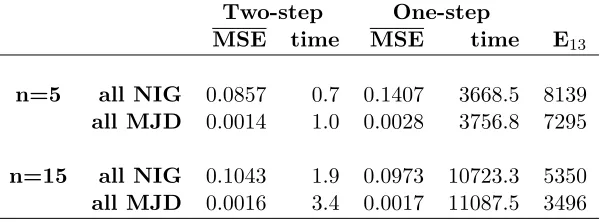
Results are reported in Table 5: we observe that the two-step approach is significantly more efficient in terms of computational time. Moreover, for n = 5 the average mean square errors attained with the two-step approach are lower than those given by the one-step maximum likelihood (8.5% vs 14% for the ‘all-NIG’ model, 0.14% vs 0.28% for the ‘all-MJD’ model), whilst they are

2

(22)

[image:22.612.100.515.105.615.2]

Figure 4

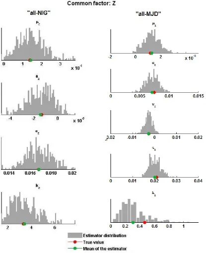
One-step approach assessment. Distributions of the estimators for the parameters of the common factor Z

(23)

[image:23.612.97.518.85.644.2]

Figure 5

(24)

Two-step One-step

MSE time MSE time E13

n=5 all NIG 0.0857 0.7 0.1407 3668.5 8139

all MJD 0.0014 1.0 0.0028 3756.8 7295

[image:24.612.157.457.72.183.2]

n=15 all NIG 0.1043 1.9 0.0973 10723.3 5350 all MJD 0.0016 3.4 0.0017 11087.5 3496 Table 5

Average MSE, computation times (measured in seconds) and efficiency gains of the two-step approach to the one step maximum likelihood. (Processor: Intel(R) Core(TM) i5-2400 CPU @ 3.10GHz 3.10 GHz; RAM: 4.00 GB)

almost the same for n = 15 (about 10% for the all-NIG’ model, 0.16% for ‘all-MJD’). According to efficiency index (16), in our experiment the two-step procedure performed 3496 times more efficiently than the one step approach in the worst case (‘all-MJD’, n= 15) and 8139 times more efficiently in the best one (‘all-NIG’,n= 5).

For a further comparison, we simulate 1,000 samples, each made of 500 observations from the ‘all-NIG’ and the ‘all-MJD’ model with 5 components, and we estimate the parameters with both methods. For each simulated sample we then compare the maximum log-likelihood achieved using both approaches; results are presented in Figures 6 and 7 for the ‘all-NIG’ model and the ‘all-MJD’ model respectively. In the top panels of both figures we report the maximum log-likelihood and the log-likelihood achieved by the two-step procedure for each simulation, sorting the simulations by increasing values of the maximum likelihood for better clarity; in the bottom panels we display the histograms of the two log-likelihood distributions. From Figure 6 we note that in the ‘all-NIG’ case, in every simulation, the estimates obtained by means of the two-step procedure lead to a likelihood which is very close to the maximum one. Conversely, Figure 7 shows that for the ‘all-MJD’ case the likelihoods resulting from the two-step routine, where the univariate estimations are performed by EM algorithm, are less close to the maximum ones.

5 Application: intra-horizon VaR

In this section we present an application relative to the computation of the intra-horizon Value at Risk for a portfolio of assets with returns following the multivariate L´evy model (1). While traditional risk measures, as Value at Risk or Expected Shortfall, focus only on losses at the end of a predetermined time horizon, intra-horizon risk measures take into account the exposure to losses throughout the investment’s life. The magnitude of losses that can occur before the end of the horizon is of paramount importance, for example, for monitored asset managers, leveraged investors, borrowers required to maintain particular level of reserves as a condition of a loan agreement or securities lenders required to deposit collateral.

(25)

[image:25.612.120.494.97.338.2] [image:25.612.110.493.100.666.2]

Figure 6

Likelihood comparison (‘all-NIG’ model)

Figure 7

[image:25.612.117.494.391.658.2]

(26)

fort ∈[0, T], be the real-valued random process describing possible paths of an asset or portfolio log-return, with initial value X0 = 0. For practical implementation, let us assume the process is

observed on an equally spaced time grid 0,∆,· · ·, M∆ =T, and define the process of the minimum

mM up to the M-th monitoring date as mM := minj=0,···,MXj∆. The VaR-I at confidence level

(1−α) is defined as the absolute value of theα-quantile of the distribution of the random variable

mM

P(mM ≤ −VaR-I|X0=x) =α. (17)

The idea is that during the investment life the path of returns can reach high negative values, which investors may care about. In such cases, the left tail of the minimum return distribution better represents risk than the left tail of the return distribution itself.

While under the arithmetic Brownian motion assumption the distribution of the minimum return is analytically known (see Kritzman and Rich, 2002 for the case with continuous monitoring, and Fusai et al., 2006 instead for the discrete monitoring one), under more general assumptions for the driving process it must be recovered numerically. To this purpose, we resort to the Fourier Space Time-stepping (FST) algorithm introduced by Jackson et al. (2008) for option pricing purposes. Our problem is indeed equivalent to finding the value of a down-and-out binary option, that is an option paying 1 if the underlying does not hit a certain lower barrier within a given time period, and zero otherwise. However, due to the nature of the application under consideration, our computations are performed under the physical probability measure.

Fixed an arbitrary thresholdy, the FST algorithm allows us to recover the value function

v(0, x) :=E[1{mM>y}|X0 =x] =P(mM > y|X0 =x)

via backward recursion, so that

vM(x) := v(T, x) = 1{x>y}

vm−1(x) = F F T−1[F F T[vm(x)]eϕ∆]1{x>y}, m= 1,· · ·, M, (18)

where ϕ is the L´evy exponent of Xt. For further details on the FST algorithm, refer to Jackson

et al. (2008).

When Xt is the return of a portfolio of assets with weights wj following the multivariate L´evy

model (1) and the time horizon is short, as in the case of the application considered here, the expression of the characteristic function of Xt, required for implementation of the FST step (18),

(27)

the asset log-returns, and exploiting the independence of Y(j),j = 1, . . . , n andZ, so that

E[exp (iγX)] = E

 exp  iγ   n X j=1

wjY(j)+Z n X

j=1

wjaj       =   n Y j=1

φ_Y(j)(γw_j)



φ_Z 

γ n X

j=1

wjaj 

 ∀γ ∈R, (19)

where we omitted time subscripts to simplify the notation3. The characteristic functions in equation (19) are then chosen according to the specified model.

Further, in virtue of the translation invariance property of L´evy processes, it follows that

v(0, x) =P(mM >(y−x)|X0= 0). Hence, the computation of the (1−α)-VaR-I can be summarized

in the following steps.

Step 1. Choose an arbitrary thresholdy.

Step 2. Compute the functionv(0, x) by means of the FST algorithm. Step 3. Find the valuex such that v(0, x) = 1−α.

Step 4. Compute the VaR-I as VaR-I=−(y−x).

[image:27.612.149.467.99.184.2]

As an application, we compute the 10 days 99% intra-horizon VaR for an equally weighted portfolio, under the ‘all-NIG’, ‘all-MJD’ and ‘all-Gaussian’ (henceforth Gaussian) models. We include in the portfolio 20 of the most capitalized stocks in the S&P500 index4. The estimation is performed on daily log-returns, from May 24, 2011 to May 20, 2013, applying the two-step procedure presented in Section 3.2. Estimates and confidence intervals at 95% level for the ‘all-NIG’ and ‘all-MJD’ models parameters are displayed respectively in Tables 7 and 8.

Figure 8 compares the sample covariance matrix with the covariance matrix estimated according to the ‘all-NIG’ model, using two color-coded matrices in which each entry is colored according to its value, and the conversion color-value is provided in the lateral color bar. We notice that the multivariate NIG model accurately reproduces the sample covariance among the assets in our dataset. Similar results are obtained for the multivariate MJD model and are available upon request5.

In order to test the ability of the fitted ‘all-NIG’, ‘all-MJD’ and Gaussian models to describe the distribution of portfolio returns, we perform a comparison with their sample distribution, as in Eberlein and Madan (2009) and Luciano et al. (2013) for example. Thus, we consider 1,000 randomly generated long-only portfolios and 1,000 randomly generated long-short portfolios.

Long-3

If returns are very volatile or the horizon is longer, it becomes essential to work with linear returns. In this case (19) no longer holds. For more details, see Meucci (2005).

4

Apple, Exxon Mobil Corporation, Wal-Mart Stores, Microsoft Corporation,Google, General Electric, IBM, Chevron Corporation, Berkshire Hathaway, AT&T, Procter & Gamble, Pfizer, Johnson & Johnson, Wells Fargo & Co., Coca-Cola, JPMorgan Chase & Co., Oracle, Merck & Co., Verizon Communications, Amazon.com.

5_{We note that under other specifications of the multivariate model only the diagonal entries change, due to the}

(28)

[image:28.612.143.470.71.238.2]

Figure 8

Sample and estimated covariance matrices for the 20 assets in our portfolio (‘all NIG’ model). The conversion color-values is provided in the side color bar.

only weights are generated by drawing an i.i.d. sample from a standard normal distribution, taking the absolute value and rescaling by the sum. Long-short portfolio weights are generated similarly, drawing an i.i.d. sample from a standard normal distribution and rescaling it by the sum of the squares. We perform the Kolmogorov-Smirnov test, deriving the probability density function by inverting via FFT the portfolio characteristic function (19). The results are displayed in Figure 9, which illustrates the empirical complementary distribution functions of the p-values across the 1,000 portfolios, namely, for each value p ∈ [0,1] we display the proportion of portfolios with p-value greater than p. The higher this proportion, the better is the model ability to capture the distribution of the return of the randomly generated portfolios. We note that both L´evy-based models significantly outperform the Gaussian one, for which the p-value is systematically smaller. Further, the ‘all-NIG’ model better fits the sample distribution of returns with respect to the ‘all-MJD’ specification for both long only and long-short portfolios.

(29)

[image:29.612.140.471.74.235.2]

Figure 9

Portfolios fit. P-values complementary distribution functions for the Kolmogorv-Smirnov test.

VaR VaR-I

Estimate CI(lb) CI(ub) Multiples Estimate CI(lb) CI(ub) Multiples

Gaussian 0.0700 0.0570 0.0833 1.0000 0.0739 0.0613 0.0867 1.0000

‘all-MJD’ 0.0736 0.0589 0.0889 1.0514 0.0784 0.0638 0.0948 1.0609

‘all-NIG’ 0.0778 0.0605 0.0966 1.1114 0.0834 0.0653 0.1022 1.1285

Table 6

10 days horizon 99% VaR and VaR-I of an equally weighted portfolio under the ‘all-NIG’, ‘all-MJD’ and Gaussian models, with confidence intervals at 95% level. Confidence intervals computed using bootstrap resampling methods, as illustrated in Appendix B.

the Brownian motion, as discussed in Section 2.

6 Conclusions

We propose an estimation procedure for multivariate asset models based on linear transformation of L´evy processes as in Ballotta and Bonfiglioli (2014), allowing to extend the use of multivariate L´evy models for risk and portfolio management applications.

[image:29.612.73.544.284.348.2]

(30)

[image:30.612.141.464.236.511.2]

Figure 10

(31)

this assumption can be relaxed as to allow any L´evy process for the idiosyncratic part across all the names included in the portfolio in order to accommodate different tail behaviours.

As an application, we employ the proposed estimation procedure for the calculation of the intra-horizon Value at Risk of a portfolio of assets following the model under consideration by means of the FST algorithm. The numerical study reveals the importance of properly capturing realistic features of asset log-returns, such as skewness and excess kurtosis, by incorporating jumps in the risk dynamic. Results from the empirical study, in fact, highlight the more conservative risk estimates offered by the intra-horizon VaR especially for the case of the NIG, reflecting the different decay behaviour of the distribution tails. Further applications to portfolio optimization problems are considered in Loregian (2013).

Extensions to several common factors can also be considered by adopting the Independent Component Analysis (ICA) approach along the lines considered, for example, in Ghalanos et al. (2015). This is left to future research.

A

EM algorithm for Merton’s JD model

To fit the Merton’s jump-diffusion model (5) we implemented the EM algorithm in the formulation proposed by Duncan et al. (2009). We report here the main ideas and the formulas needed to implement the procedure, while referring to the original work for further details. Note that, in order to simplify the solution of the EM algorithm, we follow Duncan et al. (2009) and adopt an alternative parametrization of the Merton’s jump-diffusion model (5). Specifically, we setν =ασ

and τ = βσ (with β > 0). Further, we denote by Dt the first two terms in (5) representing the

diffusion component. Then the independent random vectors

Ct=  



(Dt, Nt) (Nt= 0)

(Dt, Nt, Jt,1, . . . , Jt,Nt) (Nt>0)

t= 1. . . , T

completely determine the jump diffusion process Xt in (5). In the EM terminology, Ct are the complete data, while Xt are the incomplete data. The complete log-likelihood of C1, . . . , CT is

given by

ln(Lc(θ)) =−

1 2Tln(σ

2₎₋ 1

2σ2

T X

t=1

(Dt−µ)2−Tln(

√

2π)

− 1

2ln(τ

2₎

T X

t=1

Nt−

1 2τ2

T X t=1 Nt X k=1

(Jt,k−ν)2−ln(

√

2π)

T X

t=1

Nt

−T λ+ ln λ

T X t=1 Nt ! − T X t=1

ln(Nt!),

where θ = (µ, σ2, ν, τ2, λ) is the vector of parameters and we interpret PNt

k=1(Jt,k −ν)2 = 0 if

(32)

predictor of ln(Lc(θ)), i.e. its conditional expectation, where we condition on the available data X. The M-step gives a new estimate θ(1), which maximizes the conditional expectation computed in the E-step. Under certain general conditions, the sequence of estimates obtained in this way yields monotonically increasing values of the likelihood and converges to the ML estimator for the incomplete dataX1, . . . , XT.

The algorithm proposed by Duncan et al. (2009) is particularly efficient due to simple closed form solutions for the M-step: the optimal values ofµ,σ2,ν,τ2 and λare

ˆ

µ= 1

T

T X

t=1

Eθ0(Dt|Xt), σˆ2 =

1

T

T X

t=1

Eθ0

(Dt−µˆ)2Xt ,

ˆ

ν= 1

Tλˆ

T X

t=1

Eθ0(NtJt,k|Xt), τˆ2 =

1

Tλˆ

T X

t=1

Eθ0

Nt(Jt,k−νˆ)2|Xt ,

(20)

where

ˆ

λ= 1

T

T X

t=1

Eθ0(Nt|Xt). (21)

The formulas are made operational by evaluating the conditional expectations. First, ˆλin (21) and the two functions

at(β) =Eθ0

1 1 +Ntβ2

Xt

, bt(β) =V arθ0

1 1 +Ntβ2

Xt

must be evaluated inβ0 =σ0/τ0, knowing the conditional probability

Pθ0(Nt=k|Xt) =

ϕ(Xt;µ0+kν0, σ02+kτ02)

P∞

k=0ϕ(Xt;µ0+kν0, σ02+kτ02)

k= 0,1, . . .

where ϕ is the normal probability density function. The estimates for µ and σ2 in (20) can then be computed using

Eθ0(Dt|Xt) = µ0−

ν0

β₀2 +at(β0)

Xt−µ0+

ν0

β₀2

,

Eθ0

(Dt−µˆ)2|Xt = (Eθ0(Dt|Xt)−µˆ)

2₊_σ2

0(1−at(β0)) +bt(β0)

Xt−µ0+

ν0

β₀2

2

(33)

To find the estimates forν andτ2 in (20) the following quantities are needed:

ct(β0) = β02at(β0)(1−at(β0))−β02bt(β0)−

(1−at(β0))2

Eθ0(Nt|Xt)

,

Eθ0(NtJt,k|Xt) = (1−at(β0))

Xt−µ0+

ν0

β2 0

,

Eθ0

Nt(Jt,k−νˆ)2|Xt = τ02(Eθ0(Nt|Xt))−1 +at(β0)) +ct(β0)

Xt−µ0+

ν0

β₀2

2

+Eθ0(Nt|Xt)

ˆ

ν−Eθ0(NtJt,k|Xt)

Eθ0(Nt|Xt)

2

.

To initialize the algorithm, Duncan et al. (2009) suggest to fix the value of ν0 = 0, assuming

symmetric returns, and ofλ0= 0.2 or smaller, and then recoverµ0,β0andσ02exploiting respectively

the moment conditions

E(Xt) =µ, β2 = r

ˆ

γ

3λ 1−λ

r ˆ

γ

3λ

!−1

,Var(Xt) =σ2(1 +β2λ),

where ˆγ is the sample excess kurtosis ofXt.

B

Confidence intervals using bootstrap

The bootstrap method, introduced in Efron (1979), is used to compute the confidence intervals for the multivariate L´evy model parameters (Tables 7 and 8) and for the risk measures in Table 6. To preserve the cross sectional dependence in each bootstrap sample, we consider (xt, zt) as a single

observation: the bootstrap samples are built by drawing, out of the given sample of sizeT,T dates with replacement each time. Once obtained the distribution of the statistic of interest, we compute the confidence interval at level α as (QS(α/2);QS(1−α/2)), where the lower and upper bounds

are respectively the α/2 and 1−α/2 quantiles of the sampling distribution of the statistic S.

References

Anderson, T.W., Rubin, H., 1956. Statistical inference in factor analysis.

Bakshi, G., Panayotov, G., 2010. First-passage probability, jump models, and intra-horizon risk. Journal of Financial Economics 95, 20–40.

Ballotta, L., Bonfiglioli, E., 2014. Multivariate asset models using L´evy processes and applications. The European Journal of Finance Forthcoming.

(34)

Barndorff-Nielsen, O.E., 1997. Normal inverse Gaussian distributions and stochastic volatility modelling. Scandinavian Journal of statistics 24, 1–13.

Boudoukh, J., Richardson, M., Stanton, R., Whitelaw, R., 2004. Maxvar: Long horizon value at risk in a mark-to-market environment. Journal of Investment Management 2, 1–6.

Cont, R., Tankov, P., 2004. Financial Modelling with Jump Processes. Chapman and Hall/CRC. 2nd edition.

Duncan, J., Randal, J., Thomson, P., 2009. Fitting jump diffusion processes using the EM algo-rithm, in: Contributed talk at the Australasian Meeting of the Econometric Society, Canberra, Australia.

Eberlein, E., Frey, R., von Hammerstein, E.A., 2008. Advanced credit portfolio modeling and CDO pricing, in: Mathematics: Key Technology for the Future. Springer.

Eberlein, E., Madan, D., 2009. On correlating L´evy processes. Robert H. Smith School Research Paper No. RHS , 06–118.

Efron, B., 1979. Bootstrap methods: another look at the jackknife. The Annals of Statistics , 1–26.

Fang, F., Oosterlee, C.W., 2008. A novel pricing method for European options based on Fourier-Cosine series expansions. SIAM Journal on Scientific Computing .

Fusai, G., Abrahams, I., Sgarra, C., 2006. An exact analytical solution for discrete barrier options. Finance and Stochastics 10, 1–26.

Ghalanos, A., Rossi, E., Urga, G., 2015. Independent Factor Autoregressive Conditional Density Model. Econometric Reviews 34, 594–616.

Glasserman, P., 2004. Monte Carlo Methods in Financial Engineering. Springer.

Honor´e, P., 1998. Pitfalls in estimating jump-diffusion models. Available at SSRN 61998 .

Jackson, K., Jaimungal, S., Surkov, V., 2008. Fourier space time-stepping for option pricing with L´evy models. Journal of Computational Finance 12, 1–29.

Kritzman, M., Rich, D., 2002. The mismeasurement of risk. Financial Analysts Journal , 91–99.

Loregian, A., 2013. Multivariate L´evy models: estimation and asset allocation. Ph.D. thesis. Universit`a degli Studi di Milano-Bicocca.

Luciano, E., Marena, M., Semeraro, P., 2013. Dependence calibration and portfolio fit with factor-based time changes. Carlo Alberto Notebooks .

(35)

Merton, R.C., 1976. Option pricing when underlying stocks are discontinuous. Journal of Financial Economics 3, 125–144.

Meucci, A., 2005. Risk and Asset Allocation. Springer.

Stulz, R.M., 1996. Rethinking risk management. Journal of Applied Corporate Finance 9, 8–25.

(36)

Par. Estimate CI (lb) CI (ub) Par. Estimate CI (lb) CI (ub) Par. Estimate CI (lb) CI (ub) Par. Estimate CI (lb) CI (ub)

µZ 1.24E-03 3.11E-04 2.38E-03

θZ -7.69E-04 -2.23E-03 4.81E-04

σZ 1.19E-02 1.05E-02 1.33E-02

kZ 2.32 1.24 3.73

aY1 0.78 0.67 0.88 aY2 0.92 0.86 0.98 aY3 0.45 0.37 0.52 aY4 0.87 0.81 0.94

µY1 1.88E-04 -2.89E-03 3.09E-03 µY2 1.14E-03 -1.13E-04 3.37E-03 µY3 8.35E-04 -5.49E-04 2.77E-03 µY4 -1.87E-03 -4.63E-03 -2.94E-04

θY1 5.21E-05 -3.05E-03 3.75E-03 θY2 -1.20E-03 -3.55E-03 1.94E-04 θY3 -2.70E-04 -2.34E-03 1.48E-03 θY4 2.32E-03 4.81E-04 5.16E-03

σY1 1.60E-02 1.41E-02 1.78E-02 σY2 6.13E-03 5.59E-03 6.56E-03 σY3 8.66E-03 7.61E-03 9.67E-03 σY4 9.36E-03 8.29E-03 1.04E-02

kY1 1.10 0.42 2.10 kY2 0.62 0.24 1.09 kY3 1.21 0.58 2.02 kY4 0.94 0.37 1.68

aY5 0.86 0.78 0.94 aY6 1.12 1.05 1.20 aY7 0.76 0.68 0.85 aY8 1.03 0.96 1.09

µY5 2.34E-04 -1.63E-03 1.99E-03 µY6 2.54E-04 -7.44E-04 1.37E-03 µY7 3.67E-04 -7.43E-04 1.35E-03 µY8 7.12E-04 -8.60E-04 2.73E-03

θY5 4.83E-04 -1.79E-03 2.93E-03 θY6 -2.53E-04 -1.50E-03 9.55E-04 θY7 -2.37E-04 -1.54E-03 1.21E-03 θY8 -6.50E-04 -2.73E-03 1.05E-03

kY5 1.74 0.63 3.22 kY6 1.53 0.80 2.45 kY7 2.47 0.97 4.80 kY8 0.64 0.20 1.24

aY9 1.04 0.94 1.13 aY10 0.61 0.56 0.67 aY11 0.49 0.44 0.55 aY12 0.76 0.70 0.83

µY9 -9.67E-04 -2.45E-03 9.74E-05 µY10 1.93E-03 2.87E-04 3.87E-03 µY11 2.59E-04 -7.61E-04 1.14E-03 µY12 -3.97E-05 -1.48E-03 1.17E-03

θY9 1.22E-03 6.22E-05 2.81E-03 θY10 -1.65E-03 -3.69E-03 1.54E-04 θY11 -2.91E-05 -1.14E-03 1.20E-03 θY12 4.99E-04 -8.76E-04 2.26E-03

kY9 1.08 0.45 1.85 kY10 0.77 0.30 1.37 kY11 1.83 0.77 3.29 kY12 1.17 0.52 1.99

aY13 0.57 0.52 0.62 aY14 1.39 1.29 1.49 aY15 0.62 0.56 0.70 aY16 1.47 1.35 1.59

µY13 -4.65E-04 -1.53E-03 3.83E-04 µY14 -1.18E-03 -4.30E-03 9.38E-04 µY15 -3.74E-04 -3.37E-03 1.82E-03 µY16 -2.98E-04 -2.73E-03 1.57E-03

θY13 9.28E-04 -6.68E-05 2.13E-03 θY14 1.38E-03 -9.31E-04 4.79E-03 θY15 6.50E-04 -1.73E-03 3.58E-03 θY16 1.31E-04 -2.05E-03 2.85E-03

kY13 0.94 0.41 1.64 kY14 0.70 0.26 1.24 kY15 0.55 0.09 1.10 kY16 1.21 0.43 2.10

aY17 1.17 1.07 1.27 aY18 0.72 0.64 0.78 aY19 0.57 0.51 0.63 aY20 0.95 0.81 1.11

µY17 2.43E-03 3.95E-04 6.70E-03 µY18 8.53E-05 -2.25E-03 1.84E-03 µY19 1.37E-03 -2.09E-03 4.13E-03 µY20 -6.05E-04 -2.28E-03 1.26E-03

θY17 -2.85E-03 -7.19E-03 -2.30E-04 θY18 1.54E-04 -1.75E-03 2.50E-03 θY19 -7.23E-04 -3.75E-03 2.73E-03 θY20 7.78E-04 -1.98E-03 3.21E-03

[image:36.612.47.674.100.451.2]

kY17 1.23 0.28 2.66 kY18 0.82 0.31 1.43 kY19 0.42 0.10 0.84 kY20 2.34 1.13 4.08

Table 7

Estimates and confidence intervals at 95% level for the ‘all-NIG’ model parameters.

(37)

Par. Estimate CI (lb) CI (ub) Par. Estimate CI (lb) CI (ub) Par. Estimate CI (lb) CI (ub) Par. Estimate CI (lb) CI (ub)

µZ 1.25E-03 2.86E-04 2.25E-03 σZ 5.98E-03 3.23E-03 7.82E-03 νZ -1.67E-03 -5.83E-03 8.03E-04 τZ 1.46E-02 1.06E-02 2.11E-02

λZ 0.47 0.19 1.04

aY1 0.78 0.67 0.88 aY2 0.92 0.86 0.98 aY3 0.45 0.37 0.52 aY4 0.87 0.81 0.94

µY1 5.22E-04 -1.10E-03 8.44E-01 µY2 6.72E-04 -5.55E-06 1.18E+00 µY3 8.75E-04 2.79E-04 5.39E-01 µY4 -1.77E-04 -1.89E-03 1.56E+00

σY1 1.31E-02 9.34E-03 9.84E-01 σY2 5.27E-03 2.71E-03 9.09E-01 σY3 6.34E-03 5.78E-03 8.99E-01 σY4 7.70E-03 5.72E-03 1.12E+00

νY1 -4.03E-03 -4.48E-02 5.02E-01 νY2 -6.09E-03 -1.66E-02 1.08E+00 νY3 -2.89E-03 -9.83E-03 6.08E-01 νY4 6.33E-03 -9.06E-05 7.64E-01

τY1 3.66E-02 1.36E-02 9.61E-01 τY2 7.13E-03 5.29E-04 1.05E+00 τY3 1.90E-02 1.34E-02 1.21E+00 τY4 1.75E-02 2.19E-03 7.86E-01

λY1 0.07 0.01 0.93 λY2 0.12 0.03 1.14 λY3 0.11 0.05 0.67 λY4 0.10 0.02 1.06

aY5 0.86 0.78 0.95 aY6 1.12 1.05 1.20 aY7 0.76 0.68 0.85 aY8 1.03 0.97 1.09

µY5 7.90E-04 -2.43E-05 1.55E-03 µY6 1.29E-04 -4.20E-04 7.60E-04 µY7 4.58E-04 -5.05E-05 9.43E-04 µY8 5.20E-04 -4.26E-04 1.10E-03

σY5 8.53E-03 0 9.23E-03 σY6 5.36E-03 0 6.12E-03 σY7 5.64E-03 0 6.00E-03 σY8 6.36E-03 0 7.02E-03

νY5 -1.18E-03 -1.50E-02 1.50E-02 νY6 -5.83E-04 -3.66E-03 2.07E-03 νY7 -7.66E-03 -2.46E-02 5.47E-03 νY8 -5.36E-03 -3.24E-02 5.89E-04

τY5 3.79E-02 0 5.63E-02 τY6 1.34E-02 0 1.90E-02 τY7 3.42E-02 0 4.33E-02 τY8 1.17E-02 0 1.41E-02

λY5 0.06 0 0.16 λY6 0.22 0 0.47 λY7 4.28E-02 0 7.47E-02 λY8 0.09 0 0.60

aY9 1.04 0.94 1.13 aY10 0.61 0.56 0.67 aY11 0.49 0.43 0.55 aY12 0.76 0.69 0.83

µY9 -4.24E-04 -1.03E-03 3.00E-04 µY10 6.66E-04 0 1.30E-03 µY11 2.48E-04 -2.92E-04 6.98E-04 µY12 -3.51E-05 -8.06E-04 1.11E-03

νY9 3.33E-03 0 3.49E-02 νY10 -5.38E-03 -2.06E-02 2.29E-04 νY11 -2.56E-04 -8.48E-03 5.95E-03 νY12 9.53E-04 -1.04E-02 2.60E-03

λY9 0.20 0 0.56 λY10 0.07 0 0.29 λY11 0.07 0 0.42 λY12 0.52 0 0.72

aY13 0.57 0.51 0.63 aY14 1.39 1.30 1.49 aY15 0.62 0.56 0.69 aY16 1.47 1.36 1.60

µY13 8.15E-05 -4.97E-04 6.11E-04 µY14 -5.38E-04 -1.69E-03 7.33E-04 µY15 1.39E-04 -8.95E-04 7.50E-04 µY16 -2.61E-04 -1.45E-03 8.76E-04

νY13 1.52E-03 -3.70E-04 6.70E-03 νY14 1.34E-03 -2.35E-02 1.08E-02 νY15 4.42E-03 -3.73E-03 4.66E-02 νY16 3.14E-04 -1.93E-02 4.34E-03

λY13 0.25 0 0.57 λY14 0.55 0 0.71 λY15 0.03 0 0.65 λY16 0.30 0.00 0.60

aY17 1.17 1.06 1.27 aY18 0.72 0.64 0.78 aY19 0.57 0.51 0.63 aY20 0.95 0.81 1.10

µY17 -7.49E-05 -7.97E-04 1.60E-03 µY18 -4.48E-05 -8.33E-04 8.29E-04 µY19 7.82E-04 -9.07E-06 1.73E-03 µY20 -1.55E-05 -1.23E-03 1.23E-03

νY17 -1.86E-02 -1.08E-01 1.85E-02 νY18 1.91E-03 -2.76E-03 9.02E-03 νY19 -3.27E-04 -7.11E-03 5.41E-03 νY20 9.73E-04 -1.32E-02 1.66E-02

[image:37.612.36.670.104.476.2]

λY17 0.02 0 0.22 λY18 0.15 0 0.58 λY19 0.43 0 0.65 λY20 0.19 0 0.50

Table 8

Estimates and confidence intervals at 95% level for the ‘all-MJD’ model parameters.