Theses Thesis/Dissertation Collections
10-1-2012
Mobile to cloud co-processing of ASL finger
spelling to text conversion
Philip Hays
Follow this and additional works at:http://scholarworks.rit.edu/theses
This Thesis is brought to you for free and open access by the Thesis/Dissertation Collections at RIT Scholar Works. It has been accepted for inclusion in Theses by an authorized administrator of RIT Scholar Works. For more information, please [email protected].
Recommended Citation
Finger Spelling to Text Conversion
by
Philip Michael Hays
A Thesis Submitted in Partial Fulfillment of the Requirements for the Degree of Master of Science in Computer Engineering
Supervised by
Dr. Roy Melton
Department of Department of Computer Engineering Kate Gleason College of Engineering
Rochester Institute of Technology Rochester, New York
October 2012
Approved by:
Dr. Roy Melton, Ph. D., Senior Lecturer
Thesis Advisor, Department of Department of Computer Engineering
Dr. Muhammad Shaaban, Ph. D., Associate Professor
Committee Member, Department of Department of Computer Engineering
Raymond Ptucha, Adjunct Faculty
Rochester Institute of Technology Kate Gleason College of Engineering
Title:
Mobile to Cloud Co-Processing of ASL Finger Spelling to Text Conversion
I, Philip Michael Hays, hereby grant permission to the Wallace Memorial Library to reproduce my thesis in whole or part.
Philip Michael Hays
Acknowledgments
A big thanks to Roy Melton for being my primary advisor and meeting with me every week for so many hours. Many thanks to Raymond Ptucha for his assistance in discovering Locality Preserving Projections and help in understanding classification I am grateful for the help in understanding concepts and discussing theories with Colin Bellmore. John Mantellero
Abstract
Mobile to Cloud Co-Processing of ASL Finger Spelling to Text Conversion
Philip Michael Hays
Supervising Professor: Dr. Roy Melton
Computer recognition of American Sign Language (ASL) is a compu-tationally intensive task. Although it has generally been performed using powerful lab workstations, this research investigates transcription of static ASL signs using an application on a consumer-level mobile device. The application provides real-time sign to text translation by processing a live video stream to detect the ASL alphabet as well as custom signs to perform tasks on the device.
Acknowledgments . . . iii
Abstract . . . iv
1 Introduction. . . 1
2 Background . . . 4
2.1 Skin Detection . . . 4
2.2 Error Minimization and Feature Selection . . . 5
2.3 Dimensionality Reduction . . . 7
2.4 Classification . . . 11
2.5 Network Communication . . . 13
2.6 American Sign Language Detection . . . 14
2.7 Tools and Libraries . . . 16
3 Implementation . . . 18
3.1 Algorithm . . . 18
3.1.1 Variations from Main Method . . . 24
3.2 Native Computer System and Training . . . 26
3.2.1 Database . . . 26
3.2.2 Training . . . 27
3.2.3 Classification Testing . . . 31
3.2.4 Variations on Main Method . . . 31
3.3 Mobile Device . . . 34
3.3.1 Device-Only . . . 36
3.3.2 Server Assisted . . . 36
4 Verification Strategy . . . 38
4.1 Classification Verification . . . 38
4.2 Mobile Verification . . . 39
5 Results and Analysis . . . 42
5.1 Classification Verification . . . 42
5.1.1 Classification Results for PCA and LPP . . . 43
5.1.2 Classification Results for Rotation Variation . . . 52
5.1.3 Classification Results for Hand Detection Variation . 52 5.2 Mobile Verification . . . 55
5.2.1 Classification Accuracy . . . 55
5.2.2 Timing . . . 58
5.2.3 Memory . . . 66
5.2.4 Power . . . 70
5.2.5 Network Usage . . . 70
6 Conclusions . . . 72
6.1 Contributions . . . 73
6.2 Future Work . . . 74
Bibliography . . . 76
5.1 Classification Accuracy . . . 43
5.2 PCA Classification Per Letter w/ 50 eigenvectors . . . 45
5.3 PCA Classification Per Letter w/ 100 eigenvectors . . . 46
5.4 PCA Classification Per Letter w/ 200 eigenvectors . . . 47
5.5 PCA Classification Per Letter w/ 526 eigenvectors (98%) . . 48
5.6 LPP Classification Per Letter w/ 99% of highest eigenvec-tors (30) . . . 49
5.7 LPP Classification Per Letter w/ eigenvectors (15) . . . 50
5.8 LPP (30) and PCA (526) Classification Per Letter with Ro-tation . . . 53
5.9 Hand Classification with LPP(1) and PCA(200) . . . 54
5.10 Native and Mobile Classification Rates per Letter . . . 56
5.11 Native method Timestamps . . . 58
5.12 Cloud method Timestamps . . . 58
5.13 Classification Timing for Native and Cloud mobile method . 61 5.14 Network Timing on 3G (ms) . . . 64
5.15 Network Timing on WiFi (ms) . . . 65
5.16 Server Log . . . 66
5.17 Total Memory Usage . . . 67
5.18 Native Memory Usage . . . 68
5.19 Cloud Memory Usage . . . 69
5.20 Power Usage . . . 71
2.1 Linear separation example with margin . . . 12
2.2 Radial basis kernel [20] . . . 12
3.1 Process of Algorithm . . . 19
3.2 Starting Frame . . . 20
3.3 Skin Masks . . . 21
3.4 Morphological Operations on YCrCb mask . . . 21
3.5 Contour Operations . . . 22
3.6 Canny edge detection . . . 23
3.7 Rotation Areas . . . 24
3.8 Detection of Sign Angle . . . 25
3.9 Image of the letter L from the training database . . . 27
3.10 PCA feature space (Top 3 eigenvectors shown out of 50) . . 29
3.11 LPP feature space (Top 3 eigenvectors shown out of 30) . . . 29
3.12 Example of the output from the testing software . . . 32
3.13 PCA feature space with Rotation (Top 3 eigenvectors) . . . . 32
3.14 LPP feature space with Rotation (Top 3 eigenvectors) . . . . 33
3.15 PCA feature space of Left and Right Hand (Top 3 eigenvec-tors) . . . 33
3.16 LPP feature space of Left and Right Hand (Top 1 eigenvectors) 34 3.17 Example of the mobile interface . . . 35
3.18 Process of Cloud-Assisted Algorithm . . . 37
4.1 Example frame from verification videos showing the letter K 39
5.1 Per Letter Comparison of LPP and PCA . . . 51
5.2 Per Letter Comparison of LPP and PCA . . . 57
5.3 Processing Time (ms) . . . 60
5.4 User Point of View Classification Time (ms) . . . 62
5.5 Total Time per Classification (ms) . . . 63
Cloud computing is utilized in many ways to reduce the workload of an in-tensive process on a standalone device. The problem of recognizing Amer-ican Sign Language (ASL) from images seems likely to benefit from cloud computing, especially outside a lab setting where powerful workstations are not available. Ways of mobile communication for a hard-of-hearing person are limited as compared to those of a hearing person. A hard-of-hearing person either must type all messages or must utilize video calling through texting, a text-to-voice service or a two-way video call . Also one feature that many people use more today than before, is nearly non-accessible to them: voice commands.
To address these issues, this work has developed a system where ASL can be transcribed to text through a mobile device. The front facing camera on the mobile device provides the input and a combination of preprocessing on the phone and an external server transcribes the video to text. The pre-processing converts the video feed into a smaller form in order to reduce the amount of data passing through the network. The reduced data is then trans-mitted to the cloud in order to perform the intensive classification process and, the result is transmitted back to the user’s mobile device. The tran-scribed text can be used to do functions that hearing people do with voice control. Texts can be written hands free or commands can be executed to do certain tasks on the phone. This application transcribes ASL finger spelling like the alphabet and a few choice custom static signs. This approach veri-fies the system concept without the added complexity of complex gestures and motions.
This research has to overcome the constraints of limited power, process-ing and memory of a mobile device in order to create a fast algorithm to perform the classification at a reasonable speed. The algorithm is refined
to do only what is necessary and utilizes the cloud to reduce the process-ing and memory. In addition, the cloud-assisted application needs to com-municate reliably to the external server through unpredictable networks to outperform the native application. The amount of information passing be-tween the server and mobile device is kept to the minimum, and its network communication is analyzed. With the limits of having only computer vision to detect and classify the signs, keeping the classification accuracy high is a struggle. The feature selection, dimensionality reduction and classification methods have been successfully demonstrated in past work done by others [9][15].
A high classification accuracy per sign on the mobile device is desired for this research. The delay between recognition of a sign and the appearance of transcribed text should be as low as possible for both the native and cloud-assisted modes of the application. Though the cloud solution adds extra time to each full classification due to network delay, the additional time is offset by the classification of more signs in the same amount of time because a portion of the algorithm is offloaded to a faster hardware platform. The cloud solution seeks to reduce the amount of memory the mobile application needs in comparison to the native method, while preventing a substantial power increase. Lastly, the network usage is kept as low as possible by sending only what is necessary to the external server.
With these tasks accomplished, this research contributes a foundation for a successful ASL transcription application in the mobile environment. The cloud-assisted mobile solution demonstrated many benefits over a natively run application. Classification by support vector machine (SVM) following either principal component analysis (PCA) or locality preserving projection (LPP) is evaluated, and for this application dimensionality reduction by LPP provides superior results. In an attempt to increase the adaptability of the classification algorithm, a rotation method and a detector for whether the user is using their left or right hand is explored.
Automatic ASL translation brings the hard of hearing community new meth-ods of communication in the technical world. It can remove the language barrier between signers and non-signers or even can allow the deaf to com-municate with technology as the hearing do with their voices. The areas of color segmentation in multiple color spaces, feature selection, data compres-sion, classification methods and network communication are covered in this research. Additionally, previous methods of ASL detection are observed for overall direction for the project.
2.1
Skin Detection
The proposed system needs a reliable skin detection algorithm in order to pull the hand shape out of a cluttered background. An overview of many methods to accomplish this task are well reviewed in [22]. A few of these methods will be further described here. The methods described can utilize many different color spaces, with some that are better at detecting the color desired in different lighting conditions. The most common color space we usually think of is sRGB, which most electronic displays utilizes, but the mixing of color and light data between red, green and blue results in weak-nesses when trying to single out the skin colors. Instead, color spaces that separate the chroma and luminance into separate channels, such as hue, sat-uration, and intensity (HSI) or luminance and chrominance (YCrCb), are better suited for this task. One of the simplest methods to find skin color is through explicit thresholds for every color value in the given color space for each pixel. An example of this task in RGB color space is below [22] (2.1):
Skinpixel = (R>95)&(G>40)&(B>20)
&(max([R, G, B])−min([R, G, B])>15)&(jR−Gj>15) &(R>G)&(R>B), whereR, G, B = [0,255]
(2.1)
Another example of this threshold idea can be implemented in the YCrCb color space. It requires fewer comparisons due to the fact that color and luminance channels are separate. This is shown below [16] (2.2):
Skin = (Y >80)&(85<Cb<135)&(135<Cr<180),
where Y, Cr, Cb = [0,255] (2.2)
These explicitly defined methods are generally fast, as the algorithm has to perform only simple mathematical operations per pixel. Many other meth-ods are available, some involving classifiers like neural networks that re-quire extra training to determine the ideal skin color. A non-parametric skin distribution modeling method utilizes probabilities across the image in or-der to find the skin color instead of giving the area defined values. These are fast in training and classification, but require more storage space in real-time operation. Many parametric skin distribution modeling methods utilize Gaussian functions to interpolate and generalize the data so the amount of memory needed is much less. In a trade-off, they can become slow in train-ing and real-time performance [22]. To achieve speed and simplicity, these more advanced approaches to skin modeling are not well suited for mobile devices.
2.2
Error Minimization and Feature Selection
After the skin is detected, further processing is necessary to reduce errors from random noise in the imagery and normalize the data for various factors such as lighting and size differences. A simple method to eliminate these errors is to use morphological operations on the binary skin mask, which consists of pixels labeled as a 1 for a skin pixel and 0 for a non-skin pixel. The first common operation is erosion, which runs a mask of 0’s along the edges of the skin pixel groups in the image, eliminating smaller packets of possible false skin pixels. The other operation is dilation, which runs the mask of 1’s along the edges of the skin pixel groups, filling in smaller gaps and possibly connecting close groupings together. A mathematical
and of dilation in (2.4).
A B = \
b∈B
A−b (2.3)
A⊕B = B ⊕A= [
b∈B
Ab (2.4)
However to combat certain factors such as varied hand size and varied hand colors some normalizing techniques are utilized before choosing the features of the imagery. The image size can be varied when the area around the detected hand is cut out of the initial frame. Simply having the hand closer to the camera causes larger variance, than when it is at a distance. To minimize the differences in hand sizes among potential users, the image width and height can be normalized to the same size. Also, there are many variances in lighting between image frames, so the technique of histogram normalization can reduce this variance. Every image is stretched to the minimum and maximum of the image’s color spectrum. For instance, a simple eight-bit greyscale image will have its pixels scanned, and each pixel value between 0 and 255 will be counted. Then the lowest and highest current pixel value of the image will be set to the highest of the spectrum respectively as 0 and 255. All other pixel values are then linearly adjusted to fit this new range. These methods should help minimize error before determining the features.
2.3
Dimensionality Reduction
It is necessary to simplify the number features of the object being classified before pushing them into a classifier. This is generally through manifold
learning. The manifold of dimension n, as is used for number of samples,
is a topological space where each point represents Euclidean space of Rn,
a remapping of the original data. The most basic dimensionality reduction technique is principal component analysis (PCA). It is a linear, unsupervised method of converting massive amounts of data into a smaller subset of com-ponents. Mathematically, it is defined as an orthogonal linear transformation that puts the input data into a new coordinate system. The transformed data with the largest variance is the first dimension called the principal compo-nent. A summary of the steps involved are as such:
1. Subtract the mean of training samples.
2. Calculate the covariance matrix of training samples.
3. Calculate the the eigenvectors and eigenvalues of the covariance ma-trix.
4. Choose the limited set of eigenvectors and form a feature vector.
5. Cross multiply with training samples to create a reduced dataset.
The first step in performing PCA requires a subtraction of the mean from each dimension in the original data set, thus creating a second data set where
the mean for every dimension is zero. For the equation below, xrepresents
the original high dimensional features with x∈ RD, where D is the number
of input dimensions. x0 represents the mean adjusted features, where n is
the number of features (2.5).
¯ x =
P
x
n x
0
n = xn −x¯ (2.5)
as X and Y in (2.6).
cov(X, Y) =
Pn
i=1(Xi −X¯)(Yi −Y¯)
n−1 (2.6)
For example, below is a covariance matrix with three dimensional data (2.7).
C =
cov(x, x) cov(x, y) cov(x, z) cov(y, x) cov(y, y) cov(y, z) cov(z, x) cov(z, y) cov(z, z)
(2.7)
Then the eigenvalues and eigenvectors are computed from the covariance matrix, where each vector has a length of 1. Generally a math package is used to compute them over the case of a D by D matrix, where D is the input dimensionality. The eigenvectors will show the relation between all samples along that vector, and the eigenvalue of each vector enumerates how impor-tant it is to the data set. Those with the highest eigenvalues are considered the principal components. Thus, by ordering the eigenvectors in a descend-ing order, the highly discerndescend-ing data can be preserved durdescend-ing compression. When using a limited number of these principal components, a feature ma-trix is created. The final step in creating the compressed data set is simply to
multiply the feature with the dataset, whereDis the number of eigenvectors
and nis the number of samples. Below is a multiplication of the full feature
matrix with the original dataset creating a exact representation of it on the output.
eigvector = 1×D
F eatureM atrixD×D = {eigvector1, eigvector2, ...eigvectorD}
OutputDataSetD×n = F eatureM atrixD×D ∗OrigDataSet(∈ <D×n) (2.8)
By choosing only d eigenvectors that have the highest eigenvalues, the
out-put dataset can be much smaller. Below d vectors are chosen.
The use of PCA before training and utilizing a classifier is supported in [15]. The original data could be reconstructed exactly as before if all the eigenvec-tors are used, but reconstructing with only a limited set of the eigenveceigenvec-tors will only partially get the original dataset.
PCA accomplishes the goal of reducing the number of dimensions, but it has no consideration for the structure of the data set it is compressing. Instead, the dimensionality reduction process can be improved by using a supervised method that utilizes the class labels of the data set while it pre-forms the compression. One such method is locality preserving projections (LPP) as described in [9]. It preserves the local neighborhood structure fit-ting the non-linear Laplacian concept to a linear matrix, much like principal component anlysis (PCA), but with more discriminative properties.
One bonus of LPP is that by preserving the local structure, nearest neigh-bor searches in the new lower dimensional space will be closer to the effi-ciency of performing them in higher dimensional space. Since LPP is linear, it makes for fast computation in real time systems, unlike many non-linear methods. A summary of the steps necessary are as such:
1. Construct a fully connected adjacency graph based on the relations between all training samples.
2. Choose the weighting of the effect of the adjacency graph.
3. Compute the eigenvectors and eigenvalues.
The first step in LPP is to construct an adjacency graph. The adjacency graph defines the similarities between the features in high dimensional space.
Let G be a graph ofn nodes. An edge is placed between nodes i and j if xi
and xj are determined to be close (2.10). One variation is neighborhoods
with ∈R[9] .
i and j are connected by an edge if kxi−xjk2 < ,
A second variation of adjacency graph is through the use ofk nearest
neigh-bors withk ∈N(2.11).
i and j are connected by an edge if i is among k nearest
neighbors of j or j is among k nearest neighbors of i (2.11)
Weights for the areas of interest are then selected, and the weights determine how closely the region will be preserved through the compression. In the
two variations let W be a sparse symmetric n x n matrix with Wij holding
the weight of each edge joining features i and j or holding a 0 if no edge
exists. The first variation is Gaussian kernel weighting (also called heat
kernel weighting) with t ∈ R[9]. The second has no parameter and is much
simpler.
Wij = e kxi−xjk
t
Wij = 1 if i and j are connected by an edge
(2.12)
Lastly, the eigenvectors and eigenvalues are calculated by the generalized eigenvector problem (2.13), and a limited number of feature vectors are
chosen [9]. In (2.13), Dis a diagonal matrix of the column sums of W, and
L = D −W is the Laplacian matrix. Uis the resulting projection matrix,
which is ordered from the largest to smallest.
XLXTU= λXDXTU (2.13)
In (2.14) the eigenvectors d are multiplied with the data set, resulting in
d << D, a much smaller output.
OutputDataSetd×n = Ud×D ∗DataSet(∈ <D×n) (2.14)
In general LPP is d << D and for PCA d < D, giving a greater decrease
2.4
Classification
After the data have been reduced to manageable dimensions, the chosen features must be trained into a classifier. A widely used classifier is support vector machines (SVM). It is a supervised learning model that attempts to recognize patterns of a set of training data between two classes, and then compares new input to its training set to determine in which of the two classes the input resides. It is otherwise known as a non-probabilistic binary linear classifier, created by Vladimir N. Vapik [4]. SVM tries to separate the two classes as much as possible, creating a gap between the input data points. Normally, this becomes a linear classification, in which a hyper-plane is defined as the line that separates the two classes, with the largest possible margin between them. The larger the margin the better separation of the data and generally the better the classification will perform. Equation 2.15 defines this simple line, and Figure 2.1 displays the separation between two classes with the best margin. The points closest to this separating hy-perplane are called the support vectors. All other points are ignored except these support vectors, taking a large input set and simplifying it down to a few important vectors that separate the data space.
linear : K(p, q) = (p, q) (2.15)
polynomial : K(p, q) = (γ(p, q) +c0)d (2.16)
radialbasisf unction : K(p, q) =exp(−γkp−qk2) (2.17)
Additionally SVM can perform non-linear classification by using a ker-nel trick where equations transform the data into higher order dimensions in which they can be separated easier. A kernel trick is a function by which the data are processed before attempting to separate the classes. After this transformation, the data hopefully represents a linear separation again. For instance a radial basis (2.17) will transform the data as seen in Figure 2.2. In its first form an oval shape is required to correctly separate the two classes, but after the radial basis function is a applied, a hyper plane easily separates the classes.
Figure 2.1: Linear separation example with margin
Figure 2.2: Radial basis kernel [20]
two classes, but upwards of around 30. In order to solve with so many classes, the problem is broken into many binary comparisons. The two most
common methods are a one-versus-oneand one-vs-all [5]. The
max-wins voting strategy, the class that won the most classifications in the
separate comparisons is chosen to be the winner. In contrast, the one-vs-all
puts all other classes in a single class against the one being tested, for each class, and then chooses the one that has the highest output. When combin-ing the concept of multi-class SVM with dimensionality reduction, a faster real time solution is created due to greatly reducing the number of dimen-sions. The training and evaluation time of a classifier can be reduced while keeping a comparable accuracy to the results without the compression, as seen in[15].
2.5
Network Communication
the users are signing. This concept could be used to reduce the network load during ASL finger spelling transcription by reducing the number of frames sent when the hand is not moving.
Cloud computing is a term that has been widely incorporated in many new research ventures. For this application, the desire is to have a system that would adaptively be able to expand its resources as more users utilize the application, instead of relying on a singular server with static resources. A simple cloud computing application was created with OpenCV and An-droid in [6]. It would send an image from the mobile device through a pic-ture message in the cellular channel or through a TCP/IP data connection to a server to perform image processing on it and return the result. It was presented as a mobile education tool for vision processing. The application proposed for this research goes much farther by dealing with real-time video and splitting the processing between the mobile device and cloud to reduce the amount of data being sent. [17] deals with creating cloud-mobile hybrid applications through a script that can create these applications on multiple platforms at once. The feature list is severely limited, but it presents a good idea in terms of automatically generating code for multiple platforms to per-form a cloud-related task. A modified model-view-controller design pattern is presented by showing how the view and part of the model reside on the mobile side, and the controller and other part of the model reside on the cloud side. This design is partially followed in the application created for this thesis. It is desired to put the heavy processing work on the cloud and keep the user interface on the mobile device.
2.6
American Sign Language Detection
more confidently as video processing improved due to an increase in more powerful hardware and methods to harness them. One method proposed re-moved the sensor gloves, but replaced them with a glove of many colors that assisted in separating the fingers of the hands with multi-color segmentation [2]. A different color for each finger helped distinguish the orientation and placement of the fingers, allowing for a better estimation of the sign being held. Next the methods involving just detecting the normal hand with skin color segmentation were used in order to free the user from any sort addi-tional hardware or clothing. This is the format used for this thesis. There is a singular camera on the mobile device with no additional objects placed on the hand. In [10] the whole body is tracked using a skeletal model with a
KinectTM, which produces both visual and depth information. The KinectTM
compression before training.
A major part of this work involves utilizing the Internet and the local network in order to communicate with the external cloud service for co-processing to improve overall performance and reduce the power consump-tion on the mobile device. It brings some of this previous work into the mobile environment.
2.7
Tools and Libraries
their classification performance results are compared.
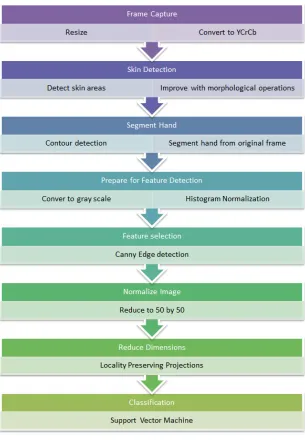
A critical task for this work was the development of a system to perform the task of training, processing and classifying ASL finger spelling. This is where the algorithm could be tested and developed with ease, while not worrying about the constraints of a mobile system and the extra difficulties of debugging code errors on the phone. In order to train this system, a reli-able database of imagery was created to provide the ground truth. Next the necessary training files for compression and classification were exported, and the method was implemented on the mobile device and corresponding server. The algorithm is displayed in a simplified form in Figure 3.1 show-ing each major step.
3.1
Algorithm
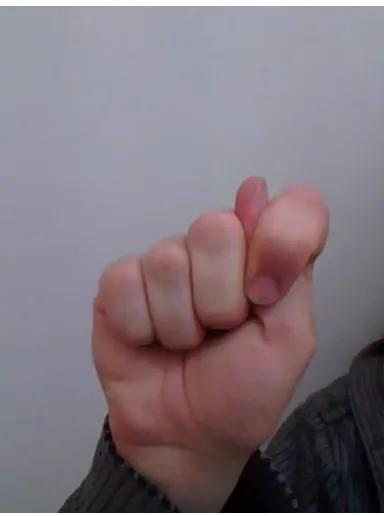
The algorithm begins with the initial scaling of the input image from the res-olution of 640 x 480 in Figure 3.2 to a 200 x 200 sized image with the cvRe-size method. It uses the CV INTER AREA parameter, which re-samples based on pixel area resolution preserving its original form.
cvResize (original image, scaled image, CV INTER AREA)
It was found early in development that processing the original image size was not necessary. There was not a significant effect on the classification accuracy, and it greatly improved the speed. Next the image is converted from its current color space to digitally encoded 8-bit YCrCb through the cvCvtColor method. The native computer system uses RGB video frames, but the mobile device has to convert from its own custom compressed ver-sion of analog encoded YUV in a 4-2-0 format. As with YCrCb color space the Y represents the luminance channel, and the U and V represent the chrominance (color) components. The particular 4-2-0 format defines the image frame to have as many Y components as pixels in the image but at
Figure 3.1: Process of Algorithm
1/4 the number of U and V components. Basically, there is one U and one V component for each two by two matrix of Y components. To get to the desired YCrCb color space, a direct conversion is not available, and thus sRGB color space is passed through.
Figure 3.2: Starting Frame
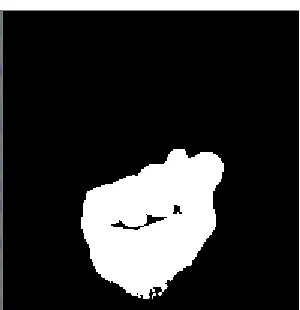
The image is then pushed through the custom skin detector with the thresh-old values shown in Section 2.2 for YCrCb color space. The resulting image is a binary mask that shows where the skin areas should be. In Figure 3.3a, the shape of the hand can be seen, but portions of the hand that are in shadow are missing when using the RGB method. In comparison the YCrCb method provides a complete detection of the hand shape in Figure 3.3b.
This image can easily consist of small areas of false positives due to compression artifacts and false negatives due to small shadows on the hand. In order to smooth out those imperfections, morphological operations of erosion and dilation are used from the operations of cvErode and cvDilate. First a kernel of 4 x 4 ellipse is used to erode the image to eliminate these small artifacts, leaving only the larger blobs in the mask as seen in Figure 3.4a. Then the same kernel of a 4 x 4 ellipse is used to fill in the gaps and accentuate the remaining edges as seen in Figure 3.4b.
(a) RGB binary skin mask (b) YCrCb binary skin mask
Figure 3.3: Skin Masks
(a) Erosion (b) Dilation
(a) Filled in around outer edge of largest contour blob
(b) Color segment of original frame
Figure 3.5: Contour Operations
With a few other skin mask blobs likely left behind, the largest blob is thus singled out through a contour detection method in cvFindContours and some post processing. It was set with the mode CV RETR EXTERNAL so that only the exterior contours of each blob were detected. The largest area contour is then sectioned out and filled in as shown in Figure 3.5a. It is then used to section out the hand from the original color image with a simple binary comparison as shown in Figure 3.5b.
cvFindContours(inputImage, memoryStorage, addressToFirstCon-tour, sizeOfConaddressToFirstCon-tour, mode, method);
Next, the hand image is converted to gray scale to prepare for the edge detection feature selection. However before edge detection, the image is put through a histogram normalization for the whole 0 to 255 spectrum in order to assist in adjusting for differences in lighting with the command cvNormalize. Canny edge detection is chosen as the final feature selector due to its ability to adjust separate thresholds for major and minor edges .
cvNormalize(inputImage, outputImage, lowerBound, upperBound, mode);
(a) Canny edge detection applied
(b) Edge image resized to 50x50
Figure 3.6: Canny edge detection
It can give the best significant detail by ignoring minor edges that are not connected to a major edge. In order to accomplish that, the Canny algorithm performs two passes over the image. The first pass uses a stricter threshold in order to only find the significant edges. The second pass has a lower threshold and detects only edges that are directly connected to a significant edge. Canny edge detection helps most in signs that have intricate detail in the middle of the hand, such as the position of each individual finger. This image can be seen in Figure 3.6a.
With the Canny edge detection applied, the 8-bit image is further com-pressed to a 50 x 50 pixel sized image through the same resize command, ready to be put through PCA or LPP. Figure 3.6b shows this smaller image, revealing the form of the hand is still preserved quite well. This is the point during the network method that this small 50 x 50 image is passed to the external server for the final classification. A simple Java socket passes these bytes straight to the server and then automatically begins to process another video frame.
The last step is to perform the reduction of dimensions by either PCA or LPP and then push the reduced data through its corresponding SVM clas-sification on the device or on the server. Though a 50 x 50 image seems
small, to the classifier it still consists of D = 2500 dimensions. The PCA
or LPP matrix will be cross multiplied with the small image to produce a single vector through the project command. The PCA matrix results in d=50
dimensions, and the LPP matrix results ind = 30dimensions. Next the
the result is displayed for the user, and various actions may be preformed like writing it into a text message or manipulating the music player to play or stop a song.
PCA: project(inputImage, outputImage); SVM: result = predict(featureVectors);
3.1.1 Variations from Main Method
A few variations to the algorithm were explored in the process of creat-ing this system. One variation was in dimensionality reduction technique, where PCA was selected first to compress the feature data before classifi-cation. Afterward LPP was used instead, and it was found that PCA did not separate the classes in the feature space as well as LPP, and it required around 50 dimensions on the output in order to get satisfactory results. An-other variation was in the choice of color space. First RGB skin segmenta-tion was used to find the skin areas. As stated before, it is more sensitive to lighting changes and shadows, and thus it was replaced with YCrCb discrete segmentation. Both of these variations are discussed in Section 2.1.
Figure 3.7: Rotation Areas
to minimize the number of variations of hand signs by eliminating the error incurred from rotations. The vector to determine the hand’s angle was deter-mined from the longest vector of the encompassing box, either the height or width, that surrounds the borders of the skin mask contour. If the vector was greater than 30 degrees off the vertical, it was rotated to match the vertical axis. This rule was the same for the horizontal axis. Anything in between these two cases was shifted to the diagonal axis as 45 degrees, between 30 and 60 degrees. These three rotation regions can be seen in Figure 3.7: the green is set to zero degrees, yellow is shifted to 45 degrees, and the red area is set to 90 degrees. The surrounding box is seen in Figure 3.8. In this fig-ure, the sign ”B” is tallest on its height and is around 15 degrees off center; thus, is will be rotated to match the vertical axis. There were certain signs that produced angles typically always on the borders between the 3 sections, thus causing them to vary too drastically in the feature space. Though the results of this algorithmic variation are unpredictable, it is reviewed in the results section. It was incorporated in the algorithm by observing the skin mask image and rotating it accordingly before the rest of the preprocessing is performed.
Figure 3.8: Detection of Sign Angle
detected, a simple vertical flip to the image will allow the system to func-tion. This is accomplished by reading in all the images of the right handed database into one class. The second class consists of the right handed im-ages flipped vertically, representing the left hand. With only two classes to classify, it becomes a simple linear kernel on a single SVM. This method follows the same preprocessing up to the 50 by 50 image as the sign classi-fication does. Only at this step is the image tested by the right or left hand classifier, and then the image is flipped before sign classification if it turns out that the user is using the left hand.
3.2
Native Computer System and Training
This section describes the database used to train the classification tools, the training system developed, classification testing programs and the strategies to explore the variations on the main method. Three separate programs are created: one to read the database and train the PCA, LPP and SVM; one to to test the algorithm on singular videos for real-time observation; and the last program to run the algorithm through a set of videos for each sign to perform classification verification.
3.2.1 Database
sensor. The arm of the model is covered to the wrist in a dark material, limiting skin exposure to just the hand. Multiple videos and images of the hand in each sign are taken in this aforementioned state at different angles, generally with not more than 15 degrees difference in both axes from the most frontal representation of the sign. The best single images and video frames are extracted and put in separate folders for each sign. Thus the training program can assume every image in each folder is associated with that respective sign. Together this represents the custom database for the mobile training.
Figure 3.9: Image of the letter L from the training database
As a subset of this database, some other videos were recorded where no frames for training are extracted. They are defined as the test set. These are used in order to validate the algorithm in the classification verification program.
3.2.2 Training
The program would first read in the images from the database and process them to place where they consist of only the features. This creates nor-malized 50 x 50 pixel images of the edges of the hand, right before it is pushed through a compression method. At this point the images are flat-tened to a single row with a column length of the number of pixels in the entire image, and then added together into a large matrix with a number of rows equal to the number of images in the database. A secondary vec-tor svec-tored the numerical ground truth labels of each row. An external text file defined the string representation of each sign, and the numerical label shows its position in the array. The signs consist of A to Z letters, a sign for a space character and delete operation and lastly music controls consist-ing of play, stop, next and previous. To train the PCA, the image is placed into the PCA constructor provided by OpenCV. It is set with the parameter CV PCA DATA AS ROW signifying the data as in a row and the desired number of output eigenvector components. This number of eigenvectors is determined by trial and error as satisfactory when no more dimensions have any significant increase in classification accuracy. Tests using 50, 100, 200 and the number equaling 98% of top eigenvalues were tested. Since the LPP training is done in MATLAB, the combined image is first exported to a PNG file. The PNG file is then imported into the MATLAB tool re-purposed by Ray Ptucha. It calls the LPP training method on the data and provides resultant eigenvector and eigenvalue matrix. The number of eigenvector components for LPP is determined by taking the top 99% of eigenvalues. These generated eigenvectors from PCA in the training tool and LPP from the MATLAB tool are exported as an XML file for later use.
Next the LPP XML are read back into the training program, and the training data is cross multiplied with both methods through projection (Eq. 2.14). This constructs the compressed feature space. In order to visualize the feature space after compression, the top three values of the result can be graphed. This is seen in Figures 3.10 and 3.11. Next the SVM is configured with specific parameters in order to best classify the data.
Figure 3.10: PCA feature space (Top 3 eigenvectors shown out of 50)
Figure 3.11: LPP feature space (Top 3 eigenvectors shown out of 30)
C SVC : An n-class classification with n ≥ 2. The classes may have
im-perfect separation, and a parameterC is a penalty for outliers.
NU SVC : Another imperfect separation n-class classification.The
param-eter nusmooths out the decision boundary. A larger nuvalue smooths
out the decision boundary even more.
EPS SVR : This classification performs regression, while giving a
parame-terpfor defining a maximum distance between the feature vectors and
the hyperplane. The penalty multiplier of C is also used for outliers.
NU SVR : This classification also performs regression, but only uses the
parameternufor distance between feature vectors and the hyper-plane.
ONE CLASS : A one-class SVM where all the features are from the same label. The feature vectors built separate the class from the rest of space.
The SVM type used in this project is NU SVC. It was required to have n-class classification for this application to allow imperfect separation, and
the nuparameter allows for a quick way to adjust the decision boundary. As
seen in Figures 3.10 and 3.11, the classes tend to intermix sometimes. Thus, boundaries should not be too strict, but large separation is achieved with a larger number of dimensions, (here 30 or 50).
The next setting is the kernel type, which transforms the input data with an equation before the support vectors are determined. The first is linear (2.15) , where there is no change to the data in, contrast to a polynomial (2.16) or radial basis function (2.17), which perform their respective con-versions to the input data. For this work, the radial basis function works the best, as it helps the circular clumps per class in the input data become much more separated. This is especially seen in Figure 3.11.
stop once it achieves an accuracy lower than this epsilon value. Thus by us-ing both values, the hard iteration limit will stop the algorithm from runnus-ing forever, but also will stop the algorithm before the maximum number of it-erations if it reaches a point where it is accurate enough. Then the OpenCV version of SVM with these settings is trained with this compressed feature data and the corresponding label vector. This trained SVM is also exported to an XML file.
3.2.3 Classification Testing
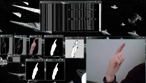
A second C++ program was used in order to test the developed algorithm instead of having to run it on the mobile device. It improved turnaround when changes were made to the algorithm. The input was a pre-recorded video from the mobile device. The process began by parsing the XML files for the SVM, PCA and LPP functions. Then it took each frame from the input, processed it with the aforementioned algorithm and classified it with the SVM. The output was displayed alongside many test output windows from each stage like skin and edge detection. An example of its output can be seen in Figure 3.12. In real time the results of using LPP over PCA could be seen, in addition to the effects of rotation or RGB skin detection.
3.2.4 Variations on Main Method
Figure 3.12: Example of the output from the testing software
Figure 3.13: PCA feature space with Rotation (Top 3 eigenvectors)
Figure 3.14: LPP feature space with Rotation (Top 3 eigenvectors)
[image:43.612.211.407.92.239.2]flipping the image on the vertical axis to mimic the other hand. For PCA, it uses the same settings as sign classification, but the SVM is slightly tweaked to adjust to its new feature space shown in Figure 3.15 as the top three results for each image. The SVM is instead a single binary classifier. Each class in the PCA feature space is largely clustered together so the separating plane will be placed directly between them. On the other hand, LPP needed only one dimension to determine the hand, shown in Figure 3.16. It will also use the binary classifier and is easily separable by a single value of zero. If the result after multiplication with the eigenvector is negative, it is one hand, whereas a positive result means it is the other.
Figure 3.16: LPP feature space of Left and Right Hand (Top 1 eigenvectors)
3.3
Mobile Device
The second part of this implementation is the mobile device. The appli-cation was developed to perform device-only classifiappli-cation or utilize the server to off-load a part of the algorithm. In Figure 3.17, the user interface for this application is shown. The bottom right corner contains the button for starting and stopping classification, while the left corner shows the cur-rent detected sign. When a sign is detected over the span of 3 frames it will be written in the middle bottom panel. At the top right a Wi-Fi sym-bol indicates whether there is a reliable connection to the external server. This can be pressed to reconnect if necessary. On the top left the question mark symbol provides a link to a help screen to assist with the application’s usage. The extra options button on the Android device is used to provide options to reconnect and switch between LPP and PCA compression on the fly. Additionally the verification test dialog (described later in this chapter) is accessible here too.
Figure 3.17: Example of the mobile interface
intensive portions are in native code in order to gain interoperability with OpenCV and hopefully gain a faster process.
Once the classifying button is pressed, a separate thread starts in the ap-plication that makes a call to the camera object to capture a singular frame. Then this singular frame, in bytes, is passed through the JNI to the C++ code underneath where it is to be processed by the aforementioned algo-rithm. The difference from the native computer application is that the color conversion requires a different parameter to accommodate the unique YUV format of the Android’s camera. Otherwise the rest of the algorithm is iden-tical up to the point where the compressed 50 x 50 edge detected image is finished. The network method on the mobile device continues the rest of the algorithm on the remote server.
480. Its data connection is at Max 3G, which provides a theoretical down-load speed of 14.4 Mbits/s and updown-load of 5.76 Mbits/s. For later analysis of the data usage for this research, the maximum download and upload speed can be interpreted as 1800 KBytes/s and 708.75 KBytes/s respectively.
3.3.1 Device-Only
This mode of the application continues to run LPP or PCA on the 50 x 50 image and then classifies the result with a trained SVM. In order to accom-plish this, the required XML files were preloaded onto the phone, and when the application was started, the files were read to create the objects. Thus in this mode the network is not required, a result is found in the C++ por-tion and then it is passed back the to user interface layer through JNI and displayed through the user interface thread.
3.3.2 Server Assisted
to display anything. When the mobile device’s networking thread receives classification data from the server, the mobile device uses the same logic as the device-only method to display the result.
In order to evaluate the real-time implementation of the algorithm, multiple test cases for both the computer system and mobile device were run. The native system was utilized to quickly test how well the classification per-forms in different conditions by using various videos taken by the mobile device. Additionally, settings like the number of eigenvectors from the com-pression of PCA and LPP were varied, or the effect of the rotation option was tested. These aforementioned tests measure the real time performance of the mobile application.
4.1
Classification Verification
A third desktop application was created to handle the reading of large num-bers of video image frames for verification. Different XML files are used to change the SVM or LPP settings. It steps through each video classify-ing the input and comparclassify-ing it to the known ground truth. At the end, the correct classifications per letter and overall classification accuracy are com-puted and placed into an external report. To do this testing, multiple videos are created using the mobile device’s camera to keep in line with the quality of imagery from a mobile device. These do not contain any images that are used for the database. Each trained sign has its own video where the hand is rotated to a max of 15 degrees in all three axes, with uniform lighting for each set. An example image from the verification video set is shown in Figure 4.1; it is well lit with some shadows and a semi cluttered background due to the user’s body.
The number of eigenvalues for PCA and LPP were varied for multiple tests in order to see the effect on the results and find a number that had the highest classification accuracy. The range of eigenvalues for PCA was from 50 to 200, as well as a number matching 98% of the largest eigenvalues. For LPP, the number matching 99% of the eigenvalues and a number half that
Figure 4.1: Example frame from verification videos showing the letter K
were used. Last but not least, the previously described rotation addition to the algorithm was tested to see if it was able to improve the classification accuracy.
4.2
Mobile Verification
button is pressed, the device will classify the incoming frames for the lim-ited amount of time and then automatically will calculate the classification accuracy based on the set sign from the dialog. This provides verification that the mobile device performs with results similar to the native computer system.
The next metric involves various time measurements. For instance in the cloud assisted method, the time for the image preprocessing is between when the frame is captured to the time it is ready to be transmitted. Network delay, (i.e., round trip time), is calculated from the time the image packet leaves for the server until a result for that frame returns. However for the device only case, the only measurement is from the frame capture point to when the frame is fully classified. There are other portions of the application that may affect the classification accuracy according to the point of view of the user, such as CPU dealing with other operations on the phone like the camera and system applications. Thus the number of classifications over the time classified is calculated to take into account all other factors. In order to minimize the effect of other processes causing variance in the performance of the application, the phone is reset just before the tests are taken for each set. This puts the phone close to the same state for every test, with the same background applications running every time.
The amount of energy in joules used by either implementation was mea-sured by an application called PowerTutor, which is available from the Google Play market. It is stated to be accurate to around 5% of actual values for supported phones, but it may give a rougher estimate on other devices. The energy used by the LCD screen, CPU, WiFi and 3G radios are deter-mined. The total power in watts is calculated by dividing the energy (J) by the time of operation.
private memory added to the shared memory that the application actually uses. Total shared memory for an application does not necessarily mean the application uses all of the available space; thus PSS determines the actual usage.
This chapter reports the multiple tests performed on both the mobile devices and on the classification verification system and analyzes their results. In the upcoming classification verification section, the following results were gen-erated from the tests previously described in Section 4.1. The computer pro-gram was used to test multiple videos for each defined sign, retrieving the classification accuracy per letter and average classification accuracy. They were held to the standard of no more than approximately 15 degrees rota-tion in all axes from a straight on view and kept uniform lighting per set. In order to test other changes to the system, the variations described in Section 3.1.1 were also verified while utilizing the optimal settings for the SVM, PCA or LPP from the original algorithm to allow a direct comparison. The mobile verification section follows the procedures defined in Section 4.2. The mobile verification methods not only test the classification rates of the application but also gather performance data such as time delays, power and memory usage. Both the native application mode and the cloud assisted method were tested, and their results were analyzed to determine the bene-fits and detriments of each method.
5.1
Classification Verification
The classification verification was run on a high end PC to measure clas-sification rates only. Some optimization of the algorithm was also pursued through analysis of the speed on the system in order to prepare for the lim-ited mobile device hardware. There are many tables showing the classifica-tion per letter in this secclassifica-tion, covering different settings to the LPP and PCA methods of dimensionality reduction.
Table 5.1: Classification Accuracy
Method Eigenvectors Average Classification Accuracy(%) Table
PCA 50 71.28 5.2
PCA 100 67.12 5.3
PCA 200 68.66 5.4
PCA 526 70.60 5.5
LPP 30 75.15 5.6
LPP 15 73.37 5.7
5.1.1 Classification Results for PCA and LPP
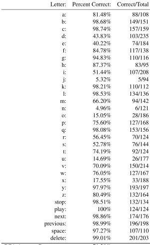
The first method of compression used in the project was principal compo-nent analysis (PCA). In order to find the best number of vectors to use, the verification tests were run using 50, 100 and 200 vectors. These results are seen in Tables 5.2, 5.3 and 5.4. Additionally, 526 vectors, (the number cor-responding to 98% of the highest eigenvalues), was also tested, as shown in Table 5.5. The lighting in this set was kept bright and the background mostly uncluttered to ensure the hand shape was captured. Table 5.1 shows the av-erage classification accuracy of PCA for varying numbers of eigenvectors. The best classification accuracy from PCA was 71% with 50 eigenvectors. A graph of the per letter tables can be seen in Figure 5.1.
Using different numbers of eigenvectors affected the classification rates for certain letters/signs, as seen especially with the PCA classification ta-bles. For example, the letter “e” is detected around 80% with 200 (Table 5.4) and 526 (Table 5.5) eigenvectors, but drops to 70% with 100 (Table 5.3) and to a low 40% with 50 (Table 5.2). This is likely due to the changes to the PCA feature space when reducing the number of eigenvectors. The changes are hard to visualize because we can only see 3 dimensions easily like in Figure 3.13.
with 15 eigenvectors, and the results summarized in Table 5.7 show only a 73% classification accuracy. It was only a small dip, but it shows that 30 eigenvectors are necessary for the highest classification accuracy observed in these tests. Thus the 30-dimensional SVM was incorporated in the mobile application.
Table 5.2: PCA Classification Per Letter w/ 50 eigenvectors
Letter: Percent Correct: Correct/Total
a: 81.48% 88/108
b: 98.68% 149/151
c: 98.74% 157/159
d: 43.83% 103/235
e: 40.22% 74/184
f: 84.78% 117/138
g: 94.83% 110/116
h: 87.37% 83/95
i: 51.44% 107/208
j: 5.32% 5/94
k: 98.21% 110/112
l: 98.53% 134/136
m: 66.20% 94/142
n: 4.96% 6/121
o: 15.05% 28/186
p: 75.60% 127/168
q: 98.08% 153/156
r: 56.45% 70/124
s: 52.78% 76/144
t: 74.19% 92/124
u: 14.69% 26/177
v: 70.09% 150/214
w: 76.05% 127/167
x: 17.55% 33/188
y: 97.97% 193/197
z: 80.49% 132/164
stop: 98.51% 132/134
play: 100% 124/124
next: 98.86% 174/176
previous: 98.99% 196/198
space: 97.27% 107/110
delete: 99.01% 201/203
Table 5.3: PCA Classification Per Letter w/ 100 eigenvectors
Letter: Percent Correct Correct/Total
a: 81.48% 88/108
b: 98.68% 149/151
c: 98.74% 157/159
d: 42.98% 101/235
e: 69.57% 128/184
f: 84.06% 116/138
g: 98.28% 114/116
h: 89.47% 85/95
i: 6.73% 14/208
j: 0% 0/94
k: 98.21% 110/112
l: 98.53% 134/136
m: 54.23% 77/142
n: 0% 0/121
o: 22.04% 41/186
p: 91.07% 153/168
q: 89.74% 140/156
r: 47.58% 59/124
s: 24.31% 35/144
t: 70.16% 87/124
u: 0% 0/177
v: 85.98% 184/214
w: 98.80% 165/167
x: 4.79% 9/188
y: 98.98% 195/197
z: 0% 0/164
stop: 98.51% 132/134
play: 100% 124/124
next: 98.86% 174/176
previous: 98.48% 195/198
space: 98.18% 108/110
delete: 99.01% 201/203
Table 5.4: PCA Classification Per Letter w/ 200 eigenvectors
Letter: Percent Correct: Correct/Total
a: 76.85% 83/108
b: 98.68% 149/151
c: 98.74% 157/159
d: 50.21% 118/235
e: 82.61% 152/184
f: 84.78% 117/138
g: 98.28% 114/116
h: 94.74% 90/95
i: 38.46% 80/208
j: 0% 0/94
k: 98.21% 110/112
l: 98.53% 134/136
m: 76.06% 108/142
n: 1.65% 2/121
o: 17.20% 32/186
p: 80.36% 135/168
q: 96.15% 150/156
r: 49.19% 61/124
s: 9.03% 13/144
t: 66.94% 83/124
u: 0% 0/177
v: 84.58% 181/214
w: 92.81% 155/167
x: 2.13% 4/188
y: 95.43% 188/197
z: 0% 0/164
stop: 98.51% 132/134
play: 100% 124/124
next: 98.86% 174/176
previous: 98.48% 195/198
space: 98.18% 108/110
delete: 99.01% 201/203
Table 5.5: PCA Classification Per Letter w/ 526 eigenvectors (98%)
Letter: Percent Correct: Correct/Total
a: 68.52% 74/108
b: 98.68% 149/151
c: 98.74% 157/159
d: 50.64% 119/235
e: 84.78% 156/184
f: 84.78% 117/138
g: 89.66% 104/116
h: 97.89% 93/95
i: 62.02% 129/208
j: 0% 0/94
k: 98.21% 110/112
l: 98.53% 134/136
m: 67.61% 96/142
n: 0% 0/121
o: 13.98% 26/186
p: 97.02% 163/168
q: 97.44% 152/156
r: 83.87% 104/124
s: 13.89% 20/144
t: 62.10% 77/124
u: 1.13% 2/177
v: 79.91% 171/214
w: 98.20% 164/167
x: 2.66% 5/188
y: 95.94% 189/197
z: 0% 0/164
stop: 98.51% 132/134
play: 100% 124/124
next: 98.86% 174/176
previous: 98.48% 195/198
space: 98.18% 108/110
delete: 99.01% 201/203
Table 5.6: LPP Classification Per Letter w/ 99% of highest eigenvectors (30)
Letter: Percent Correct: Correct/Total
a: 58.33% 63/108
b: 94.70% 143/151
c: 91.82% 146/159
d: 76.17% 179/235
e: 97.28% 179/184
f: 94.93% 131/138
g: 89.66% 104/116
h: 94.74% 90/95
i: 94.71% 197/208
j: 0% 0/94
k: 98.21% 110/112
l: 98.53% 134/136
m: 78.87% 112/142
n: 4.96% 6/121
o: 37.63% 70/186
p: 89.88% 151/168
q: 98.08% 153/156
r: 83.87% 104/124
s: 31.25% 45/144
t: 80.65% 100/124
u: 34.46% 61/177
v: 64.02% 137/214
w: 98.20% 164/167
x: 32.45% 61/188
y: 95.94% 189/197
z: 0.61% 1/164
stop: 98.51% 132/134
play: 100% 124/124
next: 88.07% 155/176
previous: 76.77% 152/198
space: 69.09% 76/110
delete: 97.54% 198/203
Table 5.7: LPP Classification Per Letter w/ eigenvectors (15)
Letter: Percent Correct: Correct/Total
a: 92.59% 100/108
b: 98.01% 148/151
c: 88.68% 141/159
d: 62.55% 147/235
e: 97.83% 180/184
f: 73.19% 101/138
g: 98.28% 114/116
h: 72.63% 69/95
i: 96.63% 201/208
j: 0% 0/94
k: 98.21% 110/112
l: 94.12% 128/136
m: 7.04% 10/142
n: 2.48% 3/121
o: 48.92% 91/186
p: 95.83% 161/168
q: 98.08% 153/156
r: 87.90% 109/124
s: 27.78% 40/144
t: 63.71% 79/124
u: 1.69% 3/177
v: 30.84% 66/214
w: 98.80% 165/167
x: 47.87% 90/188
y: 98.98% 195/197
z: 71.34% 117/164
stop: 98.51% 132/134
play: 100% 124/124
next: 98.86% 174/176
previous: 79.29% 157/198
space: 66.36% 73/110
delete: 98.03% 199/203
5.1.2 Classification Results for Rotation Variation
First, the explored method of rotation was tested for improvement with the results shown in Table 5.8. 30 eigenvectors were used for LPP, and 98% of the highest eigenvectors for PCA was used. From these tests, it seems the results were much worse with accuracy of 55% for PCA and 46% for LPP, and thus this variation was not included in the primary algorithm. The main issue with this method is that certain signs tended to be on the borders between the 3 areas of horizontal, diagonal and vertical. This caused the features of one sign to reside sometimes in two separate places in the feature space. Additionally some signs may be rotated and thus become too close to each other in the feature space.
5.1.3 Classification Results for Hand Detection Variation
Table 5.8: LPP (30) and PCA (526) Classification Per Letter with Rotation
Letter: PCA: Correct: PCA:Correct/Total: LPP: Correct: LPP:Correct/Total:
a: 48.15% 52/108 53.70% 58/108
b: 98.01% 148/151 87.42% 132/151
c: 98.74% 157/159 88.05% 140/159
d: 45.96% 108/235 45.96% 108/235
e: 25% 46/184 54.89% 101/184
f: 60.14% 83/138 63.04% 87/138
g: 3.45% 4/116 6.03% 7/116
h: 89.47% 85/95 31.58% 30/95
i: 17.31% 36/208 22.12% 46/208
j: 95.74% 90/94 11.70% 11/94
k: 5.36% 6/112 3.57% 4/112
l: 98.53% 134/136 91.18% 124/136
m: 0% 0/142 2.82% 4/142
n: 2.48% 3/121 3.31% 4/121
o: 13.44% 25/186 8.06% 15/186
p: 51.79% 87/168 0% 0/168
q: 83.33% 130/156 83.97% 131/156
r: 33.87% 42/124 36.29% 45/124
s: 1.39% 2/144 2.08% 3/144
t: 19.35% 24/124 25.81% 32/124
u: 38.42% 68/177 16.38% 29/177
v: 63.55% 136/214 64.95% 139/214
w: 79.04% 132/167 43.71% 73/167
x: 0% 0/188 2.66% 5/188
y: 93.91% 185/197 86.29% 170/197
z: 0% 0/164 0% 0/164
stop: 98.51% 132/134 97.76% 131/134
play: 100% 124/124 79.84% 99/124
next: 98.86% 174/176 87.50% 154/176
previous: 93.94% 186/198 67.68% 134/198
space: 96.36% 106/110 71.82% 79/110
delete: 99.01% 201/203 86.70% 176/203
Table 5.9: Hand Classification with LPP(1) and PCA(200)
Letter: PCA Right Hand PCA Left Hand LPP Right Hand LPP Left Hand
a: 87.03% 87.03% 87.96% 87.96%
b: 90.72% 45.03% 84.10% 84.10%
c: 98.74% 98.11% 84.90% 84.90%
d: 96.17% 95.31% 70.63% 70.63%
e: 97.82% 97.82% 88.58% 88.58%
f: 98.55% 78.98% 97.82% 97.82%
g: 98.27% 98.27% 98.27% 98.27%
h: 92.63% 96.84% 84.21% 84.21%
i: 43.75% 57.69% 41.34% 41.34%
j: 96.80% 85.10% 3.19% 3.19%
k: 98.21% 98.21% 94.64% 94.64%
l: 97.79% 98.52% 97.79% 97.79%
m: 92.25% 91.54% 38.73% 38.73%
n: 98.34% 90.08% 74.38% 74.38%
o: 97.84% 97.84% 86.02% 86.02%
p: 98.21% 98.80% 95.23% 95.23%
q: 55.76% 69.87% 85.89% 85.89%
r: 55.64% 74.19% 28.22% 28.22%
s: 93.05% 97.91% 95.13% 95.13%
t: 97.58% 84.67% 73.38% 73.38%
u: 92.65% 92.65% 49.71% 49.71%
v: 98.59% 98.59% 96.72% 96.72%
w: 98.80% 98.80% 76.64% 76.64%
x: 98.40% 98.40% 73.93% 73.93%
y: 98.98% 95.43% 74.61% 74.61%
z: 98.17% 98.17% 98.17% 98.17%
stop: 98.75% 98.50% 87.31% 87.31%
play: 100.00% 100.00% 83.87% 83.87%
next: 96.27% 98.86% 65.90% 65.90%
previous: 67.17% 63.13% 66.16% 66.16%
space: 85.45% 88.18% 75.45% 75.45%
delete: 97.53% 97.04% 80.29% 80.29%
5.2
Mobile Verification
This section presents the mobile device tests involving the classification ac-curacy, various timing calculations, memory usage and power usage. The desired result is a system that matches or exceeds the classification accuracy of the computer verified system while achieving a classification speed above 2 frames per second. Additionally, the cloud assisted application seeks to increase the classification speed, while reducing memory usage and not in-creasing the power usage.
5.2.1 Classification Accuracy
Table 5.10: Native and Mobile Classification Rates per Letter
Sign: Native: Percent (%) Frames Classified Cloud: Percent (%) Frames Classified
a 88.75 80 95.69 93
b 100.00 66 99.10 112
c 100.00 48 91.54 71
d 100.00 58 94.36 71
e 89.79 49 100.00 71
f 100.00 47 92.95 71
g 91.35 81 86.30 73
h 76.27 59 66.66 72
i 88.67 53 86.11 72
j 86.88 61 60.56 71
k 100.00 51 79.41 68
l 98.27 58 95.89 73
m 80.64 62 44.28 70
n 1.16 86 86.30 73
o 1.29 77 2.73 73
p 100.00 84 94.28 70
q 76.92 91 27.77 72
r 71.95 82 49.33 75
s 1.12 65 56.16 73
t 54.05 74 46.47 71
u 3.38 59 45.71 70
v 68.00 50 94.44 108
w 86.79 53 89.71 107
x 58.62 58 62.93 116
y 72.54 51 79.25 108
z 73.07 52 50.43 115
play 100.00 49 87.95 83
stop 100.00 46 90.54 74
next 92.15 51 92.85 70
previous 96.36 55 80.30 66
delete 56.89 58 100.00 92
space 94.33 53 82.53 63
5.2.2 Timing
Various timings were measured to contrast cloud-assisted versus solely local processing in order to judge the application’s performance. In order to get the processing time and network delay, a system of timestamps was recorded for each sign classified. For example, Table 5.12 and Table 5.11 show the time at three different places in the algorithm. The time in start column time was recorded just after a frame from the camera was pulled for either the native or cloud method. The send column time was registered either right after classification was completed (in the native method) or right after preprocessing (before sending to the server in the cloud method). Lastly the receive column time was used only by the cloud method to record when the result returned from the server. The exact amount of processing done on the mobile device was calculated as the difference between the start and send times. The round trip time (RTT) time was calculated as the difference between the send and receive times.
Table 5.11: Native method Timestamps
Start: Send: Receive: Processing Time: Letter:
19:08:26::332 19:08:26::425 00:00:00::000 00:00:00::093 a 19:08:26::725 19:08:27::025 00:00:00::000 00:00:00::300 a 19:08:27::074 19:08:27::163 00:00:00::000 00:00:00::089 a 19:08:27::208 19:08:27::307 00:00:00::000 00:00:00::099 a 19:08:27::626 19:08:27::814 00:00:00::000 00:00:00::188 a 19:08:27::862 19:08:28::427 00:00:00::000 00:00:00::565 a
Table 5.12: Cloud method Timestamps
Start: Send: Receive: Processing Time: RTT Time Letter:
15:19:55::092 15:19:55::202 15:19:55::528 00:00:00::110 00:00:00::326 a 15:19:55::816 15:19:56::047 15:19:56::398 00:00:00::231 00:00:00::351 a 15:19:56::361 15:19:56::475 15:19:56::805 00:00:00::114 00:00:00::330 a 15:19:56::823 15:19:56::911 15:19:57::297 00:00:00::088 00:00:00::386 a 15:19:57::239 15:19:57::369 15:19:57::701 00:00:00::130 00:00:00::332 a 15:19:57::705 15:19:57::871 15:19:58::189 00:00:00::166 00:00:00::318 a
![Figure 2.2: Radial basis kernel [20]](https://thumb-us.123doks.com/thumbv2/123dok_us/47007.4242/22.612.128.487.92.375/figure-radial-basis-kernel.webp)