City, University of London Institutional Repository
Citation
:
Evans, A. and Schäfer, A. (2013). The Rebound Effect in the Aviation Sector. Energy Economics, 36, pp. 158-165. doi: 10.1016/j.eneco.2012.12.005This is the unspecified version of the paper.
This version of the publication may differ from the final published
version.
Permanent repository link:
http://openaccess.city.ac.uk/2088/Link to published version
:
http://dx.doi.org/10.1016/j.eneco.2012.12.005Copyright and reuse:
City Research Online aims to make research
outputs of City, University of London available to a wider audience.
Copyright and Moral Rights remain with the author(s) and/or copyright
holders. URLs from City Research Online may be freely distributed and
linked to.
1
The Rebound Effect in the Aviation Sector
Antony Evansa,c, Andreas Schäferb,c
aCorresponding author, City University London, Northampton Square, London EC1V 0HB, UK,
[email protected], Tel.: +44-(0)207-040-4118
bPrecourt Energy Efficiency Center, Stanford University, Yang & Yamazaki Environment &
Energy Building, 473 Via Ortega, Room 387, Stanford, CA 94305-4205, USA,
[email protected], Tel. +1-650-723-0884
cAviation Integrated Modeling Group, Institute for Aviation and the Environment, Martin Centre
for Architectural and Urban Studies, University of Cambridge, 1-5 Scroope Terrace, Cambridge,
2
Abstract1
The rebound effect, i.e., the (partial) offset of the energy efficiency improvement potential due to a
reduction in marginal usage costs and the associated increase in consumer demand, has been
extensively studied for residential energy demand and automobile travel. This study presents a
quantitative estimate of the rebound effect for an air traffic network including the 22 busiest
airports, which serve 14 of the highest O-D cities within the domestic U.S. aviation sector. To
satisfy this objective, passenger flows, aircraft operations, flight delays and the resulting energy use
are simulated. Our model results indicate that the average rebound effect in this network is about
19%, for the range of aircraft fuel burn reductions considered. This is the net impact of an increase
in air transportation supply to satisfy the rising passenger demand, airline operational effects that
further increase supply, and the mitigating effects of an increase in flight delays. Although the
magnitude of the rebound effect is small, it can be significant for a sector that has comparatively
few options for reducing greenhouse gas emissions.
Keywords
Rebound effect, aviation, energy use, greenhouse gas emissions
1Abbreviations
ATA – Air Transport Association
BADA – Base of Aircraft Data
DOT – U.S. Department of Transport ATA – Air Transport Association
BADA – Base of Aircraft Data
DOT – U.S. Department of Transport
IATA – International Air Transport Association
ICAO – International Civil Aviation Organization
O-D – True origin-ultimate destination
3
JEL Classification Codes
L93 Industry Studies: Air Transportation; R41 Transportation: Demand, Supply; Q55
Environmental Economics, Technological Innovation
1. Introduction
When introducing more fuel efficient technology into consumer or producer markets, the full
energy savings potential can often not be exploited, as the reduction in marginal costs generates
extra demand for energy services. This “rebound” effect or “take back” effect, first quantified for
household appliances by Khazzoom (1980), has mainly been studied for residential fuel demand,
household space heating and cooling, and automobile travel (Greening et al., 2000). For automobile travel, the rebound effect, defined here as the percentage offset of the reduction in energy use as
offered by the more fuel-efficient technology alone, was estimated to range from 10 to 30% (Greene
et al., 1999; Greening et al., 2000)2.
Understanding the magnitude of the rebound effect is especially important for aviation, given the
rapid growth of this sector and the comparatively limited opportunities for reducing greenhouse gas
emissions. Because of the constrained availability of synthetic low-carbon fuel substitutes (Schäfer
et al., 2009), even a small rebound effect can significantly increase the costs for mitigating aviation
2 Greene et al. (1999) and Greening et al. (2000) define the rebound effect as a percentage increase in energy services,
i.e., automobile driving, in response to a decrease in vehicle fuel consumption. Because kilometers driven are
proportional to energy use for a given automobile, driving cycle, and ambient conditions, this energy service related
rebound effect is identical to the energy use related rebound effect. The situation is different for space heating or
4
greenhouse gas emissions. When introducing a fleet of more fuel-efficient aircraft, the marginal
costs of operating these vehicles decline. Because of the competitive nature of the airline industry
within the network we study, any decline in operating costs would lead to reduced fares. As a
response to the reduction in fare, passengers would be expected to consume more air travel. Given
already high average passenger load factors of over 80% (DOT, 2010), this consumer adjustment,
which is determined by the price elasticity of air travel, is likely to be complemented by changes in
airline behavior. The decline in operating costs and (associated) increase in travel demand would
cause the airline industry to undertake various adjustments, including a change in flight network,
the use of differently sized (typically larger) aircraft, and—most importantly—an increase in flight
frequency (Evans and Schäfer, 2011). Along competitive routes, airlines battle for market share on
the basis of flight frequency (Belobaba, 2006)—an extra return flight a day gives passengers more
flexibility at what time to leave from and return to the point of origin. Any of these operational
changes translates into a change in energy use (the firm-related direct rebound effect). At the same
time, the extent of operational changes is limited by a potential increase in airport congestion and
thus flight delays, an outcome that increases airline operating costs and mitigates the increase in
passenger demand and thus the rebound effect.
This paper estimates the direct rebound effect for the U.S. domestic aviation sector, by taking into
account the above described adjustments on both the consumer and firm sides that lead to a new
equilibrium. We define the rebound effect in terms of energy use, i.e., the offset in energy use from
the technological potential due to a reduction in marginal costs leading to partial equilibrium
adjustments. As with the vast majority of rebound effect studies, we focus on the direct rebound effect. Studying the indirect rebound effect, which results from the increase in consumer purchasing
5
services (that also consume energy), and the resulting economy-wide adjustments would require the
use of computable general equilibrium models and are thus not considered here.
We continue with a detailed description of our model, which simulates the various adjustment
mechanisms described above. After validating the model, we estimate the magnitude of the rebound
effect for a network of U.S. airports. We then continue with testing the sensitivity of the results
before deriving conclusions.
2. Modeling Approach
To estimate the rebound effect in the aviation sector, passenger and airline behavior are simulated in
response to the introduction of low fuel burn technology. An integrated framework that captures the
interactions between the airline and passenger responses, ensuring that the simulation model
accounts for demand effects, changes in airline operations, and the impact of airport capacity
6
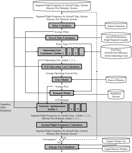
Figure 1. Modeling framework for simulating airline and passenger responses to lower fuel burn
technology. Frequency Game Simulation Demand Model O-D Demand
Operating Cost: Airline 1, 2, 3, ... Average Delay
Travel Time
Segment Flight Frequency by Aircraft Type: System Itinerary Pax Demand: System
Convergence? No Yes
Segment Flight Frequency by Aircraft Type: System Itinerary Pax Demand: System
Operating Cost Calculator: Airline 1
Segment Flight Frequency by Aircraft Type : Airline 1, 2, 3, ... Itinerary Pax Demand: Airline 1, 2, 3, ...
Travel Time Calculator
System Flight Frequency Calculator Fare Model
Average Fare
O-D Operating Cost Calculator
Average Operating Cost per Pax Segment Flight Frequency by Aircraft Type0: System
Itinerary Pax Demand0: System
Airport Capacities
Aircraft Performance Flight Segment Lengths
Population Income Fuel Price Aircraft Fuel Efficiency Airline Operating Costs
Energy Use Calculator
System Energy Use
Rates of Return0
Engine Energy Use
Flight Mission Profiles Delay Calculator
... 2 3
... 2 3 Network Optimisation:
7
Introducing lower fuel burn technology into the air transport system will in most cases reduce
airline operating costs. The latter, which include direct and indirect operating costs, are calculated
by Operating Cost Calculators for each airline. Direct operating costs, per flight hour, are
modeled for three aircraft types (small, medium and large), and two age categories (certified before
and after 1995), for each airline. Because equipage and operational practices differ by airline and
route, average direct operating costs are also airline and route-specific. With the exception of fuel
and oil costs and landing fees, all direct operating costs are estimated according to costs per flight
hour from U.S. Department of Transport Form 41 data, by aircraft type and airline (DOT, 2005),
and delays and travel times estimated by Delay and Travel Time Calculators, which are described
in Appendix A. Fuel costs are calculated independently according to fuel prices from the Air
Transport Association (ATA, 2008), and aircraft fuel burn rates in each phase of flight extracted
from the Base of Aircraft Data (BADA), an aircraft performance model developed by
EUROCONTROL (2004), and the Aircraft Engine Emissions Databank (ICAO, 2007). Landing
fees for each airport are input directly from the International Air Transport Association’s (IATA)
Airport and Air Navigation Charges Manual (IATA, 2008). Average operating costs per true
origin-ultimate destination (O-D) passenger are also calculated, by the O-D Operating Cost Calculator,
across all airlines, for input into a Fare Model.
The operating costs are translated into airfares by the Fare Model (see Figure 1). Pricing within the
airline industry has changed significantly over the past decades with the development of
computerized revenue management systems, web-based airline ticket distribution and on-line travel
agents (Carrier, 2006). As a result, airlines do not simply employ cost-based pricing, but apply a
combination of cost-, demand-, and service-based pricing, applying price discrimination and
8
applied directly to airline ticket pricing (e.g., Belobaba, 1989), but are highly complex, and not
tailored for use in aviation system models. Most aviation system models instead allow users to
specify airline yields or operating profits (e.g., Wingrove et al., 1998), or estimate cost pass-through to fares (e.g., Pulles et al., 2002), and do not explicitly model fare competition. We adopt this approach because fare competition is not a key driver of flight frequency, network, and aircraft size
choice, which drive system energy use. In this paper, we model average fares for each O-D market
separately by scaling the respective airline operating costs per O-D passenger with the year 2005
rate of return (the ratio of average fare and operating cost per passenger) for that market. This
approach, also pursued by Waitz et al. (2006), is transparent and results in better estimates of fares compared to the assumption that fares equal marginal operating costs (a 0% rate of return) given
cross-subsidies across markets3. The rate of return does not vary significantly across the simulated
network, evidenced by a tight linear relationship between observed operating cost per revenue
passenger kilometer (RPK) and observed yield (fare per kilometer) (R-squared of 0.96). The
corresponding network-wide rate of return is a low 4%, suggesting that these markets experience
high fare competition. Table 1 summarizes observed indicators of fare competition within the
simulated air traffic network, showing that when the number of competitors is three or greater,
which represents the majority of city pairs studied and the vast majority of RPK flown in the
studied network, average fares are well below those associated with fewer competitors, indicating a
high degree of fare competition.
3 We use average operating costs because marginal operating costs can be discontinuous and vary significantly
9
Table 1. Observed Indicators of Fare Competition within the Studied Flight Network
1 Competitor 2 Competitors Competitors 3 or more Total or Average
O-D Pairs 20 52 110 182
Seat-km (bln) 13 41 146 200
Average Fare (US$) 213 208 175 188
A reduction in airfares due to the adoption of lower fuel burn technology will result in an increase
in travel demand. The impact of air fares and other determinants on O-D passenger demand
between cities is estimated by a Demand Model (see Figure 1) using a one-equation gravity-type
model as described and applied by Reynolds et al. (2007). Income4 and population are key factors driving the demand for air travel (Battersby & Oczkowski, 2001; Corsi, Dresner, & Windle, 1997;
Mumayiz & Pulling, 1992), while travel time and flight delay are important "resistances” (Forbes,
2008, Kostiuk et al., 1998, Morrison & Winston, 1989). We also include flight frequency as an
explanatory variable, because of the demand impact of frequency competition, described below.
Because the rebound effect likely differs between leisure and business travel, the O-D passenger
demand should in theory be estimated for these markets separately. However, no recent data set
exists that would break down air passenger trips into these segments. This is further complicated by
recent trends showing that business and leisure travelers no longer typically travel in business and
leisure class, respectively. For these reasons, even airlines are no longer able to make accurate
estimates of business/leisure splits (Belobaba, 2011, personal correspondence). Equation 1
describes the demand model employed in this study.
4 Ideally, the income of air travelers should be used in the demand equation. However, most often these numbers are not
10
𝑙𝑛 𝐷!,! = 𝐶+𝛼∙𝑙𝑛 𝑃! ∙𝑃! +𝛾∙𝑙𝑛 𝐼! ∙𝐼! +𝛽∙𝑙𝑛 𝐹𝑙𝑡𝑓𝑟𝑒𝑞!,! +𝛿∙𝐴!,!+𝜇∙𝐵!,!+𝜑∙𝑆!,!+
𝜏∙𝑙𝑛 𝐹𝑎𝑟𝑒!,!+𝜃!∙𝑇!,! +𝜃! ∙𝐷𝑒𝑙𝑎𝑦!,! (1)
In equation 1, Dij represents the O-D passenger demand between cities i and j; C is a constant; P is
the related greater metropolitan area or equivalent population; I is the greater metropolitan area per capita income; Fltfreq is the estimated city-pair flight frequency, A is a binary variable indicating whether either city in the city pair has special attributes (e.g. a city being a major tourist destination
or capital); B is a complementary binary variable indicating whether either city does not have special attributes (both variables A and B are necessary to account for origin and destination city properties); S is a binary variable indicating whether road transport between the city pair is competitive with air transport (specified according to a distance-based criterion of 150 nautical
miles (278 km)) (Sij=1 if city i and j are less than 150 nm apart); is passenger airfare between
the cities averaged over all itineraries; θ1 is the passenger value of (nominal5) travel time; is the
nominal travel time between the cities averaged over all itineraries; θ2 is the passenger value of
delay time; and is the average flight delay between the cities averaged over all itineraries.
The exponents represent the elasticity of demand to each of the explanatory variables (in the case of
population and income, the elasticity of demand with respect to population and income is
represented by 2α and 2γrespectively). The final expression in brackets, which represents the
generalized costs to an intercity passenger, includes the demand effect of changes in fares, nominal
travel time (applying a passenger value of time) and flight delay (applying a passenger value of
delay). The passenger value of time was set to US$ 35 per hour, which is consistent with Dray et al.
5 Nominal travel time refers to unimpeded travel time, i.e., with no flight delay. Fare
T
11
(2010) and within the range estimated by U.S. DOT (1997). Passenger value of delay time (θ2) was
fixed at three times the passenger value of nominal travel time, as suggested by a comparison of
passenger values of travel time and delay time in the literature (U.S. DOT, 1997; Forbes, 2008).
Because of possible endogeneity with flight frequency, equation 1 was estimated using both
ordinary least squares (OLS) and two-stage least squares (2SLS) regression. In the latter case, the
instruments for the reduced form equation for flight frequency included the number of airlines
serving a city pair, the related total number of airports, and a binary variable indicating if both cities
in the pair have a hub airport. All instrumental variable coefficients were found to be of the
expected sign and significant at the 95% confidence level.6
The resulting coefficients of the OLS regression and of the second stage of the 2SLS regression are
reported in Table 2, along with their t-statistics. All parameters are significant at the 95%
confidence level, and compare well to the parameters estimated by Jamin et al. (2004) and Dray et al. (2010). The estimated coefficients of the OLS and 2SLS regressions are similar. Therefore, not surprisingly, the Hausman statistic has a small value of 0.13. We thus cannot reject the
Null-hypothesis that the difference in coefficients is not systematic and continue working with the OLS
based coefficients.
Table 2. Parameter estimates and t-statistics (in parenthesis) for the demand equation (N = 182
observations)
6 The data sources underlying these estimates for the United States in 2005 include DOT (2005), DOT (2007), U.S.
12
OLS 2SLS
Adjusted R2 0.874 0.873
Population (α) 0.842 (8.2) 0.867 (7.0)
Income (γ) 1.538 (4.7) 1.586 (4.5)
Flight Frequency (β) 0.192 (4.0) 0.171 (2.3)
Both cities have special attributes (δ) 0.368 (5.6) 0.366 (5.6) No city has special attributes (µ) -0.376 (-5.6) -0.376 (-5.6) Competitiveness of road transport (φ) -3.787 (-22) -3.803 (-21)
Generalized Cost (τ) -0.599 (-4.7) -0.640 (-3.7)
Constant -14.184 (-3.8) -14.639 (-3.7)
Because the value of time was specified exogenously, we tested the associated sensitivity of the
parameter estimates. Doubling the passenger value of time to $70 per hour results in the coefficients
changing by up to 5%, with the exception of the generalized cost elasticity, which declines by 17%.
The adjusted R-squared declines slightly from 0.874 to 0.869. Halving the passenger value of time
to $17.5 per hour also results in the parameters changing by a maximum of 5%, with the exception
of the generalized cost elasticity, which increases by 11%. The adjusted R-squared increases
slightly to 0.878.
An increase in passenger demand as a result of declining air fares will induce airlines to increase the
supply of air transportation services. To quantify the associated changes in flight frequencies,
aircraft size, and flight network within a competitive environment, a Nash best response game7
7 In game theory, the best response is the strategy (or strategies) which produces the most favorable outcome for a
player, taking other players' strategies as given (Fudenberg & Tirole, 1991, p. 29). A Nash equilibrium is the point at
which each player in a game has selected the best response (or one of the best responses) to the other players' strategies
13
modeling frequency competition is simulated in which profits are maximized by each airline. This
optimization is solved separately for each airline using a sequence of Network Optimizations (see
the lower part of Figure 1). These are solved within an iterative scheme simulating a myopic best
response dynamic game until convergence to a Nash equilibrium, which captures the effects of
frequency competition between airlines. This approach is described in detail by Evans (2010). The
airline objective function, which is presented in equation 2, consists of a revenue term and two cost
terms, the latter two representing airline costs per flight and per passenger.
(2)
In equation 2, represents the fare between O-D city pair i and j, averaged over all itineraries and airlines; Paxi,j,p,a represents passenger demand between O-D city pair i and j, on itinerary p, for
airline a; Costf m,n,k,a represents average cost per flight on the flight segment between airports m and n, for aircraft type k, for airline a; Fltfreqm,n,k,a represents the average number of flights per day on
the flight segment between airports m and n, using aircraft type k, for airline a; and CostP i,j,a
represents average cost per passenger between O-D city pair i and j, for airline a. Pi,j,a represents the
set of all passenger itineraries p between cities i and j operated by airline a; Citiesa represents all
cities served by airline a; Airportsa represents all airports served by airline a; SizeClassesa
represents all aircraft types operated by airline a, and Airlines represents the set of all airlines modeled. Airlines a Pax Cost Fltfreq Cost Pax Fare Cities
i j Cities p P
a p j i a j i p Airports
m Airports k SizeClasses
a k n m a k n m f Cities
i j Cities p P
a p j i j i
a ija
a a a
a a ija
14
Because fare competition is not a key driver of flight frequency, network, and aircraft size choice,
average O-D fares are determined exogenously to the optimization, and are input from the Average
Fare Model (see the middle of Figure 1). Passenger itinerary demand is a decision variable of the
objective function, with no passenger itinerary choice modeled – a reasonable simplification if
applied to a network serving predominantly non-stop passengers, such as that analyzed in this
paper. Average costs per flight (Costf m,n,k,a) and per passenger (CostP i,j,a) are input from the
Operating Cost Calculator for each airline (see middle of Figure 1). Segment flight frequency is also
a decision variable of the objective function, which, with passenger itinerary demand, incorporates
sufficient information to completely describe the airline daily flight frequency, fleet composition,
flight network, and passenger itinerary routing. Segment flight frequency is constrained to integer
values, per day, so the network optimization is solved as a Mixed Integer Program.
The objective function is constrained by a system of linear equations describing airline routing and
scheduling requirements along with system constraints. A seat constraint limits the number of
passengers served on each flight segment in the objective function to be less than or equal to the
number of seats available, with a maximum allowable load factor of 95%. The number of seats
offered by the airline is a direct function of the aircraft seating capacity and the flight frequency
offered. In addition, an airport balance constraint limits the number of flights of each aircraft type
departing from an airport per day to equal the number of flights of that aircraft type arriving, and
vice versa. A demand constraint is also included, limiting the demand served by any given airline to
be the proportion of the total available demand defined by the market share of that airline. Airline
market share is modeled by the ratio of the non-stop flight frequency offered between the cities by
15
each airline’s network optimization, the flight frequency of all other airlines, which is input from
the System Flight Frequency Calculator, is taken as constant. During each iteration step and for
any O-D pair, each airline increases its flight frequency to gain more market share, until the
marginal cost of adding another flight is greater than the marginal revenue associated with the
increased market share achieved by the flight. Since airlines experience different operating costs,
those with the lowest costs can add more extra flights and thus gain more market share.
System energy use is calculated by an Energy Use Calculator in each flight phase: ground idle,
taxi, take-off, climb-out, cruise, airborne holding, descent, approach and landing. Energy use is
calculated directly using fuel burn rates from BADA (EUROCONTROL, 2004) for each of the
aircraft types modeled. The duration of each phase of flight is input from the Travel Time
Calculator. System-wide energy use is calculated as a function of system and airport operations,
which are outputs of the iterative framework described above.
3. Model Validation
The model described in Figure 1 was validated by reproducing observed airline flight frequencies,
aircraft size choices and flight network choice for a network of 22 airports in the United States in
2005, using 2005 population, per capita income and airport capacities as key inputs. The simulated
network incorporates 5 airlines operating between the 22 airports8, which serve 14 of the highest
8 Chicago O’Hare (ORD), Chicago Midway (MDW), Atlanta (ATL), Dallas-Fort Worth (DFW), Dallas Love (DAL),
Los Angeles (LAX), Ontario (ONT), Houston International (IAH), Houston Hobby (HOU), Denver (DEN), Detroit
(DTW), Philadelphia (PHL), Newark (EWR), New York Kennedy (JFK), New York LaGuardia (LGA), Washington
Dulles (IAD), Washington National (DCA), Boston (BOS), Miami (MIA), San Francisco (SFO), Oakland (OAK), and
16
D cities9 in the country. This airport set served 80% of scheduled U.S. domestic available seat miles
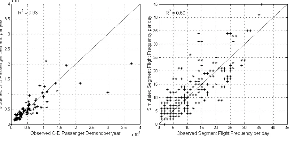
(ASM) in 2005 (OAG, 2005). Validation results, comparing modeled and observed O-D passenger
demand, city-pair flight frequencies, and flight segment frequencies, are presented in Figure 2. A
diagonal line is added in each chart, representing an exact match between the modeled results and
observed data. In order to quantify the proportion of variability in the observed data that is
explained by the model, an R-squared value is calculated across the network for each indicator.
These are also shown in Figure 2.
Figure 2a shows data points distributed approximately evenly along the diagonal line, although with
some outliers well below it. The latter can be attributed to unusual demand patterns, such as
between New York and Miami, which has uncharacteristically high vacation traffic. Mainly because
of these outliers, total system passenger demand is under-predicted by 8%. Figure 2b shows data
points distributed either side of the diagonal line, although with slightly more points above it than
below. This bias reflects an over-prediction of total segment flight frequency by 15%. The
R-squared values comparing the modeled and observed O-D passenger demand and segment flight
frequencies (0.63 and 0.60 respectively) seem acceptable for cross-sectional data.
9 New York City, Chicago, Atlanta, Washington, Los Angeles, Dallas/Fort Worth, Houston, San Francisco, Miami,
17
[image:18.612.73.540.68.300.2](a) (b)
Figure 2. Comparison of modeled results and observed data: (a) O-D demand, (b) segment flight
frequency.
If we compared modeled and observed city-pair (instead of airport pair) flight frequency, the
R-squared would increase from 0.60 in Figure 2b, to 0.80, as the degree of freedom from and to which
metropolitan airport to fly is removed. Therefore one of the primary contributors to the differences
in modeled and observed segment flight frequencies is the distribution of flights within
multi-airport systems. In fact, many of the outliers is Figure 2b include at least one multi-airport that forms part
of a multi-airport system. While the model distributes flights between airports in multi-airport
systems in such a way as to maximize airline profit (taking into account differences in operating
costs due to congestion and landing fees), it does not account for passenger choice, affected by e.g.,
airport accessibility. Such effects may be captured in future work through including passenger
18
4. Estimating the Magnitude of the Rebound Effect
The magnitude of the rebound effect within the above described U.S. aviation network was
estimated using the model described in Section 2 by simulating passenger and airline responses to
reduced aircraft fuel burn. For that purpose, fuel burn is reduced for all aircraft in the fleet in 5%
steps, up to a total reduction of 30%. The latter represents the expected fuel burn reduction of large
blended wing body aircraft (Greener by Design, 2005) and narrow body aircraft designed to operate
with advanced open rotor (ultra-high bypass ratio) engines (Lawrence et al., 2009) relative to conventional aircraft.10
The response of the air transport system to the hypothetical introduction of low fuel burn
technologies is compared to a base case in which no new technology is introduced. Input data,
including baseline aircraft performance data, fuel prices, airline operating costs, average fares, and
population and per capita income data (as described in Section 2), are applied for the year 2005.
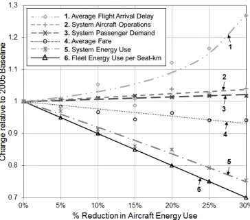
Figure 3 presents the simulation results for the modeled network of airports and cities in the United
States, relative to the 2005 baseline result. Relative changes in average fares, passenger demand,
aircraft operations, flight arrival delay (applying 2005 airport capacities), and system energy use are
plotted against percentage change in aircraft fleet energy use per seat-km. For reference, the relative
change in aircraft fleet energy use per seat-km is also plotted—a straight line with a gradient of -1.
10 Although reductions in fleet fuel burn would materialize gradually, the rate of fleet turnover would not affect the
magnitude of the rebound effect. The rebound effect could be affected by significantly higher capital costs of the new
aircraft technology that could reduce the cost savings. However, annualized capital costs are only a small percent of
total operating expenses (4%, on average, across U.S. major carriers in 2005) and thus even a drastic increase in capital
19
Because of the integer nature of the problem being solved at different percentage changes in aircraft
fleet energy use per seat-km, the plotted simulation results do not form a smooth curve. This is
typical for optimization results, and particularly for results of an integer program. In order to gain
insight into the general trends, curves are therefore fitted to the simulation results, from which the
system response is quantified. Reduced form equations are used to define these curves in order to be
consistent with theory. These equations, which are fitted using ordinary least squares, are described
[image:20.612.123.487.255.576.2]in detail in Appendix B.
Figure 3. Simulated changes in average system-wide flight arrival delay, aircraft operations,
passenger demand, airfare, and system energy use with reductions in aircraft fleet energy use per
20
Table 3 presents the average percentage change of each determinant of the rebound effect per
percent reduction in aircraft fleet energy use per seat-km and the associated R-squaredof the
[image:21.612.98.516.221.381.2]reduced form least-squared fits.
Table 3. Average change per percent reduction in aircraft fleet energy use per seat-km and
associated R-squaredof the reduced form least-squared fits.
% Change R2
Average Flight Arrival Delay (1) 0.49 0.896
Aircraft Operations (2) 0.12 0.872
Passenger Demand (3) 0.07 0.714
Average Fare (4) -0.23 0.769
System Energy Use (5) -0.81 0.986
Notes: Numbers in parenthesis relate to line numbers in Figure 3.
Passenger demand increases, on average, by 0.07% for every percent reduction in aircraft energy
use. This is partly a consequence of the decline in airfares, on average, by 0.23% for every percent
reduction in aircraft energy use, which comes with the introduction of low fuel burn technology in a
competitive market. (The decline in airfare is smaller than the reduction in fuel burn because fuel
burn is only one cost element incurred by airlines). Passenger demand and fares are also affected by
flight delays, which are driven by changes in aircraft operations, given available airport capacities.
While the reduction in airfare causes passenger demand to increase, flight delays affect passenger
demand negatively (as shown by the high passenger value of delay in equation 1). As passenger
21
reduction in aircraft energy use. This growth in aircraft operations occurs at a slightly faster rate
than the increase in passenger demand because the drop in operating costs allows for an increase in
frequency competition between competing airlines. The average simulated flight arrival delay
increases, on average, by 0.49% for every percent reduction in aircraft energy use, from 16.5
minutes in the base case (which compares to an observed value of 11.3 minutes in 2005) to 21.0
minutes at a 30% reduction in aircraft energy use. In a more constrained system this increase may
be significantly larger, as described in Section 5.
The studied flight network is not expected to change significantly with the assumed decrease in fuel
burn (the percentage of connecting passengers remains approximately constant at 8%). The
reductions in fuel burn are not large enough to drive significant changes in network routing.
Accordingly, average O-D passenger travel times (excluding flight delays) do not change
significantly either (remaining approximately constant at 3 hours 7 minutes). While projected
changes in network routing are small here, in other scenarios the same model has predicted
significantly larger adjustments, such as in a highly capacity constrained system (Evans and
Schäfer, 2011).
Jointly, the reduction in aircraft fleet energy use per seat-km and the adjustments described above
lead to a decline in system-wide energy use, which is also shown in Figure 3 and Table 3. The
resulting simulated decrease in system energy use is, on average, 0.81% for every percent reduction
in aircraft energy use, which corresponds to an average rebound effect of 19%. This gap can be
visualized by comparing curves 5 and 6 in Figure 3. The slightly convex curved shape of the system
energy use (curve 5) translates into a rebound effect that gradually decreases from 21% (for a 5%
22
rebound effect with continuous reductions in aircraft energy use can, in part, be attributed to a finite
aviation system capacity—the increasing travel demand is more and more counterbalanced by rising
flight delays. Irrespective of the exact decline in aircraft energy use, these estimates of the rebound
effect in the aviation sector are well within the range of the 10 to 30% estimate for automobile
travel identified by Greening et al. (2000).
5. Sensitivity of the Results
The rebound effect quantified above accounts for the passenger demand response to the
introduction of low fuel burn technology, the complementary airline operational effects, and
congestions effects. In order to identify the impact of airline operational effects and congestion
effects on the rebound effect, the simulation described above was rerun under different
assumptions.
In a first analysis, the model was rerun with a fixed flight network, fixed passenger load factors, and
a fixed distribution of aircraft sizes across the network. Flight frequencies for all aircraft size classes
are therefore scaled directly with changes in passenger demand. By eliminating airline operational
effects such as frequency competition, network optimization, and aircraft size choice, only
passenger demand and congestion effects are accounted for. Under such constraints, the simulated
system energy use declines, on average, by 0.84% for every percent reduction in aircraft energy use,
corresponding to an average rebound effect of 16%. This rebound effect is therefore 3 percentage
point lower than that derived with the full model and suggests that airline operational effects can
have a noticeable impact on the magnitude of the rebound effect, at least under the changes in
23
there is no increase in frequency competition between airlines, so aircraft operations increase less
strongly than in the case with the full model to accommodate the increase in demand.
A second sensitivity test quantifies the impact of airport congestion on the rebound effect, by
rerunning the full model with unconstrained airport capacities. In this case, system energy use only
declines at an average rate of 0.78% per percentage decrease in fuel burn, corresponding to an
average rebound effect of 22%. The resulting rebound effect is 3 percentage points greater than in
the case with existing airport capacities, which suggests that congestion effects may have a sensible
impact on the magnitude of the rebound effect. With no growth in flight delays associated with the
increases in aircraft operations, passenger demand increases, on average, by 0.13% for every
percent reduction in aircraft energy use – more strongly than in the case with airport capacity
constraints, consistent with the passenger value of delay estimated for equation 1. Because there are
no flight delays, operating costs decrease faster than in the case with airport capacity constraints,
resulting in simulated fares decreasing, on average, by 0.24% for every percent reduction in aircraft
energy use – slightly faster than in the case with airport capacity constraints. These results suggest
that, with an increase in airport congestion, the rebound effect is likely to decrease, possibly
significantly, because of the non-linear relationship between flight delays and airport capacity, and
the nonlinear cost of flight delay to airlines.
The sensitivity of the estimated rebound effect to the elasticity of passenger demand with respect to
generalized cost (τ in equation 1) was also examined. Increasing τ by one standard deviation (from
-0.60 to -0.73) leads to an increase in the rebound effect by 4.0 percentage points, and vice versa.
24
costs can be expected, as the demand response to changes in airfare (and travel time) is the ultimate
driver of the rebound effect
5. Conclusions
The analysis presented in this paper suggests that the average rebound effect in the studied network
within the domestic U.S. aviation sector is about 19%, for the range of aircraft fuel burn reductions
considered. This value is the net result of various effects. Most important is an increase in supply to
satisfy the rising air travel demand that comes with the introduction of more fuel-efficient aircraft.
This effect is supplemented by airline operational effects, most notably increasing frequency
competition, which increases the rebound effect by 3 percentage points. Finally, the mitigating
effect of delays due to traffic congestion decreases the rebound effect by 3 percentage points. These
latter results suggest that airline operational effects and congestion effects may both have a sensible,
although opposite, impact on the magnitude of the rebound effect. The estimated rebound effect
compares well to those for automobile travel. However, if the objective is to reduce greenhouse gas
emissions, the impact of a similar-sized rebound effect is more severe in aviation, given this
sector’s much more limited low-carbon fuel substitution opportunities, unless the rebound effect is
eliminated by taxes to keep airfares unchanged. Given that fuel accounted for about 32% of total
operating costs in 2005, a rebound effect in the order of 19% would require imposing a significant
fuel tax (equivalent) of 72%.11 Given a jet fuel price of 46 cents per liter in 2005 (ATA, 2008), the
tax would correspond to 33 cents per liter. This compares to a current fuel tax for domestic flights
within the U.S. of only 0.9 cents per liter (Schäfer et al., 2009). However, such a fuel price increase
25
could have dramatic economic consequences for an industry that operates at very small profit
margins.
While the estimated rebound effect applies to the studied subset of the domestic U.S. aviation
sector, it is likely to be significantly higher in the emerging markets of the developing world. Over
time, as income continues to grow, airfare elasticities decline, and the value of time increases, the
rebound effect is likely to decline. Along this reasoning, the rebound effect should also continue to
decline within the mature markets of the industrialized world, as has been observed for automobiles
(Small and Van Dender, 2007).
The analysis presented in this paper can only be a first step toward a better understanding of the
magnitude of the rebound effect in aviation. Perhaps most importantly, a more sophisticated study
would explicitly simulate fare competition on each individual route, leading to different rebound
effects on different routes. This approach may lead to a slightly lower system-wide rebound effect,
as decreases in operating costs may not be fully passed on to passengers on the less competitive
routes within an airline’s network. Albeit significantly more complex, such an analysis would be a
logical next step in this research.
References
ATA (Air Transport Association), 2008. Fuel 101: From Well to Wing. Document available online
at: http://www.airlines.org/economics/energy/fuel+101.htm [Accessed 8 February 2008].
Battersby, B., Oczkowski, E., 2001. An Econometric Analysis of the Demand for Domestic Air
26
Belobaba, P., 1989. Application of a Probabilistic Decision Model to Airline Seat Inventory
Control, Operations Research, Vol. 37, pp. 183-197.
Belobaba, P., 2006. Airline Economics Review, Course 16.75J / 1.234J Airline Management.
Massachusetts Institute of Technology, Cambridge, MA. Document available online at:
http://ocw.mit.edu/courses/aeronautics-and-astronautics/16-75j-airline-management-spring-2006/lecture-notes/lect2.pdf (Accessed 25 March 2011).
Belobaba, P., 2011. Personal communication.
Carrier, E., 2006. Modeling the Joint Choice of an Airline Itinerary and Fare Product: Implications
for Airline Pricing Strategies, Transportation Research Board 86th Annual Meeting, Washington,
DC, USA.
Corsi, T., Dresner, M., Windle, R., 1997. Air Passenger Forecasts: Principles and Practices. Journal
of the Transportation Research Forum, 30(2): 42-62.
DOT (United States Department of Transportation), Office of the Secretary of Transportation, 1997.
Departmental Guidance for the Valuation of Time in Economic Analysis. Document available online at: http://ostpxweb.dot.gov/policy/Data/VOT97guid.pdf (Accessed 10 September 2007).
DOT (U.S. Department of Transportation), 2005. Air Carrier Statistics and Financial Reports (Form
27
http://www.transtats.bts.gov/Tables.asp?DB_ID=135&DB_Name=Air%20Carrier%20Financial%2
0Reports%20%28Form%2041%20Financial%20Data%29&DB_Short_Name=Air%20Carrier%20F
inancial (Accessed 2 October 2012).
DOT (U.S. Department of Transportation), 2007. DB1B Survey. Document available online at
www.transtats.bts.gov (Accessed 10 September 2007).
DOT (United States Department of Transportation), Research and Innovative Technology
Administration, Bureau of Transportation Statistics, 2010. U.S. Air Carrier Traffic Statistics
Through December 2010. Document available online at:
http://www.bts.gov/xml/air_traffic/src/index.xml#CustomizeTable [Accessed 6 April, 2011].
Dray, L.M., Evans A.D., Reynolds T., Schäfer A., 2010. Mitigation of Aviation Emissions of
Carbon Dioxide, Transportation Research Record, 2177, pp. 17-26.
EUROCONTROL, 2004. Base of Aircraft Data (BADA), Version 3.6. Document available online
at: http://www.eurocontrol.int/eec/public/standard_page/proj_BADA.html [Accessed 15 July 2010].
Evans, A.D., 2008. Rapid Modeling of Airport Delay. 12th Air Transport Research Society World
Conference, Athens, 6-9 July.
Evans, A.D., 2010. Simulating Airline Operational Responses to Environmental Constraints. Ph.D.
Dissertation, University of Cambridge. Document available online at:
28
Evans, A., Schäfer, A., 2011. The impact of airport capacity constraints on future growth in the U.S.
air transportation system. Journal of Air Transport Management (2011),
doi:10.1016/j.jairtraman.2011.03.004.
Forbes, S.J., 2008. The effect of air traffic delays on airline prices. International Journal of
Industrial Organization, 26(2008): 1218–1232.
Fudenberg, D., Tirole, J., 1991. Game Theory, MIT Press, Cambridge MA
Greene, D.L., Kahn, J.R., Gibson, R.C., 1999. Fuel Economy Rebound Effect for U.S. Household
Vehicles. The Energy Journal, 20(3): 1-32.
Greening, L.A., Greene, D.L., Defiglio, C., 2000. Energy Efficiency and Consumption – the
Rebound Effect – a Survey. Energy Policy, 28(6-7): 389-401.
Greener by Design Science and Technology Sub-Group, Royal Aeronautical Society, 2005. Air
Travel – Greener by Design, Mitigating the Environmental Impact of Aviation; Opportunities and
Priorities.
IATA (International Air Transport Association), 2008. Airport and Air Navigation Charges Manual.
29
ICAO (International Civil Aviation Organization), 2007. ICAO Aircraft Engine Emissions
Databank. Document available online at:
http://www.caa.co.uk/default.aspx?catid=702&pagetype=90 [Accessed 10 June 2008].
Jamin, S., Schäfer, A., Ben-Akiva, M.E., Waitz, I.A., 2004. Aviation Emissions and Abatement
Policies in the United States: A City Pair Analysis. Transportation Research Part D, 9(4): 294-314.
Kostiuk, P.K., Gaier, E., Long, D., 1998. The Economic Impacts of Air Traffic Congestion,
Logistics Management Institute, McLean, VA, IR811S1. Document available online at
http://www.boeing.com/commercial/caft/reference/documents/lmi_econ.pdf (Accessed 29
December, 2012).
Khazzoom, D.J., 1980. Economic Implications of Mandated Efficiency Standards for Household
Appliances. Energy Journal (1): 21–40.
Lawrence, J., Kingan, M., Self, R., 2009. Integrated Study of Advanced Open Rotor Powered
Aircraft, Omega Study No. 8, Final Report for the Omega Consortium. Document available online
at:
http://www.omega.mmu.ac.uk/Events/Study%208%20Report%20Revised%20FORMATTED-%20300309.pdf [Accessed 9 October, 2009].
Morrison, S.A., Winston, C., 1989. Enhancing the Performance of the Deregulated Air
30
Mumayiz, S.A., Pulling, R.W., 1992. Forecasting Air Passenger Demand in Multi-Airport
Regions”, Proceedings of the Transportation Research Forum. 34th (1992), V. 1, 31, Arlington, VA.
Nash, J.F., 1950. “Equilibrium points in n-person games”, Proceedings of the National Academy of
the USA 36 (1): 48–49, doi:10.1073/pnas.36.1.48, PMC 10688946
OAG (Official Airline Guide), 2005. “OAG 2005 Flight Schedule Database”, OAG
Worldwide Inc.
Pulles, J.W., et al., 2002. Aviation Emissions and Evaluation of Reduction Options (AERO) Main Report, Director General for Civil Aviation, Ministry of Transport, Public Works and Water
Management of the Kingdom of the Netherlands.
Reynolds, T., Barrett, S., Dray, L., Evans, A., Köhler, M., Vera-Morales, M., Schäfer, A., Wadud,
Z., Britter, R., Hallam, H., Hunsley, R., 2007. Modeling Environmental & Economic Impacts of
Aviation: Introducing the Aviation Integrated Modeling Tool. 7th AIAA Aviation Technology,
Integration and Operations Conference, Belfast, 18-20 September.
Schäfer, A., Heywood, J.B., Jacoby, H.D. & Waitz, I.A., 2009. Transportation in a
Climate-Constrained World. Cambridge (MA): The MIT Press.
Meyer, J.R., et al., 1999. Entry and Competition in the U.S. Airline Industry: Issues and Opportunities, Special Report 255, Transportation Research Board, National Research Council,
31
U.S. Census Bureau, 2000. Census 2000. Document available online at:
http://www.census.gov/main/www/cen2000.html [Accessed 10 September 2007].
Small, K., Van Dender, K., 2007. Fuel Efficiency and Motor Vehicle Travel: The Declining
Rebound Effect, Energy Journal 28(1): 25-51.
U.S. Census Bureau (2005). American Community Survey 2005. Document available online at: http://www.census.gov/acs/www/ [Accessed 10 September 2007].
Waitz, I., et al., 2006. Prototype Work Plan for the Aviation Environment Portfolio Management Tool, Partnership for AiR Transportation Noise and Emissions Reduction (PARTNER), Report No.
PARTNER-COE-2006-003.
Wingrove, E.R., E.M. Gaier, T.E. Santmire, 1998. The ASAC Air Carrier Investment Model (Third
32
Appendix A
The Travel Time Calculator calculates segment flight times as a function of unimpeded
(delay-free) flight time by aircraft type (calculated using BADA (EUROCONTROL, 2004) and the
Aircraft Engine Emissions Databank (ICAO, 2007)). Average passenger O-D travel times are
calculated for all city-pair passenger itineraries based upon the travel times for each flight segment.
Only non-stop itineraries and itineraries with a single connection are considered. The Delay
Calculator, described in detail by Evans (2008), models the impact of airport capacity constraints
on airline costs and passenger travel times. In this model, flight delays, both on the ground and in
the air, are estimated as a function of flight frequencies and airport capacity using queuing theory,
and are added to gate departure delays due to mechanical failures and late arrivals (assumed to
remain at current levels due to more widespread schedule padding to maintain schedule reliability).
Runway departure delays are distributed between the taxiway and gate according to a taxi-out
threshold calculated for each airport from historical delay data. Similarly, delays due to destination
airport capacity constraints are distributed between the air and ground according to an airborne
holding threshold calculated for each airport from historical delay data, and above which delay is
33
Appendix B
Reduced form equations are used to define the curves in Figure 3 in order to be consistent with
theory. These equations, which are fitted using ordinary least squares, are described below.
Because fares are scaled with operating costs, which directly depend on aircraft fuel use, they
decrease linearly with declining aircraft energy use. Based on equation (1), and assuming that flight
frequency is a linear function of passenger demand (only strictly true when airline operational
effects and airport congestion effects are not modeled, which is not the case here), changes in
passenger demand take the following form, as a function of relative reduction in aircraft fleet
energy use per seat-km:
(3)
where D/D0 is the ratio of simulated and baseline passenger demand, C1 is a constant, (E0-E)/E0 is
the relative reduction in aircraft energy use, τ is the elasticity of the generalized cost term in
equation (1), and β is the elasticity of flight frequency in equation (1). Flight frequency takes the
same form, given the assumption that flight frequency is a linear function of passenger demand. A
curve of this form is therefore fitted to the passenger demand and the flight frequency data in Figure
3. Given that airport congestion is modeled by an M/M/1 queuing system, with server demand
defined by flight frequency, changes in average flight delay take the following form, as a function
of the relative reduction in aircraft energy use:
(4)
! !! = !!∙
!!−!
!! +1
!
!!!
!"#$% !"#$%! = 1−!! 1−!! !!∙
!!−! !! +1
34
where Delay/Delay0is the ratio of simulated and baseline average flight delay, C2 is a constant, and (E0-E)/E0, C1, τ and β are as defined for equation (3). Assuming that system energy use is directly
proportional to flight frequency (only strictly true when changes in aircraft size and congestion
effects are not modeled), changes in system energy use takes the following form, as a function of
the relative reduction in aircraft energy use:
(5)
where ESYS/ESYS 0 is the ratio of simulated and baseline system energy use, and (E0-E)/E0, C1, τ and β
are as defined for equation (3).
!!"! !!"!!! = 1−
!!−!
!! !!∙
!!−!
!! +1
!