Multi-scale quantification of leaching performance using X-ray tomography

Multi-scale quanti

fi

cation of leaching performance using

X-ray tomography

Q. Lin

, S.J. Neethling

⁎

, L. Courtois

, K.J. Dobson

, P.D. Lee

Rio Tinto Centre for Advanced Mineral Recovery, Department of Earth Science and Engineering, Imperial College London, London SW7 2AZ, United Kingdom b

Manchester X-ray Imaging Facility, School of Materials, University of Manchester, Oxford Rd., M13 9PL, United Kingdom c

Research Complex at Harwell, Rutherford Appleton Laboratories, Harwell, Didcot, Oxfordshire OX11 0FA, United Kingdom

a b s t r a c t

a r t i c l e i n f o

Article history:

Received 26 February 2016 Received in revised form 28 May 2016 Accepted 23 June 2016

Available online 25 June 2016

The performance of heap leaching is dictated by a large number of processes acting at a wide range of length scales. One important scale is that of the individual particles, where the interaction between the rate kinetics at the surfaces of the individual mineral grains and the mass transport through the particle combine to give the overall apparent particle scale kinetics. It has been recognised for a long time that variability in the mineral-ogy, size and spatial distribution of the mineral grains within the particle are likely to have a large effect on the leach performance and its variability and thus, ultimately, the performance of the heap. In this paper a new meth-od for quantifying this behaviour and its variability at scales from the particle through to the grain and down to the surface kinetics is presented. This method is based on the use of a series of XMT (also called micro-CT) images of a column taken at regular intervals over 168 days of leaching. The key development in the analysis of this data is an algorithm that has allowed every single one of the hundreds of thousands of mineral grains within the col-umn to be individually tracked across all the time points as they undergo dissolution. This has allowed the depen-dency of the mineral grain leach rate on its size and position in the particle to be decoupled from one another. It also meant that the variability in the surface kinetics of the grains could be assessed, with mineralogical variabil-ity being the key source of this variabilvariabil-ity. We demonstrate that understanding and quantifying this underlying kinetic variability is important as it has a major impact on the time evolution of the average kinetics of the leaching.

© 2016 The Authors. Published by Elsevier B.V. This is an open access article under the CC BY license (http://creativecommons.org/licenses/by/4.0/). Keywords:

Heap leaching Multi-scale Micro-CT Imaging Leaching variability

1. Introduction

While metal production has kept pace with increased demand this has generally been achieved by exploiting deposits with more problem-atic mineralogies and ever lower ore grades. As the grades of ores de-crease, heap leaching is becoming a more attractive alternative to conventional processing routes, such asflotation followed by smelting, as it does not require milling of the ore and the operating cost per unit of metal is thus less sensitive to grade. Approximately 20% to 30% of the world's copper and more than 12% of gold is produced by this tech-nique (Bouffard and West-Sells, 2009; Jergensen, 1999; Kappes, 2005). The biggest disadvantages of heap leaching, though, are the long pro-cessing time and relatively low extraction efficiencies, especially for pri-mary sulphides.

Research into heap leaching can be divided into a range of spatial scales involving different processes and sub-processes, including the

macro-scale (heap scale effects), meso-scale (groups of particles, typi-cally investigated through column scale studies), individual ore particle scale and grain scale (Dixon and Petersen, 2003). At each scale, there are several different sub-processes and control parameters which can affect leach behaviour. In general, conditions and concentrations in the_fluids around the ore particle, the mass (and heat) transport within the ore particle and surface reaction kinetics are the main factors which can af-fect the leach performance at the meso-scale and which determine the apparent leach kinetics. Most studies of heap leaching have either con-centrated on thefirst or last of these factors, either using particle sizes representative of real heaps and studying the apparent kinetics as a function of the effluent and/or feed conditions (e.g.van Hille et al. (2010)) at column or larger scale, or have attempted to obtain the sur-face reaction kinetics by studying the dissolution offinely milled ore or pure mineral particles in stirred tank experiments (Córdoba et al., 2008; Hiroyoshi et al., 2001) at the grain scale. A lack of data on the transport processes within the ore particles makes it very hard to predict heap or even particle scale leach performance based directly on the surface reac-tion kinetics, while only studying the behaviour based on the overall performance makes it hard to determine the dominant mechanisms at

Hydrometallurgy 164 (2016) 265–277

⁎ Corresponding author at: Department of Earth Science and Engineering, Royal School of Mines, Imperial College London, SW7 2BP, United Kingdom.

E-mail address:[email protected](S.J. Neethling).

http://dx.doi.org/10.1016/j.hydromet.2016.06.020

0304-386X/© 2016 The Authors. Published by Elsevier B.V. This is an open access article under the CC BY license (http://creativecommons.org/licenses/by/4.0/).

Contents lists available atScienceDirect

Hydrometallurgy

ferences in X-ray attenuation, which, in turn, depends on the electron density and hence a combination of the density and atomic mass of the materials. This means that within the copper ore used in this study the sulphide species can be readily distinguished from the mainly silicate gangue, though the various sulphide species have similar atten-uations and are thus hard to distinguish from one another.

In this work XMT has allowed 3D images of the mineral grain distri-butions to be obtained within the same leaching particles at a succes-sion of time points. In order to analyse this data we have developed advanced image quantification algorithms (Lin et al., 2015) that have allowed us to track the dissolution of many hundreds of thousands of in-dividual mineral grains over the course of many months of leaching. The analysis of this data set is thus the main focus of this paper. It should be noted that due to the difficulty in distinguishing different sulphide phases this paper examines the dissolution of the sulphide grains rather than specifically the copper extraction. In later sections where the grain scale variability is quantified, much of this will therefore come from mineralogical variability.

2. Experimental methodology

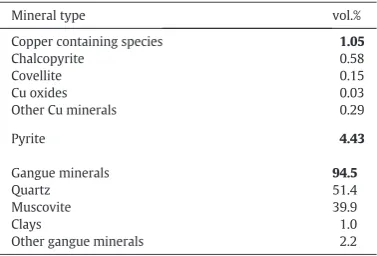
The leached sample consisted of copper sulphide ore particles from Kennecott with a size ranging between 8 and 11.2 mm. The ore compo-sition was obtained using the Mineral Liberation Analyser (MLA) (see Table 1).

As this method is destructive, the composition is not that of the actu-al particles in the column, but rather that of similar particles.

The small scale column leaching experiments were carried out using an incubator with temperature control, which allows multiple columns to be run at the same time. The reason for using an incubator is because, despite the exothermic reactions, small columns lose too much heat to

main leaching agent. This was done to mimic the effect of bacterial ac-tion, which in an actual heap would generate ferric ions mainly through a combination of the leaching of the pyrite and the oxidation of the fer-rous ions in solution. While there is still some controversy as to the exact mechanisms involved, especially for chalcopyrite, the overall fer-ric leaching reactions for the chalcopyrite and pyrite are typically de-scribed as being as follows, with a subsequent reaction in which a portion of the elemental sulphur is converted to a sulphate (Habashi, 1999):

CuFeS2þ4Fe3þ→Cu2þþ5Fe2þþ2S0 FeS2þ2Fe3þ→3Fe2þþ2S0 2S0_þ3O

2þ2H2O→4Hþþ2SO24−

3. Image acquisition and processing methodology

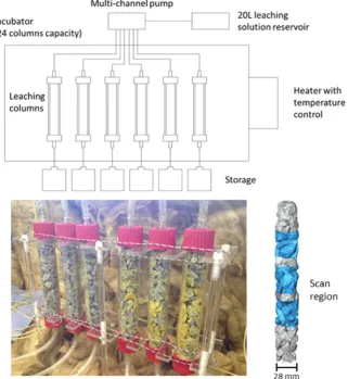
The columns used in this study were scanned using a Nikon Metris Custom Bay with a 1 mm aluminiumfilter (to reduce beam hardening effects), 89 kV energy, 0.708 s exposure time and 2001 projections. The detector size was 2000 × 2000 pixels, which gave a linear resolution of approximately 17μm. Three volumes (top, middle and bottom for each column) were scanned at each time point over the leaching period. Scanning was done by removing the entire column from the incubator and placing it within the scanner before replacing it within the incuba-tor. This was done as rapidly as possible in order to minimise the distur-bance to the column. As the leaching rate in the columns decreased with time, the interval between scans was increased. The scanning intervals are given inTable 2.

While the entire column was initially imaged, in subsequent scans the same three sub-volumes of the column were imaged (seeFig. 1). The reason for doing this was a combination of the most efficient use of the available equipment time, as well as the desire to minimise dis-ruption of the feed and heating of the column. The total number of tracked whole ore particles1within these three sub-volumes was 26 for this column.

After scanning, the images needed to be reconstructed and relevant data quantified. The main image processing steps were as follows:

1. The reconstructed image had a 3 × 3 × 3 medianfilter applied to re-duce the noise level.

2. The rock phase was thresholded using the Otsu algorithm (Otsu, 1979). This algorithm was used as there are distinct peaks in the in-tensity histogram between the rock and the air phases.

Table 1

Main mineral species within ore sample used in experiments. Prev-alence is reported as volume percentages as these are most relevant to micro-CT analysis, which also measures volume.

Mineral type vol.% Copper containing species 1.05

Chalcopyrite 0.58

Covellite 0.15

Cu oxides 0.03

Other Cu minerals 0.29

Pyrite 4.43

Gangue minerals 94.5

Quartz 51.4

Muscovite 39.9

Clays 1.0

Other gangue minerals 2.2

1

3. The connected ore particles were separated using a distance transfor-mation based method with marker control to avoid over segmentation.

4. Each ore particle was then labelled and tracked over the leaching pe-riod using a centroid tracking algorithm (Blair and Dufresne, 2008). This was required both because the ore particles settle and rotate over the course of the leaching and because the orientation of the col-umn varies slightly between scans.

5. After extracting the same ore particle from different scans, the initial ore particle was registered according to the later scan in order to have the same orientation at each time point. The extracted 4 × 4 transformation matrix is a key input into the grain tracking algorithm.

6. The mineral grain phase was then thresholded using the Maximum Entropy algorithm (Kapur et al., 1985). The reason for using this algo-rithm is that the relatively small quantity of sulphide in the ore means that it does not exhibit a distinct peak in the intensity histogram.

7. All the mineral grains in the scanned volume were then tracked indi-vidually using a new fast tracking method. A detailed description of the grain tracking methodology can be found inLin et al. (2015). Fig. 2a) and b) show a slice through a particle before leaching and after 168 days of leaching in which all the grains have been correctly

matched to their corresponding grains in the earlier image despite some of the grains disappearing completely or splitting into multiple segments.Fig. 2c) shows the tracking of a single large grain over the course of the experiment.

4. Investigation of leach performance and variability

In this section the leach behaviour and its variability at different scales are investigated. The average sulphide dissolution for the entire column, the average sulphide dissolution for the three scanning regions and the sulphide dissolution for all the tracked ore particles can be mea-sured from the image analysis (Fig. 3), each showing different levels of variability.

4.1. Leach performance and variability at the particle scale

The vertical leach variability is small, with no discernible trend in the extraction with height (Fig. 4d). This is due to the scale of the column and the narrowly sized ore particles. The horizontal leach variability can also be measured by considering the location of the ore particles, which is characterised by the distance between the centroid of each par-ticle and the centre of the column (Fig. 5). As the column is very narrow (internal diameter of the column was 28 mm), theflow can spread Fig. 1.Schematic diagram of small scale column leaching experiment and columnsfilled with ore particles and the scanning regions.

Table 2

XMT scanning intervals for the small scale leaching columns. Scanning points (end of leaching day)

0 1 5 11 16 23 33 43 53 83 118 136 168

267

relatively evenly and there is no discernible trend in the extraction with horizontal position in the column (reflected by the weak linear correla-tion coefficient (r) and coefficient of determination (r2_)).

The lack of variation in extraction with height in the column or with horizontal position means that the variability between particles is virtu-ally all due to local effects such as differences in the mineralogy of the particles and the spatial and size distribution of the grains within then. The ore particle size effect is known to be an important mechanism affecting the sulphide dissolution (Ghorbani et al., 2011a), but the inves-tigation of this dependency was not the aim of these experiments and a

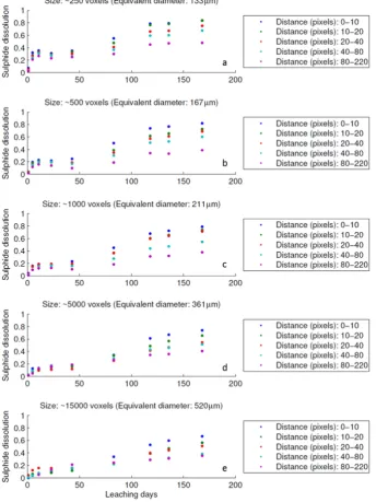
narrow size distribution for the particles was deliberately chosen to try and limit this effect.Fig. 6shows the sulphide dissolution against the initial ore particle size for all the tracked particles within the column. The total volume (in voxels) of each particle was measured using the voxel counting algorithm and converted into an equivalent spherical diameter (in mm). The narrow size distribution means that the particle to particle variability masks any underlying trend in extraction with size. The three main sources of leach variability within the particles are likely to come from the size distribution of the grains, the variability in the inherent surface kinetics (mainly a function of mineralogy and min-eral associations) and the distribution of the distances of the grains to the ore particle surface (which will impact the mass transfer rate). The mineral grain distance distribution can be measured and quantified by applying a 3D distance map. In the distance map analysis, each voxel is assigned a value depending on the distance to the nearest ore particle boundary. The boundary voxels of the object are assigned a value of zero whereas the assigned value increases as the distance from the boundary increases. Generally, the mineral grains closer to surface should leach faster than the minerals located in the centre of ore particle. This is be-cause the shorter the distance to the surface, the easier it is for the leaching solution to diffuse in and the dissolved species to diffuse out. Fig. 7shows a distance plot of an example particle over 168 days of leaching. A strong distance dependency can be observed.

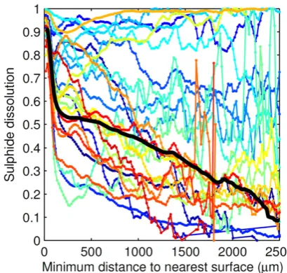
Among all 26 particles, the majority have similar trends to that shown inFig. 7, though there is still quite a bit of variability brought about by differences in the size and spatial distribution of the grains, as well as in their mineralogy. While there is likely to be little correlation on average, within individual particles grain size can be correlated with distance to the particle surface. In particular, the location and leach be-haviour of a few large grains can have a disproportionate impact on these curves for an individual ore particle.Fig. 8shows the average ex-traction with distance over all 26 of the measured particles after Fig. 2.Examples showing mineral grain tracking. a–b) An example slice of mineral grains within an ore particle after leaching. Different colours indicate individual mineral grains. c) Mineral grain tracking for an example grain over 168 leaching days.

168 days of leaching, as well as the extraction against distance curves for all 26 individual particles. To better understand these trends we need to decouple the effect of distance from that of particle size, though

fortunately the ability to track the leach behaviour of every single min-eral grain means that we have a vast amount of data with which to do this (136,443 individual grains were tracked within the 26 particles). Fig. 4.The initial conditions of scanned volumes and their overall sulphide dissolution. The error bars indicate the uncertainty caused by the thresholding algorithm, which is ±2%. The resolution of the scanning is approximately 17μm. The value of ±2% is measured by comparing the total volume of tracked mineral grains for a rescanned volume to its reference volume (details shown in (Lin et al., 2015)). This error value is suitable for measuring the total volume of mineral grains with a wide size distribution rather than grains at a specific size.

Fig. 5.The sulphide dissolution for all the tracked ore particles against the distance between the centroid of the ore particle and the centre of the column (pixels).

Fig. 6.The sulphide dissolution for all the tracked ore particles against their initial ore particle sizes.

269

4.2. Leach performance and its variability at the mineral grain scale

The mineral extraction is a strong function of its distance to the ore particle surface (seeFig. 8), though with quite a bit of variability be-tween particles. Much of this leach variability is likely to be due to var-iability in the distributions of size and distance to the particle surface of the individual mineral grains. In order to fully understand the leach per-formance and its variability, and to determine the dominant mecha-nisms, the analysis thus needs to be carried out at the grain scale.

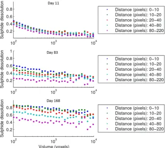
Analysing tens of thousands of grains individually is not very mean-ingful or efficient, especially for smaller grains, which have high mea-surement errors and uncertainties when considered on their own. Combining the measurements from many similar grains will, however, significantly reduce this uncertainty (Lin et al., 2015). Therefore, it is more useful to divide all the grains into different size–distance catego-ries and study the average leach behaviour and its variability for each category. The grains were divided into categories based on size and dis-tance to the surface with intervals chosen to give a reasonable distribu-tion of the grains over the categories (seeFig. 9). Without having different size intervals for different distance categories it is impossible to perfectly balance the number of grains in each category. As they have smaller measurement errors associated with them, it is less

important to have a large number of grains in the categories with larger grain sizes (Lin et al., 2015).

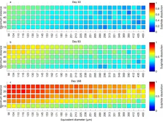
The average sulphide dissolution for different size–distance catego-ries is shown inFig. 10. The categories shown are those with an average size larger than 100 voxels and a sample size larger than 10. A clear col-our gradient can be observed with increasing average initial grain size and average distance to the ore surface. The colour gradient indicates that the grains with smaller size and shorter distance have higher leaching kinetics, as expected.

While it is obvious that the leach rate of a grain should depend upon its distance from the surface and its size, it is interesting to investigate the relative importance of these dependencies and how they vary with time. FromFig. 11it can be seen that in all size and distance cate-gories there is an initial rapid jump in the sulphide dissolution over the

first few days of leaching. This is probably due to the small amount of oxides and secondary sulphides within the system (see.Table 1), which are known to have much faster leach kinetics than the primary sulphides.

FromFigs. 11 and 12it can be seen that the size dependency is the dominant effect at short times, while the distance dependency becomes stronger at longer times. This change in relative importance of size and distance is probably not due to any change in the mechanisms involved, but is rather due to variability in the leach rates of the individual grains within a size and distance category. The extraction is being characterised by means of the initial size of the grains, which means that as time progresses the variability of the current size of the grains within a category becomes wider and thus the dependency on the initial size becomes weaker. The variability in the leach rate of grains within a size and distance category is likely to be mainly due to variability in the surface kinetics and thus a function of the variability in the mineralogy and its associations. It is thus important to investigate this variability in the leach rate within each category as it will have a major bearing on the apparent leach kinetics and their evolution with time.

Within a single ore particle,Fig. 13shows the change in sulphide dis-solution for 25 mineral grains chosen randomly out of those that have an initial volume of between 500 and 1000 voxels (this corresponds to initial equivalent spherical diameters of between about 75μm and 95μm). As well as these 25 randomly chosen grains, the average behav-iour of all 394 mineral grains within this category is plotted. While the uncertainty in the size of the individual grains due to measurement error within this size range is small, it is not trivial (a relative standard deviation of about 3% to 4%), the effect of measurement error on the cal-culation of the average leach behaviour is tiny, though, due to the large Fig. 7.Distance plot for an example ore particle over the 168 day leaching period.

Fig. 8.Average sulphide dissolution for all tracked ore particles versus the distance between each grain and nearest surface over 168 leaching days.

sample size (seeLin et al. (2015)for details on how the measurement uncertainty is obtained). The measurement uncertainty will be the rea-son why a small number of the recoveries for individual mineral grains are below zero, especially as these values are particularly sensitive to er-rors in the measured volume of the grains in the initial scan as this infl u-ences every subsequent dissolution value.

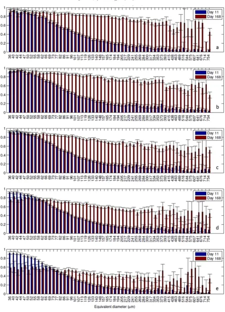
Our error analysis has shown that for all but the smallest grains (those below about 100 voxels (equivalent spherical diameter of ~98μm with pixel size of 17μm) the variability in the measured extrac-tion is primarily due to variability in the actual underlying leach rate rather than measurement error. The error bars inFig. 14thus represent differences in the actual leach rate of grains, which have similar initial sizes and distances to the surface. This variability is likely to come from differences in the mineralogy of the grains themselves, as well as due to different mineral associations and local differences in the perme-ability of the rock surrounding the grains.

This variability in leach rate initially causes the variability in extrac-tion to increase with time, but as the number of completely leached grains increases, the variability in the extraction starts to decrease again as, irrespective of the variability in the rate at which they are leached, fully leached grains have no variability in their extraction.

It is desirable to go a step further than simply looking at the variabil-ity in the extraction to look at the underlying grain scale variabilvariabil-ity in the leach kinetics as this can be used to estimate how the apparent leach kinetics are likely to vary with time and the macroscopic extent of extraction.

5. Estimating variability in the surface kinetics

The variability in the surface kinetics is an important factor in the ul-timate performance of a heap as it controls how the apparent kinetics will evolve with time. Since grains with high leach kinetics will disap-pear faster than those with slow surface kinetics, the average surface ki-netics will decrease with time. Additionally, the faster leaching classes such as grains near the particle surface or smaller grains will also disap-pear faster. The evolution of the apparent leach kinetics of a particle is thus the result of a complex interaction between the evolution of the surface rate kinetic distribution, the size and location distribution of

the grains and how these interact with mass transport within the parti-cle. Accounting for all these factors is complex and can only really be assessed using a fully coupled modelling and simulation approach (e.g.Lin et al. (2016)). In this section of the paper we will concentrate on assessing the distribution of apparent surface rate kinetics and how this impacts the evolution of the mineral grain size distribution.

In order to assess the distribution of the surface rate kinetics we need to be able to use the extraction of the individual grains to calculate their rate kinetics. To do this we start with a very generic rate equation for surface kinetics. In the derivation below we have made no assump-tion about the order of the reacassump-tion (in fact, for the purposes of this der-ivation we need not even assume that there is a power law dependency):

F¼kCn ð1Þ

whereFis the mass_flux out of the grain,kis the surface rate constant andnis the order of the reaction. In this derivationCis the time depen-dent concentration experienced by grains within a particular category. The rate of change in the mass of a grain is equal to theflux out of the grain times its surface area:

dM dt ¼−kAC

n _ð2Þ

whereMis the mass of the grain,A is the surface area. The surface area of a grain is proportional to its volume raised to a power 2/3, with a pro-portionality,α, that depends on its shape:

A¼αV2=3 ð3Þ

The mass of the grain is, in turn, related to its volume by its density, ρ:

M_¼ρV _ð4_Þ

Fig. 10.Plots of average sulphide dissolution in each size–distance category in three difference time points using a colour map based on percentage dissolution: a) Day 33 b) Day 83 c) Day 186.

271

Combining these equations gives the following differential equation for the rate of change of grain volume:

dV dt ¼−

α ρkV

2=3

Cn ð5Þ

Eq.(5)can be integrated from the initial time to any subsequent time over which the grain volume changes from an initial volume,V0, to the volume at timet,Vt:

ZVt

V0 ρ

aV2=3dV¼−k Zt

0

Cndt ð6Þ

1 3 V0

1=3

−Vt1=3

¼α_ρk Zt

0

Cndt ð7Þ

We can do the same analysis for the grain in the same size and dis-tance category with the average surface rate,k, for that category and a corresponding average volume after timetofVt:

1 3 V0

1=3

−Vt

1=3

¼α_ρk Zt

0

Cndt ð8Þ

Dividing Eq.(7)by Eq.(8)removes all the dependencies other than that on the change in volume:

k k¼

1− Vt

V0 1=3

1− Vt

V0 1=3

ð9Þ

This equation can also be written out in terms of the extraction from a grain_ðR_¼1₋Vt

V0Þ:

k k¼

1−ð1−RÞ1=3

1−1−R1=3

ð10Þ

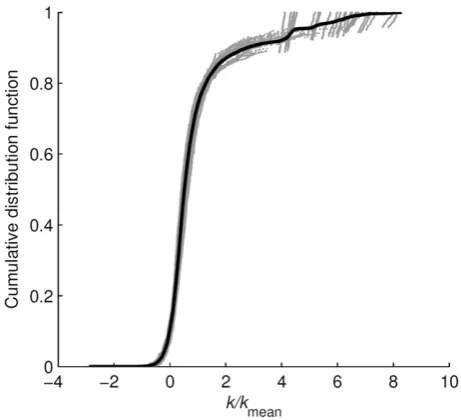
This analysis gives the surface rate constant of a grain relative to the average rate constant within a category and thus, by combining all the grains within a category, it can give the distribution of the apparent sur-face kinetics. In the analysis below, the distributions are calculated by using the sulphide dissolution of the all the measured mineral grains over thefirst 23 days of leaching.

Fig. 15shows the cumulative distribution of the relative rate con-stants for all the size and distance categories (i.e. based on all 136,443 grains). Even though the average leaching rates of the different catego-ries were markedly different (seeFig. 10), the distributions of the rela-tive rates are all remarkably similar.2_{This implies that this variability}

is predominantly a property of the mineral surfaces, local mineral

associations and local mass transfer barriers, since more macroscopic variability effects would manifest themselves as changes in the shape of this distribution with distance from the mineral surface.

InFig. 16the average over all the distributions is plotted as a proba-bility density function (PDF). This distribution has a major peak that is likely to be associated with the primary sulphides as these are both the slowest leaching and most abundant of the metal containing min-erals. There is also evidence for smaller peaks in this distribution at much higher leaching rates. These peaks are most likely associated with oxides and secondary sulphides that are known to have much faster leach kinetics (Bartlett, 1998).

2

In these distributions a few grains have negative apparent rates. This is probably be-cause of measurement uncertainty in the change in volume for grains with little or no leach kinetics. The upward spikes to 1 in the distributions for some of the faster leaching categories are due to the time interval over which the analysis was conducted. In some of the fastest leaching categories a number of grains will be completely leached within the 23 day time interval used to produce this data, putting a limit on the maximum relative rate that can be measured.

Fig. 12.The extent of dissolution (recovery) for different categories at different distance against average initial mineral grain size at different time points: e.g. Day 11, Day 83 and Day 168.

Fig. 13.The change in extent of dissolution (recovery) of 25 example grains with initial volumes of between 500 and 1000 voxels over the 168 days of leaching. In addition, the average dissolution behaviour for all 394 grains within this category is also plotted.

273

This underlying variability in the apparent surface leach kinetics together with the size and spatial distribution of the grains are key to the time evolution of the particle scale leach

kinetics. In a related paper (Lin et al., 2016) a methodology for incorporating this data into a detailed particle scale simulation is presented.

Fig. 14.The sulphide dissolution for all the size–distance categories with average initial grain size (equivalent spherical diameter) larger than 36μm after Day 11 and Day 168. a) Distance 0–0.17 mm (0–10 pixels). b) Distance 0.17–0.34 mm (10–20 pixels). c) Distance 0.34–0.68 mm (20–40 pixels). d) Distance 0.68–1.36 mm (40–80 pixels). e) Distance 1.36–3.74 mm (80–

5.1. Calculating the evolution of the grain size distribution

The distribution of the surface kinetics (Fig. 16) can be used to calcu-late the distribution of the extractions for the grains within a category given an average extraction for the category. This is, in effect, the reverse of the procedure used to calculate the distribution in thefirst place, though it can be used for any average extraction, not just the measured ones.

The extraction within a size and distance category is a function time, though not a known function for an arbitrary category. The extraction for the grain with the average surface kinetics can thus be written as a function of a time dependent variable,T, with the form being chosen to make the subsequent analysis easier (note that the average extrac-tion and the extracextrac-tion for the grain with the average surface kinetics is not the same thing as the extraction rate for a grain is also

proportional to its surface area, the distribution of which changes with time):

T¼f tð Þ ¼1−1−R1=3 ð11Þ

By combining Eqs.(10) and (11)and rearranging the following equation for the extraction of a grain with a specific relative rate con-stant,k

k, is obtained. The reason for the inequalities in this equation is

that extraction for a particular grain cannot be greater than 1.

R_¼

1− 1−Tk k

3

; 1− 1−Tk k

3

≤1

1; 1− 1−Tk k 3 N1 8 > > > < > > > :

ð12_Þ

IfVinitialis the probability density function (Fig. 16) for the initial vol-ume of grains with a relative surface rate constant k=k (where

∫

∞

0 Vinitialdð

k

kÞ ¼1), then the average extraction within a category after a

specific time,Rave, can be calculated:

Rave¼1−

Z∞

0

Vinitialð1−RÞd k

k ð13Þ

whereRis a function ofk

k(andT) as calculated from Eq.(12). Eq.(13)is

complex to solve analytically for an arbitrary probability density func-tion. In this paper this equation is solved numerically using the follow-ing approximation:

Rave≈1−

XN

i¼0

Vinitial;ið1−RiÞΔ k

k i ð

14Þ

whereiis an interval in the value ofk

kin the discrete version of the

prob-ability density function. This means that the distribution of recoveries (or, equivalently, sizes relative to the initial size) can be calculated as a function of the average extraction (seeFig. 17).3_{In this calculation a}

value ofTis chosen to given the desired value for the average extraction in a category by using Eq.(14)combined with an appropriate rootfi nd-ing algorithm (e.g. the“solve”function in Excel). As part of the calcula-tion of Eq.(14), all the individual recoveries are calculated using Eq. (12).

It should be noted that this is not a calculation for the evolution of the grain size distribution within an overall ore particle, but is rather a calculation of the evolution of the grain size distribution for grains at a similar distance to the surface and similar initial size. The overall grain size distribution requires that the extraction in each category at the de-sired leach time, as well as the initial number of grains in that category, be known (seeFigs. 9 and 10).

InFig. 17completely leached grains are included in the distribution, with a proportion indicated by the intercept on the y axis. The cumula-tive distribution function also goes vertically to 1 from about 0.95 at a relative grain volume of 1 due to the approximately 5% of grains that are unleachable. The experimental data that was used to validate these size distribution predictions were the size and distance categories at time points later than 80 days that had an average extraction closest to the 25%, 50% and 75% for which predictions were made (seeFig. 17 caption for details of the categories that most closely match these aver-age extractions). Categories with a grain volume less than 100 voxels were not considered as the measurement error in these categories would be a significant portion of the variability for these grains

3

Note that in this calculation it is assumed that those grains with a negative rate have that rate due to measurement error and are therefore assigned a rate of zero.

Fig. 15.Surface kinetics distribution for the leaching column. Cumulative distribution function of the relative rate constants for all the different size and distance categories (grey dots) and the average distribution function for all the categories (solid black line).

Fig. 16.Average data fromFig. 15plotted as a probability density function (PDF).

275

(measurement uncertainty is a strong function of grain size, with the measurement error only dropping below 5% of the volume for grains bigger than about 100 voxels, with this error continuing to drop rapidly with increasing grain size (Lin et al., 2015)). The reason for only consid-ering time points beyond 80 days was that the kinetic variability was measured using experimental data over thefirst 23 days and we there-fore wished to validate the grain size distribution predictions using data well beyond that used to make the predictions. It can be seen from the

figure that even though each of the categories used involve very differ-ent sized grains, differdiffer-ent distances to the surface and/or differdiffer-ent leaching times, there is very good agreement between the prediction and the corresponding experiments.

Because of the variability in the surface leach rates, a particle's size and location does not completely dictate its evolution. At low recoveries the concave nature of the curve indicates that the average extent of dis-solution is dominated by the rapid disdis-solution of relatively few fast leaching grains. As the overall extent of extraction increases the propor-tion of the grains contributing signi_ficantly to the dissolution needs to increase, while the faster leaching grains will have completely leached by this stage and therefore not contribute to any increase in the extrac-tion. This means that the average surface kinetics of the grains will de-crease with time. To some extent this will be countered by the fact that the grains near the surface will become depleted and thus reduce the mass transfer barrier for the grains deeper in ore particle (near sur-face grains will consume reagents before than can reach the deeper grains and will also release leached material and thus reduce the con-centration gradients required for diffusive mass transport deeper in the particle).

Most of the surface kinetic variability will come from differences in the mineralogy of the grains and their associations (though some will also come from variability in the permeability of the material surround-ing the grains). Ideally we would have liked to be able to associate the changes in the surface leach kinetics with the mineralogy, but unfortu-nately the x-ray attenuation of the sulphides in this system are virtually identical. At lower x-ray energies the attenuation contrast between the sulphides would increase, but while lower energies could be used for smaller samples, they could not be used on the comparatively large col-umns used in this study with a reasonable scan time. An alternative is to section a representative sample of particles post leaching and directly

determine their mineralogy. Unfortunately by the end of the leach peri-od a large portion of the grains had completely dissolved and most of the remaining grains were pyrite, giving little insight into how the sur-face leach kinetic distribution correlated to the mineralogy.

6. Conclusions

In this paper tomographic quantification and multi-scale analysis was performed on a small scale leaching column over 168 leaching days. A huge variation (18%–96%) was found in the extents of extraction among the ore particles. However, no correlation was found between sulphide dissolution and the particle's location within the column. The narrow size distribution used also meant that the particle to particle variability was much stronger than any trend with respect to the size of the particles in the column. This meant that virtually all the variability in the extent of sulphide dissolution was due to variations in the mineral grain size and spatial distributions within the particles, as well as the grain mineralogy. In order to assess this a grain tracking algorithm was developed that allowed all the hundreds of thousands of mineral grains to be tracked in time as they underwent dissolution.

The massive data set produced meant that the grains could be binned into narrow size and distance to surface categories with enough grains in each category to not only assess changes in the average behav-iour, but also the variability in this behaviour at the grain scale. It was found that, not unsurprisingly, the smaller grains leach quicker than larger ones and that those near the surface leach quicker than those near the centre of the particle. What was interesting, though was that the dependency on the initial grain size decreased with time. This was not because the dependency on the current size decreased, but was rather because the dependency of the current size on the initial size be-came weaker with time. This was because there was quite a large vari-ability in the leach rate even within each narrow size and distance to the surface category.

This variability is caused by variability in the surface kinetics of the individual grains, which, in turn, will be dependent on the mineralogy of the grains and the permeability of the material surrounding the grains. We developed an equation and methodology by which the dis-tribution of the surface rate kinetics could be distinguished from that as-sociated with the specific location and size of the grain. This distribution Fig. 17.Predicted distribution of mineral grain sizes within a narrow size and distance to the particle surface category after average extractions within the categories of 0.25, 0.5 and 0.75. The experimental size distributions are from the size and distance category at a particular time point that most closely matches the average extractions (Experimental:R= 0.25: Day 83–

of kinetics is crucial to the performance of a heap and how it evolves with time. If this distribution is wide then the average initial kinetics will have little bearing on the long term kinetics of the systems, with the extraction slowing markedly with time as the faster leaching species are depleted. On the other hand, a narrow distribution would indicate kinetics that would be less variable with time, though there will always be a decrease in the kinetics as the grains near the surface are depleted and thus the kinetics become more dependent on those grains deeper within the particles.

The variability in the leach rate with grain size and distance from the surface together with the variability within a particular size and dis-tance category are key factors in the time evolution of the apparent par-ticle scale leach kinetics. This is because the more variability there is in the leach behaviour of individual grains, the more the effective leach rate will change with time as the faster leaching grains are depleted. This paper gives a methodology for the quantitative assessment of this variability, which is thefirst step in the development and validation of improved particle scale leach kinetic models.

Acknowledgements

This study was performed in the Rio Tinto Centre for Advanced Min-eral Recovery at Imperial College London, and at the Manchester X-ray Imaging Facility at Harwell, which was funded in part by the EPSRC plat-form grant (EP/I02249X/1). The underlying raw data is not shared on-line due to its huge size, but representative sample data is included in thefigures. The authors gratefully acknowledge Rio Tinto for theirfi -nancial support for this project.

References

Bartlett, R.W., 1998.Solution mining: leaching andfluid recovery of materials. second ed. Gordon and Breach Science Publishers, Australia.

Blair, D., Dufresne, E., 2008.The Matlab particle tracking code repository.

Bouffard, S.C., West-Sells, P.G., 2009.Hydrodynamic behavior of heap leach piles: Infl u-ence of testing scale and material properties. Hydrometallurgy 98 (1-2), 136–142.

Córdoba, E.M., Muñoz, J.A., Blázquez, M.L., González, F., Ballester, A., 2008.Leaching of chalcopyrite with ferric ion. Part II: Effect of redox potential. Hydrometallurgy 93 (3-4), 88–96.

Dixon, D.G., Petersen, J., 2003.Comprehensive modelling study of chalcocite column and heap bioleaching. In: Riveros, P.A., Dixon, D.G., Dreisinger, D.B., Menacho, J. (Eds.), Copper 2003—Hydrometallurgy of Copper (Book 2). CIM, Montreal, Canada, pp. 493–516.

Ghorbani, Y., Becker, M., Mainza, A., Franzidis, J.-P., Petersen, J., 2011a.Large particle ef-fects in chemical/biochemical heap leach processes—a review. Miner. Eng. 24 (11), 1172–1184.

Ghorbani, Y., et al., 2011b.Use of X-ray computed tomography to investigate crack distri-bution and mineral dissemination in sphalerite ore particles. Miner. Eng. 24 (12), 1249–1257.

Ghorbani, Y., et al., 2013.Investigation of particles with high crack density produced by HPGR and its effect on the redistribution of the particle size fraction in heaps. Miner. Eng. 43–44, 44–51.

Habashi, F., 1999.A Textbook of Hydrometallurgy. Vol. xii. Métallurgie Extractive Québec, Québec (739 pp.).

Hiroyoshi, N., Miki, H., Hirajima, T., Tsunekawa, M., 2001.Enhancement of chalcopyrite leaching by ferrous ions in acidic ferric sulfate solutions. Hydrometallurgy 60 (3), 185–197.

Jergensen, G.V., 1999.Copper leaching, solvent extraction, and electrowinning technolo-gy. SME.

Kappes, D.W., 2005.Heap leaching of gold and silver ores. In: Mike, D.A., Wills, B.A. (Eds.), Developments in Mineral Processing. Elsevier, pp. 456–478.

Kapur, J.N., Sahoo, P.K., Wong, A.K.C., 1985.A new method for gray-level picture thresholding using the entropy of the histogram. Comput. Vis. Graphics. Image Pro-cess. 29 (3), 273–285.

Ketcham, R.A., Carlson, W.D., 2001.Acquisition, optimization and interpretation of X-ray computed tomographic imagery: applications to the geosciences. Comput. Geosci. 27 (4), 381–400.

Lin, Q., Neethling, S.J., Dobson, K.J., Courtois, L., Lee, P.D., 2015.Quantifying and minimising systematic and random errors in X-ray micro-tomography based volume measurements. Comput. Geosci. UK 77, 1–7.

Lin, Q., Barker, D., Dobson, K., Lee, P.D., Neethling, S.J., 2016.Modelling particle scale leach kinetics based on X-ray computed micro-tomography images. Hydrometallurgy.

Otsu, N., 1979.A threshold selection method from gray-level histograms. IEEE Trans. Syst. Man Cybern. 9 (1), 62–66.

van Hille, R.P., van Zyl, A.W., Spurr, N.R.L., Harrison, S.T.L., 2010.Investigating heap bioleaching: Effect of feed iron concentration on bioleaching performance. Miner. Eng. 23 (6), 518–525.

277