Comment on 'Nonlinear eigenvalue problems'

City, University of London Institutional Repository

Citation

:

Kerr, O. (2014). Comment on 'Nonlinear eigenvalue problems'. Journal of

Physics A: Mathematical and Theoretical, 47(36), p. 368001. doi:

10.1088/1751-8113/47/36/368001

This is the accepted version of the paper.

This version of the publication may differ from the final published

version.

Permanent repository link:

http://openaccess.city.ac.uk/17470/

Link to published version

:

http://dx.doi.org/10.1088/1751-8113/47/36/368001

Copyright and reuse:

City Research Online aims to make research

outputs of City, University of London available to a wider audience.

Copyright and Moral Rights remain with the author(s) and/or copyright

holders. URLs from City Research Online may be freely distributed and

linked to.

City Research Online:

http://openaccess.city.ac.uk/

[email protected]

Solutions to

y

0

(

x

) = cos [

πx

p

y

(

x

)

q

]

Oliver S. Kerr

Department of Mathematics, City University London,

Northampton Square, London, EC1V 0HB, U.K.

Abstract

The asymptotic behaviour of solutions toy0(x) = cos[πxp_y(x)q_{] is considered. This is}

a generalisation of the problem of the behaviour ofy0(x) = cos[πxy(x)] that was inves-tigated by Bender, Fring and Komijani [1]. We present a derivation of the asymptotic results that follows the approach used in Kerr [2].

1

Introduction

In Bender, Fring and Komijani [1] a detailed asymptotic analysis of the nonlinear initial-value problem

y0(x) = cos[πxy(x)], y(0) =a (1) was presented which focused on the solutions forx≥0. They showed that for a >0 solutions could be split into classes depending on the initial conditions such that solution with an−1 < a < an displayed an oscillatory region with n maxima before

decaying monotonically to zero. They then found the result that as n → ∞, an ∼

25/6√_{n. This result was subsequently derived using a different approach by Kerr [2].}

Here we use this alternative derivation to obtain equivalent results to the generalisation of the original problem where we look for asymptotic solutions to

y0(x) = cos [πxpy(x)q], y(0) =a (2) wherepandqare positive integers1

Much of this derivation is essentially the same as that of Kerr [2]

2

Outline

The typical behaviour of solutions to (2) is essentially the same as the original problem and is shown by the solid lines in figure 1 (with p = q = 1). There is an initial oscillatory phase where the frequency increases and the amplitude decreases as the initial value, y(0), increases. These oscillatory solutions drift downwards until they undergo a transition to monotonic decay towards the horizontal axis.

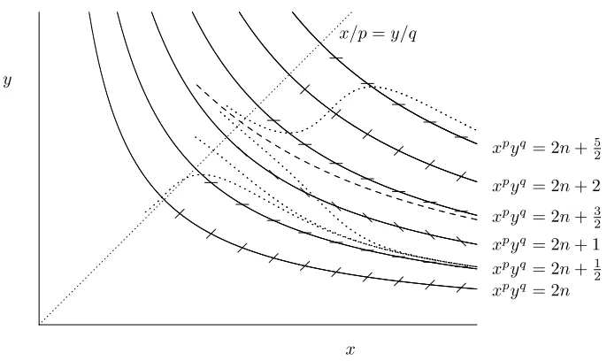
Some of the basic behaviour of the solutions of (2) can be understood by considering the lines in thex–yplane wherexp_yq_{is constant. The situation is shown schematically}

3 Solutions in the regionx/p > y/q 2

y

x

Fig. 1: Plots of solutions to (2) with y(0) = 2,4,6,8 and p = q = 1. The dotted lines in x/p > y/q show the curves xpyq = C to which these converge asymptotically asx→ ∞. The dashed lines inx/p < y/qgive the estimate of the mean path of the oscillatory part of these curves.

in figure 2. The arguments here are essentially the same as those in section 3 of Kerr, except the region is now divided by the linex/p=y/qand the lines under consideration are lines of the formxp_yq_=c.

If we consider lines wherexpyq= 2nthen solutions will have gradient 1 where they intersect these lines, similarly whenxp_yq_{= 2n+ 1 they will intersect with gradient−1,}

and whenxpyq = 2n±1/2 they will intersect with gradient 0. The gradients of the solutions will have gradients with magnitude at most 1, while the linesxpyq =cfor constantschave gradients greater than 1 in magnitude forx/p < y/q, and less than 1 forx/p > y/q. In the regionx/p < y/qsolutions must cross the linesxpyq=cfrom left to right, with a maximum each time it crosses a linexp_yq_{= 2n+}1

2,n= 1,2,3, . . ..

In the regionx/p > y/qthis restriction no longer holds. This results in the solutions having intrinsically different behaviour above and below the linex/p=y/q.

3

Solutions in the region

x/p > y/q

This is essentially the same argunment as previously in Kerr [2].

Any solution that enters a region 2n+1₂ ≤xpyq≤2n+ 1 is trapped in this region as xincreases as the gradient of a solution on the lower boundary is 0, and on the upper boundary is−1. Indeed, in such a region any solution that is initially above a

3 Solutions in the regionx/p > y/q 3

y

x

x/p=y/q

xp_yq _{= 2n}

xp_yq _{= 2n+}1

2

xp_yq _{= 2n+ 1}

xpyq = 2n+3₂

xpyq = 2n+ 2

xp_yq _{= 2n+}5

2

Fig. 2: Schematic plot for solutions in the regionx/p > y/q and the influences of the lines of formxpyq =c. The dotted lines show the trajectories of various solutions, while the dashed line shows the path of the separatrix dividing solutions that converge to xpyq = 2n+ 1/2 from those that converge toxpyq = 2n+ 5/2.

linexp_yp_{= 2n+}1

2 +will have a negative gradient of magnitude greater than sinπ

and so must eventually pass belowxpyq= 2n+1₂+, whose gradient tends to zero as

x→ ∞. Thus all solutions in this region asymptote to the linexpyq= 2n+1 2.

All solutions in the region 2n−1 2 < x

p_yq _<2n+1

2 will have positive gradients

and so will pass into the region 2n+1₂ ≤xpyq≤2n+ 1 from below, and will have one maximum in the regionx/p > y/q.

There is one solution in the region 2n+ 1< xpyq<2n+3₂ that stays in this region. Solutions initially below this curve will pass into the region 2n+1

2 ≤x

p_yq_{≤2n+1 and}

remain there, while those above it will end up in the region 2n+5₂ ≤xpyq≤2n+ 3. This curve is indicated by the dashed line in figure 2. By a similar argument to that given previously it can be shown that these seperatrices tend towards their asymptotes

xpyq = 2n+ 3/2 from below. We will denote the point where the separatrix crosses the linex/p=y/q as x/p=y/q=bn, and hence 2n+ 1< ppqqbpn+q <2n+ 3/2, or

(2n+ 1)1/(p+q)/(ppqq)1/(p+q)< bn<(2n+ 3/2)1/(p+q)/(ppqq)1/(p+q).

Clearly, any solution that ends up just above the curvexp_yq _{= 2n+}1

2 will have

crossedn lines given byxpyq = 1₂, 5₂, 9₂, . . .and so will have n maxima. Hence any solution that crosses the line x/p =y/q with bn−1 < x/p = y/q < bn will have n

4 Solutions in the regionx/p < y/q 4

4

Solutions in the region

x/p < y/q

As before, for large values ofy(0) the solutiony(x) will tend to oscillate quickly with small amplitude. The previous arguments hold here.

If lines of constantxp_yq _{=care given locally by the lines x+αy =C then the}

mean path of the oscillatory solution is given by dy

dx =

√

1−α2₋₁

α . (3)

The value ofαis determined by the curvesxp_yq_{=c. On such curves}

dy

dx =− pc1/q qx(p+q)/q =−

py

qx. (4)

Since the gradient of the lines x+αy=C is −1/α, we find α=qx/py and so the equation for the slope of the average curve is given by

dy

dx =

s

py qx

2

−1−py

qx. (5)

This has solutions

p

p2_y2_−q2_x2_+py

p

(p+q)y−pp2_y2_−q2_x2

p+q

= 2pppqp+qy(0)2p+q. (6) The solution curves meet the linex/p=y/qat the pointx/p=y/q=βwhen

y(0) = (p+q)

p+q 2p+q

22p+qp

β (7)

If thean are the values ofy(0) which correspond to thebn, and so are solutions

withnmaxima then we would have here

an≈

(p+q)2p+qp+q

2

p 2p+q

bn≈

2p+q1 _(p+q) p+q 2p+q_n 1 p+q 2 p 2p+q_p p p+q_q q p+q . (8)

5

Conclusions

We have used alternative derivation of Kerr [2] to analyse the generalisation the proiblem considered by Bender, Fring and Komijani [1]. With luk I’ve got the co-efficients right.

References

[1] Carl M. Bender, Andreas Fring, and Javad Komijani. Nonlinear eigenvalue prob-lems. Accepted for publication inJ. Phys. A, 2014.

[2] Oliver S. Kerr. On “nonlinear eigenvalue problem”. Submitted for publication in