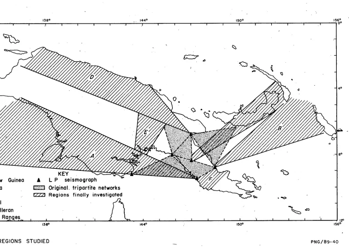
Rayleigh wave dispersion studies of crustal and upper mantle structure in New Guinea

(1)

RAYLEIGH WAVE. DISPERSION STUDIES • OF

CRUSTAL AND UPPER MANTLE STRUCTURE IN

Nbi GUINEA

by

J.A. Brooks, B.Sc.

Submitted in partial fulfilment of the requirements for the degree of

Doctor of Philosophy

UNIVERSITY OF TAMANIA

HOBA.RT

(2)

Except as stated herein, this thesis contains no material which has been accepted for the award of any other degree or diploma in any universitY, and to the best of my belief, the thesis contains no copy or paraphrase of material previously published or written by another person, except where due reference is made in the text herein.

(3)

CONTENTS

ABSTRACT

1. INTRODUCTION

1.1 SCOPE OF THE STUDY

1.2 CONTRIBUTIONS OF THE THESIS 1.3 TERMINOLOGY

1.4 BACKGROUND TO THE STUDY 1.5 THE PROJECT

Page viii 1 1 . 2 3 5

1.5.1 Conception 5

1.5.2 Eouipment 8

1.5.3 Seismometer housing 8

1.5.4 Field operations 9

1.5.5 Analytical Approach

1.6 DATA. 11

1.7 OTHER INVESTIGATIONS 11

2. SURFACE WAVE ANALYSIS • 15

2.1 GENERAL REMARKS 15

2.2 ANALYSIS

2.2.1 Data Processing Scheme 17 2.2.2 Phase Velocity Calculations 17

2.2.3 Profile Selection 18

2.2.4 Group Velocity 22

2.2.5 Inversion 23

2.2.6 The Inversion Programme 28 2.2.7 Interpolation of Model Solutions 30

2.2.8 Mantle Densities 31

2.2.9 Poissonls Ratio 33

2.3. ERRORS

2.3.1 Path Length and Origin Time 34 2.3.2 Variation of Initial Phase with Period 37 2.3.3 Variation of Initial Phase with Mode Number 38

2.3.4 The Time Window 39

2.3.5 Lateral Heterogeneity 40

2.3.6 Anisotropy 44

3. SOUTHERN NEW GUINEA 45

3.1 GEOLOGIC AND TECTONIC SETTING 45

3.2 OBSERVED DATA 50

3.2.1 Identification of Modes 50

3.3 RESULTS 54

3.3.1 Fundamental Mode 54

3.3.2 First Higher Mode 65

3.4 INTERPRETATION 72

3.4.1 Choice of Parameters 72

3.4.2 Inversion of Shear Velocities 75

(4)

ii

Page

4. THE SOLOMON SEA 84

4.1 GEOLOGY AND TECTONICS 84

4.1.1 Geophysical Data 86

4.2 OBSERVED DATA - 87

4.3 PHASE VELOCITIES 91

4.3.1 Paths to Popondetta 91

4.3.2 Paths to Tapini 96

4.4 GROUP VELOCITIES 101

4.5 DISCUSSION 104

5. NEW BRITAIN 105

6. NORTHERN REGION 113

6.5 CONCLUSIONS 122

7. THE CENTRAL CORDILLERA 125

7.3.1 . Event 11 128

7.3.2 Events 21, 46, 47, 59 131

7.4 CONCLUSION 135

B. OWEN STANLEY RANGE 136

9. REVIEW 141

9.1 METHOD AND TECHNIQUE ₁₄₁

9.2 RESULTS ₁₄₄

9.3 _{INTERPRETATION} ₁₄₅

9.3.1 The Upper Mantle ₁₄₆

9.3.2 Tectonic Hypotheses ₁₄₇

9.3.3 Regional Implications ₁₅₀

9.4 CONCLUSIONS ₁₅₃

(5)

Page

REFERENCES 157

APPENDIX I - SURFACE WAVE ANALYSIS 165 II - TRUNCATION OF A RAYLEIGH WAVE TRAIN 173

III - GROUP VELOCITY 188

IV - CONVERGENCE OF THE PHASE VELOCITY INVERSION

METHOD 196

V - SEISMIC WAVE VELOCITIES IN THE NEW GUINEA -

SOLOMON ISLANDS REGION (Reprint) 204

VI - INSTRUMENTAL RESPONSE 214

VII - SEISMOGRAM SPECTRAL ANALYSIS - SAMPLE OUTPUT

LISTING 229

(6)

_

iv

TABLES

1

2

Operational Periods of Field Stations

Percentage error estimates in phase velocity due to various errors in epicentral parameters for

Page

10

C = 4 km/sec. 35

3 Earthquake Source Data 51

4 Least Square Polynomials, Fundamental Mode 58 5 Fundamental Mode Velocity Studies 60 /

/6 Alternative Two Layer Models 62

7 Observed Velocities and Initial Phase Fundamental

Mode 63

8 Inversion of long period segments of Mphase

21

velocities 71

9 Observed Velocities and Initial Phase Mode M

21 73

10 Models SNG3 and SNG4 79

11 Earthquake Source Parameters, Solomon Sea • 89 12 Phase velocities for Profiles in Fig. 29 93 13 Model Parameters for Profiles in Fig. 29 98

14 Earthquake Source Parameters 119

15 Phase velocity data corresponding to profile lAt 119

16 Model parameters 120

17 Earthquake Source Parameters 130

18 Preferred solutions for event 11 131 19 Preferred solution for events 21, 46, 47, 59 133

• 20 Earthquake Source Parameters 136

21 Phase Velocities POP—PMG for event 7 140

(7)

ILLUSTRATIONS

FIGURE Page

1 MAP OF REGIONS STUDIED 4

2 TAPINI 6

3 SEISMOMETER INSULATION 6

4 GRASS THATCHED SEISMOMETER 'VAULT' POPONDETTA 7 5 CONCRETE BRICK, GRASS ROOFED•SEISMOMETER 'VAULT'

TAPINI 7

6 ANALYSIS FLOW CHART 16

-/ a. PARTIAL DERIVATIVES - Model Th 1. 25

b. INVERSIONS OF PERTURBED Th 1. 26

FOURIER SPECTRA OF UNPERTURBED AND PERTURBED

WAVETRAINS 41

9 RELATIVE PHASE VELOCITY DISPERSION PATHS 6, 13

TO TPN AND PMG ₄₃

10 SOUTHERN NEW GUINEA' EPICENTRES, PATHS AND CORE LOCATIONS

• 46

11 SHALLOW FOCUS EARTHQUAKES SHOWING WELL DISPERSED

HIGHER MODES 4$

12 DEEPER FOCUS EARTHQUAKES SHOWING STATIONARY GROUPS 49 13 TWO STATION FUNDAMENTAL MODE DISPERSION 55

14 EVENT 41. PHASE VELOCITIES 56

15 FUNDAMENTAL MODE PHASE VELOCITIES FOR ALL EVENTS 57

16 TWO LAYER MODEL INVERSIONS 59

17 GROUP VELOCITY DISPERSION, EVENTS 1, 41 61 18 COMPARISON OF OBSERVED AND MODEL M

21 GROUP VELOCITIES 64 19 SPAN OF PRINCIPAL LOBE OF VERTICAL DISPLACEMENT

PROFILE 66

20 OBSERVED AND G-B MODEL M VELOCITIES 68

21 OBSERVED AND MODEL PHASE VELOCITIES 70

22 SNG3 AND SNG4 SHEAR VELOCITY PROFILES ₇₄

(8)

vi

FIGURE 24A

24B

PHASE VELOCITY SENSITIVITY TO SHEAR VELOCITY, FUNDAMENTAL MODE

PHASE VELOCITY SENSITIVITY TO SHEAR VELOCITY, MODE 21

Page

""

78 25 DISPLACEMENT PROFILES FOR MODEL SNG4 80 26 SOLOMON SEA PATHS TO P OP ONDETTA , LAE 85

27 PATHS TO TAPINI 88

28 TYPICAL SEISMOGRAMS 90

29 DISPERSION PROFILES -FOR PATHS SHOWN IN FIG. 26 92

- 30 INVERSION SOLUTIONS FOR PROFILE II 94

31 INVERSION SOLUTIONS FOR PROFILE III 95

32 DISPERSION FOR PATHS TO TAPINI 97

33 DERIVED AND MODEL GROUP VELOCITIES 99

34 HAND ANALYSED AND MODEL GROUP VELOCITIES 100 35 GROUP VELOCITIES FOR PATHS TO POPONDETTA AND TAPINI 102 36 SENSITIVITY OF PHASE VELOCITY TO MODEL WAVEGU IDE

PARAMETERS 103

37 PATHS TRAVERSING NEW BRITAIN 1 106

38 FOUR GROUPS OF DISPERSION PROFILES 107

39 RELATIVE SEPARATION OF ALTERNATIVE PROFILES 109 40 RELATIVE SEPARATION OF ALTERNATIVE PROFILES 110

41 GROUP VELOCITY COITARISON 111

42 PATHS FOR NORTH COAST ANALYSIS 114

43 SPECTRUM OF EVENT 61 - LAB 115

44 SPECTRUM OF EVENT 74 - LAE 116

45 PHASE VELOCITY DISPERSION PROFILES, NORTH COASTAL

REGION 118

46 INVERSION SOLUTIONS FOR PROFILE 'A' 121

47 DERIVED GROUP VELOCITY DISPERSION 123

48 EPICENTRES AND PATHS FOR CORD I LLE RA N STUDY 126

(9)

vii

FIGURE Page

50 DISPERSION FOR EVENTS 21 ) 46, 47, 59 132

51 DISPERSION REGION COMMON TO PREFERRED PROFILES OF

FIGS. 49, 50 134

52 SOURCES AND PATHS - OWEN STANLEY RANGES 137

53 TWO STATION DATA, EVENTS 7, 14 139

54 VARIATION OF SHEAR VELOCITY IN THE UPPERMOST 50 Mq

143

(10)

viii

RAYLEIGH WAVE DISPERSION STUDIES OF CRUSTAL AND

UPPER MANTLE STRUCTURE IN NEW GUINEA

ABSTRACT

A study of Rayleigh wave dispersion from earthquakes within the New Guinea area has revealed two features of shear velocity distribution

not examined previously.

Variations in depth,to 300 km below the tectonically stable

-platform of southern New Guinea were determined from recordings of

funda-mental and higher mode Rayleigh waves. This average profile for paths

shorter than 2000 km, contains a low velocity zone reaching 4.2 km/sec. at

depths of 120 to 160 km, which is overlain by a relatively thick cap of

material with a velocity of 4.4 km/sec.

The lateral gross distribution of shear velocities beneath the

crust, emerged from examination of fundamental mode dispersion profiles.

Many of the phase velocity profiles were resolved from single station data

and techniques used to define the correct dispersion in such cases are

discussed. Although interpretations of these are strictly limited in

structurally heterogeneous regions such as New Guinea, phase velocities at

periods near 40 seconds are controlled mainly by shear velocities in the

uppermost 50 km of the mantle, in zones of greater homogeneity than the

crust.

Known geophysical data, existing hypotheses of geotectonic

development of the New Guinea region, the concept of sea floor spreading,

and observed characteristics of mineral assemblages under high temperatures

and pressures, provide a framework within which these data are examined.

Upper mantle Velocities are highest, about 4 ..7 km/sec., beneath

(11)

ix

southern New Guinea and appear to have intermediate values beneath the

cordilleran region. These differences are large enough to indicate that

regional variations exist in the mineralogy of the upper mantle.

The relatively low velocities underlying the southern New Guinea

crust may also imply a higher heat flow than normally expected in the most

ancient pre Cambrian shield regions of the world. -

In general the results are not sufficiently detailed or

compre-hensive to test existing hypotheses of geotectonic development of this

complex region and the study should rather be treated as a basic

contribu-tion to knowledge of the New Guinea area.

(12)

viii

RAYLEIGH WAVE DISPERSION STUDIES OF CRUSTAL AND

UPPER MANTLE STRUCTURE IN NEW GUINEA

ABSTRACT

A study of Rayleigh wave dispersion from earthquakes within the

New Guinea area has revealed two features of shear velocity distribution

not examined previously.

Variations in depth_to 300 km below the tectonically stable

platform of southern New Guinea were determined from recordings of

funda-mental and higher mode Rayleigh waves. This average profile for paths

shorter than 2000 km, contains a low velocity zone reaching 4.2 km/sec. at

depths of 120 to 160 km, which is overlain by a relatively thick cap of

material with a velocity of 4.4 km/sec.

The lateral gross distribution of shear velocities beneath the

crust, emerged from examination of fundamental mode dispersion profiles.

Many of the phase velocity profiles were resolved from single station data /

and techniques used to define the correct dispersion in such cases are

discussed. Although interpretations of these are strictly limited in

structurally heterogeneous regions such as New Guinea, phase velocities at

periods near 40 seconds are controlled mainly by shear velocities in the

uppermost 50 km of the mantle, in zones of greater homogeneity than the

crust.

Known geophysical data, existing hypotheses of geotectonic

development of the New Guinea region, the concept of sea floor spreading,

and observed characteristics of mineral assemblages under high temperatures

and pressures, provide a framework within which these data are examined.

Upper mantle Velocities are highest, about 4 . .7 km/sec., beneath

(13)

1. IIIIRODUCTION

1.1 SCOPE OF THE STUDY

This thesis presents interpretations of recordings of dispersed

Rayleigh wave trains for several paths in the New Guinea area. Results

. include "crustal" thicknesses and upper mantle shear velocities found by

numerical inversion of phase velocities relating to the six regions marked

in Fig. 1, and are presented against the background of previous geological

and geophysical studies of the region.

3

1.2 CONTRIBUTIONS OF THE THESIS

I believe the work offers contributions in two respects. Firstly,

it provides new data for a part of the south west Pacific area not specifically

examined geophysically, in a regional sense, until the present decade. Secondly,

and from a seismological point of view, four aspects can be mentioned:

(i) It is useful to be able to describe the earth in terms of

regional transfer functions for various kinds of

transmiss-ion, irrespective of the interpretations made in terms of

physical models. In this study, phase velocity dispersion

profiles are derived for several small regions, some of

them structurally heterogeneous on a pronounced scale.

While velocities remain the most widely studied parameter

of travelling surface waves, dispersion profiles comprise

the most useful part of the transfer function. No

informa-tion about path attenuainforma-tion is deduced here.

(ii) Usually, the depth to which structural information is

(14)

decreases. Therefore, data which provide good penetration

over short paths are extremely useful. The higher modes

of surface wave transmission offer such a facility (Kovach

and Anderson, 1964), and this study presents a shear

velocity profile to a depth of 300 km for path lengths of

between 1000 and 2000 km. Similar profiles for regions

elsewhere e.g. Brune & Dorman (1963) involved much longer

paths. The profile for southern New Guinea discussed here,

depended on the analysis of higher mode Rayleigh waves

. which, simultaneously with the fundamental mode, controlled

the numerical interpretation.

(iii) A feature of the analysis is the reliance placed on "single

station" phase velocities, requiring an examination of the

source phase term and its frequency dependence. The

approach adopted was strictly empirical. Group velocities

were used to determine the magnitude of the source phase

• term, and the small degree of its variation with frequency

was demonstrated by close agreement of several events.

The evaluation of crustal thickness employed a variation

of the numerical inversion technique by using Poisson's

Ratio as a criterion to establish a preferred solution.

1 .3 TERLIPTOLOGY

Definitions given by the American Geological Institute (1962) have

(15)

1.4 BACKGROUND TO THE STUDY

In 1958 I was appointed to direct the Port Moresby Geophysical

Observatory during its establishment and early years of operation. One of

the main tasks of the Observatory involved routine seismological recording,

and it soon became obvious that the future activities of the establishment

would have a strong seismological bias because of the intense seismicity of

the New Guinea-Solomon Islands region.

At that time, no regional geophysical studies of this tectonically

complex region were known to me ., and facilities were inadequate to provide

nx.

a-basis on which regional structure could be examined-seismologically. An

early attempt is represented by Appendix V of this thesis (Brooks, 1962).

I presented these findings to the Tenth Pacific Science ,congress, Honolulu,

preceding a brief visit to California in 1961. During my visit to the

Seismological Observatory at Pasadena, my interest was aroused by Professor

Frank Press in the possible use of surface waves as an economic, effective

tool for studying gross crustal and upper mantle structural variations, in

circumstances such as than existed in New Guinea. Such a program for the

European Alpine region (Knopoff & Press, 1961) had recently commenced. On

my return to Port Moresby a similar proposal was devised and its aims

outlined by Brooks and Ripper (1966).

The equipment was delivered in 1964, field recording began in 1965,

and culminated in the preparation of this thesis.

It was apparent, quite soon after the first.records were made, that

hand methods of analysis would not suffice, although no computing facilities

were then available in New Guinea.

However, in 1965 I was granted a two year post-graduate Scholarship

to the University of Tasmania, Department of Geology, by the Commonwealth

Public Service Board with the support of the Director, Bureau of Mineral

(16)

132° 138°

0° _{:r 1} 144° 150° 156° 0°

4° ₀ 4°

KEY

Guinea A L P seismograph

=3 Original, tripartite networks

=23 Regions finally investigated

REGIONS

A. Southern New

-8 Solomon Sea

C New Britain

_D North Coastal

\,.E Central Cordilleran

F. Owen Stanley Ranges

• •Gs

120 12°

138° 144° 1500 156°

132°

[image:16.832.137.820.45.533.2]

( Based on A/BO-22) (F140/130-25)

(17)

becoming available. The venue was chosen at the invitation of Professor

S. Warren Carey because the proposal combined well with his stimulating

Papua-New Guinea Tectonic Project. This comprehensive multiple

investiga-tion was designed by Professor Carey to collate, supplement and interpret

existing unpublished geological and geophysical data held on exploration

company and government files, especially the Bureau of Idineral Resources.

The geological phase of the project is represented by the unpublished

theses of Smith (1964) , (1966) and Kugler (1968).

The surface wave project was incorporated in the geophysical

has of the study represented in addition, by gravity studies of Shirley

(1964) and St. John (1967).

1.5 THE PROJECT .

1.5.1 Conception

The original field program was designed to measure phase

veloc-ities across triangular networks of single component long period vertical

seismometers, after the manner of Press (1956) and Knopoff & Press (1961).

A schedule was devised to allow four to six months occupation of

each network, followed by relocation of one or more seismometers to cover

a new area. Station locations were chosen so that, as far as possible, the

regions covered by each network did not include parts of two radically

different topographic, and hence structural, units, e.g. shield, cordilleran,

oceanic. Communication and especially transport difficulties in the

Territory also .constrained the choice of station locations, shown in Fig. 1.

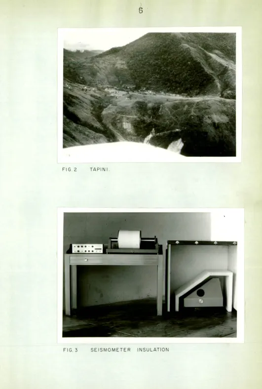
Fig. 2, of the Tapini outpost illustrates the difficult topography of some

(18)

[image:18.558.13.544.12.800.2]

FIG 2 TAPINI

FIG 3 SEISMOMETER INSULATION

(19)

S

EISM

O

M

E

TE

R

POPO

NDET

TA

G

RASS

TH

ATCH

ED

SEISMO

ME

TE

(20)

1.5.2 Equipment

The problems of operating, remotely and indirectly, long period

seismographs in tropical conditions, governed the choice of equipment and

outweighed the desirability of including three component instruments. The

equipment chosen was:

Seismometer: SV-282 Press-Ewing type (UED) T o = 15 sec.

Critical damping was employed.

Recorder : ER-230 Pen recorder (UED) employing a passive filter. System

response is discussed in Appendix VIbut is similar to that of --

the World Wide Standard equipment. A recorder drum speed of

60 mm per minute was chosen for good time resolution.

Timing : Crystal oscillator controlled timing and power units, model

NCD2 were especially designed and built in the B.M.R.

labora-tories for the project (Jones, 1968). They provided 40 w. of

regulated power to drive the recorder.

This unit employed a pulse count comparator and display

unit, calibrated in milliseconds to facilitate measurement of

time errors by non-technical operators, and maintained

chronometer rates of a few tens of milliseconds per day.

1.5.3

Seismometer housing

Considerable thought was given to this because of the extreme

temperature sensitivity of long period seismometers employing the

"zero-length" spring. Planned technical inspections of ecuipment at

3

week

intervals required the seismometer to operate without the need to readjust

the pendulum during this interval. Fig.

3

shows the double unit insulation

system which in turn was housed in temporary structures of the type shown

in Figs.

4

and

5.

These structures employed local building materials, were

(21)

1.5.4 Field Operations

Daily routine duties were undertaken by Papuan orNew Guinean

attendants employed locally. Special consideration was given to the design

of a log sheet to show details of the record change, time comparison and

step function calibration, in the most direct manner, with •a minimum

possibility of errors.

Technical servicing of field stations was carried out by personnel

from the Port Moresby Observatory. /-

/

1.5.5 Analytical Approach

The planned interpretation of tripartite recordings failed for two

main reasons:

(i) Wavetrains from sources outside the New Guinea region were

disturbed before reaching the recording area, by interference

from laterally reflected and refracted wavetrains with the

parent wavetrain. Pilant and Knopoff (1964) and Knopoff et

al, (1967), discussed some aspects of this problem. The

phase errors were large enough to dominate the phase shift

over such a small network as Port Moresby-Tapini-Popondetta.

Extreme selectivity of seismograms was needed to obtain data

of even moderate quality. Apart from the structural

varia-tions of tectonic units surrounding the region, in all

azimuths, the irregularly shaped coastline of the island of

New Guinea itself introduced added complexity to the problem.

(ii) Logistic problems encountered in the maintenance of field

stations prevented the required continuity of recording by

three stations simultaneously, and the large quantity of

(22)

1

0 •

These difficulties were being recognised when it became clear that

.similar problems had arisen with a similar type of structural analysis of

the European Alpine region (Pilant, Mueller & Knopoff, 1966) which had

commenced in 1960 (Knopoff & Press 1961).

Late in 1966 I decided, because suitable data was lacking, to

change the emphasis of the project to an analysis of records of earthquakes

occurring within rather than outside the New Guinea region.

The disadvantage of this approach was that single station records

were employed, requiring investigation of the source phase term, and

consid-eration of travel time errors due to limited accuracy of path lengths.

Furthermore, structural information was averaged over regions much larger

than covered by each original tripartite array.

TABLE 1

Operational Periods of Field Stations

STATION ABBREVIATION PERIOD OF OPERATION-

Port Moresby PMG May 1965 - May 1967 )

Popondetta POP May 1965 - November 1965

Tapini TPN May 1965 - February 1967

Kerema KER February 1966 - March 1967

Daru DRU • February 1966 - October 1966

Lae LAB December 1966 - May 1967

By contrast however, a much wider range of structures could be

examined and the new technicue also offered more originality

(i) in employing near earthquakes, i.e.A4:1 1000 km, for the

first time.

(ii) in the method used to estimate the source phase.

(23)

1

Fig. 1 compares the regions finally investigated with the original

proposals.

The periods for which various stations were occupied are disclosed

in Table 1 without detail ihdicating periods of satisfactory or unservice-.

able operation.

1.6 DATA

A total number of 127 seismograms involving 80 sources was digit-

- ised at intervals of 1 or 2 . seconds, depending on the record character.

53

of these source - station paths were used in some way during

interpretation of structure beneath the regions shown in Fig. 1.

A catalogue of source, mode and path information for these data

is given in subsequent chapters where each region is discussed.

1.7 OTHER INVESTIGATIONS

Before 1960, information about the tectonics of the New Guinea

region was represented, almost solely by the work of Stanley (1923), Carey

(1938 a l b), van Bemmelen (1939), David (1950) and Glaessner (1950).

- Even now, few publications have dealt quantitatively with the

gross crustal structure of New Guinea. Most of what, is known, or currently

accepted, has emerged as a by product of extensive geological and geophysical

oil search activities undertaken both in the western and eastern sections of

the island, and is mainly confined to the upper five kilometres or so of the

Thrust, e.g. Vi,ser and Hermes (1962), APC (1961).

Recent studies fall into three categories:

(a) Those comprising the Papua-New Guinea Tectonic Project,

(24)

12

tectonic analyses by Smith (1964), Pitt (1966), Kugler (1968), .

the gravity study of Shirley (1964) and the comprehensive

analysis of the regional gravity field and tectonic synthesis

by St. John (1967).

(b) A series of geological reports by the Bureau of Mineral.

Resources covering several regions within eastern New Guinea,

and summarised by Thompson and Fisher (1965).

(c) Isolated seismological studies e.g. Brooks (1962) - P & S

velocities; 'Doyle & Webb (1963) - Pn residuals; Brooks (1965,

a,b) - seismicity; Brooks & Ripper (1960 - group velocities;

Denham (1968) - crustal thicknesses.

An early analysis of special interest by Visser & Hermes (1962)

included a hypothetical profile of the lower crustal boundary from the

southern to the northern coast of West Irian. Crustal thicknesses ranging

from 10 to 20 km off the north coast to about 40 km under the Van Rees

Mountains and central range areas, thinning to 30 km or more under the plains

of southern New Guinea were associated with a Bouger anomaly profile ranging

between +100 mg. Visser & Hermes disclosed extensive thicknesses of

sedi-ments extending to the top of crystalline basement at depths of five or more

km.

The gravity implications of similar basins in eastern New Guinea

comprising the southern marginal elements of the Papuan Geosynclinal System

(Smith, 1964) is discussed by St. John (1967) whose analysis was based on a

standard crust of 35 km beneath the zero Bouger anomaly contour in southern

Papua, and a crust-mantle density contract of 0.5 gm/cc. These basins are

sufficiently extensive to affect Rayleigh wave dispersion (Brooks & Ripper

1966). According to St. John, crustal thickness variations exceeding 25 km

occur between the central cordillera and the Solomon Sea.

Rose, Woollard and Malahoff (1968) have made a preliminary

(25)

13

employing a crust-mantle density contrast of 0.46 gr/cc and a standard

32 km crustal section. Departures from zero Bouger anomalies were then

interpreted as a function of water depth free air anomaly and Crustal

thickness. Estimates of thickness ranged from 5 km under the trench west of Bougainville, to 10 km under the central Solomon Sea basin and 20 km

under Bougainville Island.

Reinforcing the overall picture of regional instability apparent

from the high seismicity, these studies of the gravity field provided strong

evidence of variations in gros crustal structure within New Guinea.

Seismology has contributed little to an understanding of this

structural problem. Some inferences as to the probable broad characteristics

of the crust both north and south of New Guinea have been drawn. Kuo et al

(1962), in discussing broad categories of crustal structure in the Pacific

Basin,. inferred from Rayleigh wave group velocities, commented that the

Melanesian-New Zealand area west of the Andesite line showed distinctively

different characteristics from the Pacific Basin proper. Specifically they

noted that the path between the Banda Sea and Fiji represented neither a

typically oceanic nor continental structure.

A comprehensive study of group velocity dispersion observed over

a number of intersecting paths in and around the Pacific led Santo (1963)

to infer that the crust immediately to the north and south of New Guinea was

chiefly continental in broad characteristics. Brooks & Ripper (1966) noted

an apparent progressive thickening of the crust for a sequence of paths

radiating from Port Moresby, southwest to the West Australian coast, west

to Timor and finally northwest across the New Guinea Cordillera. This

conclusion was subsequently supported by the gravity data (St. John, 1967). Earlier, Doyle & Webb (1963) had studied Pn residuals at Rabaul

and Port Moresby from Pacific nuclear explosions, and concluded that a

'continehtal type' crust underlay Port Moresby and an 'island type' crust

(26)

14

(27)

1_5

2. SURFACE WAVE ANALYSIS

2.1 GENERAL REMARKS

The purpose of this chapter is to examine the analytical approach

employed in this investigation and review the important sources of error or

misinterpretation associated with dispersion studies, particularly those

relying on the "single station" technique.

The theoretical and observational basis for the extensive surface

wave-investigations of the last decade is well established in the literature.

A decade ago, analytical reductions were still largely dependent on hand

analysis methods to measure dispersion and were confined to well dispersed

wavetrains. Interpretations were comparatively crude and confined to simply

structured waveguides with one variable parameter (usually thickness). The

effects of lateral heterogeneity, anisotropy and source characteristics have

only recently received attention. -

Phase velocity measurements have supplanted the earlier reliance

on group velocity, and may be determined in several way 4 employing one or

more stations. Investigations of structures beneath the Canadian Shield by

Brune and Dorman (1963) and the European Alps by Knopoff et al (1966), provide

good illustration of the use of two and three stations respectively. Networks

with more stations have been used by Aki (1961) and Alexander (1963). The use

of multiple stations allows measurements over small areas, with dimensions of

the order of a wavelength, provided the waveguide is sufficiently homogeneous

that phase errors, of the kind disclosed by Knopoff, Berry and Schwab, (1967) ₎

are avoided.

Apart from the work by Brune et al (1960) and Dab et al (1962) _/

single station methods have not really been trusted because of source

(28)

16

SEISMOGRAM STEP RESPONSE

DIGITISE

V

NUMERICAL FOURIER TRANSFORM LAGUERRE

FUNCTION EXPANSION

FOURIER TRANSFORM

'SOURCE AND PATH DATA

ALTERNATIVE C:T CURVES

00= = ncr

2—LAYER - MODEL INVERSIONS

GROUP VELOCITY

a = Hand analysis b Bandpass filter c = Polynomial

differentiation

MODEL GROUP VELOCITIES

IDENTIFY CORRECT 00

COMPOSITE INVERSION OF M11, M21

[image:28.556.61.525.29.810.2]

DATA

FIG. 6. ANALYSIS FLOW CHART

(29)

17

2.2 ANAIYSIS

2.2.1 Data Processing Scheme

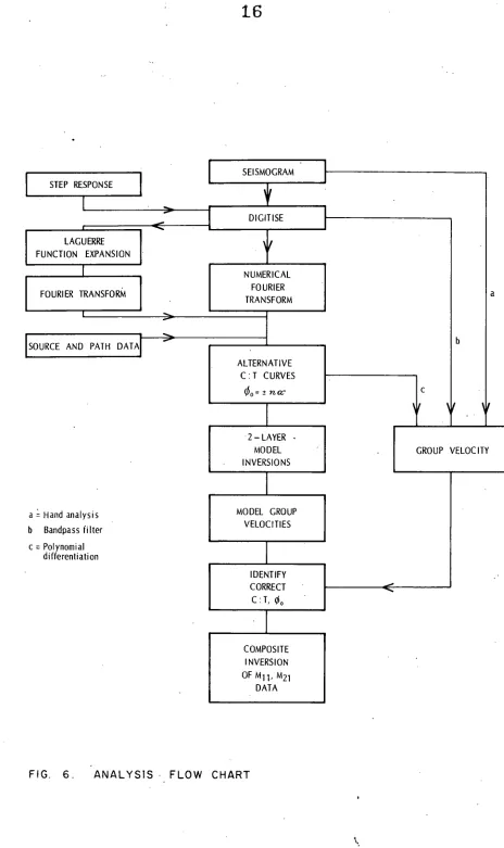
A diagrammatic illustration of the analytical approach is shown

in Fig. 6. This was not wholly automatic, as results required subjective

assessment at intermediate stages.

2.2.2 Phase Velocity Calculations

Phase velocities were computed from the Fourier spectrum, F(),

of each digitised Rayleigh wave train, f(t).

Thus, for a plane wave front, the phase angle, o(Lo) (relative to

- some defined origin) of a particular frequency,w(radians/seco) can be

shown to be (Appendix Ia),

op).

- kr + 0 (64 + 00(co)

where t = interval from origin time to beginning of wave train

k = wave number =w1C(40), C = phase velocity

95(w) = phase delay introduced by the seismograph system

.0

(,u) =

apparent initial phase at the source 0

r = epicentral distance (kms)

Solutions for the displacement potential of a disturbance originating from

a point or line source, i.e. spherical or cylindrical waveforms, require an

additional nett phase correction of 774 sometimes called the "spreading

correction" (see Appendix Ib). Thus from (1), the phase velocity is given

by

C(co)

= WrAtob - OH+ 0(4+0060 + T`74 1

(2)

0

(4)) was first determined by a Fourier-Laguerre transformation 0

(Dean, 1964) of the seismograph step function response which was recorded

daily. (Appendix VI).

(30)

numerical integration routine (Appendix ia), and listed out with the

trans-form. Usually

e

traversed several cycles for the period range 15 to 60

seconds.

• -0(4 was computed at standard frequency intervals of 0.002 cycles/

sec., sufficiently small so that the phase difference between adjacent points

was always less than a full circle.

Calculation of a family of phase velocity profiles commenced at the

• long period end of the spectrum at a frequency,, selected beforehand by

inspection of the record. In the case of the fundamental mode, L) usually

ranged between .014 and .03 cycles/sec. A trial CM was first computed from

0(c4.9. The angle was then varied by increments of ri until a value of C(40

between, or nearest, the interval 3.80 to 4.10 km/sec. was found. A. family

of dispersion curves was computed for each event by arbitrarily assigning to

0

0 , incremental values corresponding to -± nog n = 0 1, 2; do: =IT/a so that phase velocities remained within a physically plausible range e.g. 3.5 to 4.5 km/sec. for the fundamental mode in the pd'iod range 40 to 70 seconds. Brune et al (1960) shows several examples of such families of curves. The

choice of oc is discussed below.

Program output (Appendix VII)took the form of an optional listing

of the Laguerre coefficients and step function frequency transform followed

by the Rayleigh wave transform and the table of alternative phase velocity,

profiles together with initial phase. The frequency range covered by the

transform and the velocity profiles were controlled by variables set

follow-ing a visual examination of each record to estimate the part of the spectrum

containing useful amplitudes.

2.2.3 Profile Selection

(a) Choice of Initial Phase Increment (oc.)

(31)

1.

9

to compute dispersion curves, and corresponding models, bridging or closely

approximating, the correct carve. There have been. fe;y "single station"

analyses which have relied on postulated values of ₄ . One such example is

that of Kuo et al (1962) who considered values of ± n71/2 for Rayleigh waves

in the period range 20-140 sec. The paths used were several thousand km long

and consequently their . possible alternative dispersion curves were separated,

even at the long period end, by only very small velocityincrements making

a confident assignment of 00 a difficult exercise.

The source parameter-A2 has been examined both theoretically and

---empirically by several workers.

Brune et al (1960) established pLII:n/T (n=0, 1)2-) in model studies

in which a spark discharge provided the source, and applied this result to

study Rayleigh waves from nuclear explosions. Its application to earthquake

records would seem justified if the source were shown to be of basically

impolsive or explosive type, and there have been ''liggestions to this effect,

e.g. Evison (1967).

Others have tested the more widely held hypot,hesis of a fault

(shear failure) source having a basic single or double couple action.

Aki (1960) et seq, used cross correlation techniques to estimate

A

to within about 714. His definition of does not include the spreading

correction, thus 0.= A(ki)- 74. Aid (1962) summarised the derivation of

from Lamb's 1904 studies of horizontal and vertical displacements due to

impulsive sources, and extended the findings to the strike and dip slip cases

and found 00=0,ir (strike slip) and 44)0=± 71/ (dip slip).

Haskell (1963) theoretically derived the radiation patterns expected

from fault-type sources disposed in a variety of attitudes, adopting the

convention for

0

employed by Brune et al (1960). Apart from one example

(Haskell (1963, p.635)),00 appears very close to 2: nyafor the extensive range

of cases studied. Departures from this value are discussed in Appendix. I(b).

(32)

20

apparent azimuthal variation have involved only long period (T> 100 sec.)

fundamental mode waves. The work of Brune et al (1961), Brune (1962) and

Chander and Brune (1965) hOwed 0i) =:tn,72 for most azimuths, departures being

confined to °cross-over regions" bridging the azimuthal fields of constantA.

Thus almost all investigations have disclosed A to have values

which are integral multiples of %. for all azimuths except the

narrow,azi-muth ranges surrounding the "cross-over regions". Therefore c<=%._ has been

adopted, and found a satisfactory increment for A, in this study. For the

range of epicentral distances-.,Qmployed, adjacent dispersion curves are

,usUally sufficiently separated so that (a) corresponding models are distinct- ,

ive, and (b) an unambiguous indication of the correct

A

is given by

super-imposing sets of dispersion curves corresponding to different distances.

In this study the source - station paths are all similarly directed

and epicentres are not widely separated. If the earthquake mechanism is

tectonically controlled, one might expect similar values of A measured in -

the same quadrant.

(b) Identification of Dispersion Profile

The need arises now to identify the correct dispersion from the

several alternatives available.

This is achieved either by comparison with two-station data, as

in Chapter

3,

Fig. 13, or by the scatter of points in the superimposed plot

of sets of alternative profiles for several events.

Consider two events, and corresponding path lengths r

1 and r2'

beneath which the waveguide is identical. Initial phase angles at the source,

00

in section 2.2.3, are 0, 1 and 002. .

Let A I and 0, 2 :respectively be the values of initial phase,r07A ,

adopted in each case. For particular choices of n, different for each event,

and 012. can be so chosen that

k'f0, = 950,

(3)

(33)

21

define the true discrepancy in adopted source phase. Travel time errors

for waves of period T are

=

T ,A116,

and _2. T 6,0z

2.Tr 2,7

and resulting errors in phase velocity are

=

2 Tr t, a

and LA, Ca —T A , coz r-

2 -rr

Assuming that IL -- I , where t12.

AC—ACT₁₂

(rØ

-r)

212. 1 11

a71 (5

)

Alternative values of phase velocity are defined by incremental changes of

T1 and n2 . Thus from (3), (4)

A 0-(11

and

a a a

and, from (5)

Aa C i — Aa Ca

_=AC

,Ia

T (r-

2 ;(. ri)

Zut

z

a

Hence for each incremental change of A I , 91 2 , the corresponding members of

each set of profiles become further separated by incremental amounts

_I

h-n).

47rE.'

The standard deviation from a mean curve placed through each pair

of profiles correspondingly increases, and this applies also to sets of more

than two profiles.

Other errors considered below, (2.3.1), also exist, but are not

dependent on

06

and thus do not significantly influence changes in standard deviation resulting from changes in

Ø. Fig. 14, Chapter

3,

illustrates the changing separation in the case of 2 events and Table 4 and Fig. 15 the

increasing standard deviation within sets of profiles progressively removed

from the correct dispersion curve.

Hence, a set of profiles having a "mean" profile, closer to the

true average dispersion than any other set, will also show a smaller standard

deviation from its mean than any other set. Alternatively two sets may

(34)

22

"straddle" the true dispersion curve in which case, the standard deviations

will be nearly equal, and smaller than sets above and below them.

In practice, careful inspection is sometimes required to correctly

group members in corresponding sets. Most difficulty arises where the path

distance and origin time errors, section 2.3.1, are sufficiently large to

distort the relative separation between profiles for events having nearly

equal path lengths, for example, as in Chapter 4. To this extent, the

pro-file matching procedure is subjective. Provided these supplementary errors

vary in sign and magnitude for each earthquake, increased protection against

their distorting influence, is afforded as the set of.. events used increases

in size.

Correct matching is impossible if these supplementary path and

distance errors are so large that discrete groups of profiles become "smeared"

together. In practice this did not occur for any set of paths studied-,

2.2.4 Group Velocity

If

it= (.0:64

is the wave number, then group ,./elocity is given,

_from equation (1), section 2.2.2, by

(ca) rir

f t-

e

i

(

t,J)

+15 tw) + 00

i

(

w) (5) Thus b =

-

is defined as the group travel time.

Hence, whereas phase velocity depends on the source phase angle

group velocity depends only on variation of with frequency. This is

usually very small, and can safely be ignored.

The three methods used to calculate 1.)(60 are explained in Appendix

III. They are:

(1) The simple and conventional hand analysis method, which is

satisfactory provided the dispersion is not too rapid.

(2) The digital filter technique devised by Alexander (1963).

(35)

23

higher modes at periods less than 30 sec.

(3) Direct differentiation of a polynomial fitted to sets

in a Chebyschev sense. This proved useful provided the phase velocity profile was known over a large period range

includ-ing long periods.

Fig. 6 schematically illustrates how group velocities were used to select the correct phase velocity profile (and hence initial phase) from the families of such curves (section 2.1.2 above).

'Group velocity profiles were computed from models found by inverting _.-various phase velocity profiles, and then compared with group velocities

derived or measured directly.

2.2.5 Inversion

Methods of inverting phase velocity data to provide layer parameters of a hypothetical model having equivalent disperdion properties to those

observed was first demonstrated by Dorman and Ewing (1962), and has since been applied by others. Brune and Dorman (1963) inverted bOth Love and Rayleigh - fundamental modes to establish their CAN-SD model for the Canadian Shield.

McEvilly (1964) tried a similar approach for the central U.S.A. and could not find a model compatible with both modes. Berry and Knopoff (1967) using fundamental 'Rayleigh mode data of only limited precision, found a model for the western Mediterranean. -

Brune and Dorman (1963) list some important restrictions associated with the approach which, while not permitting a unique reduction does offer a less arbitrary interpretation of a phase velocity dispersion profile than previously available. These restrictions are to some extent a consequence of the part dependence of compressional and shear velocity and density on each other.

(36)

Dorman and Ewing (1962) and the other authors mentioned above.

The partial derivatives DCA9i , rt of the n active or 'floating' parameters in a particular model, comprise the matrix of coeffic-ients of the set of equations of condition for each of the m values of observed phase velocity. These are to be solved for corrections

DC

i.e.

.d

L.4-1=/ 5-A•

_ cU _{) J} _{where the dC•}

are the differences between observed and model phase velocity.

Freedom to adjust the.model is restricted in - the following ways: (i) Two or more parameters, p, should not be varied

simultane-ously if profiles of phase velocity sensitivity,

aqap

as a function of period have similar or reversed outlines. (ii) A parameter should not be allowed to vary in a particular

problem if the maximum sensitivity ()Op is much less than the known precision of the data,LIC. There is no point in adjusting

p

closer than AC/ (C/af)

(iii) Successive iterations of a particular problem must produce a convergent solution. If this requirement is not met; succ-essive iterations produce models which match the observed dispersion equally well while containing physically unre

a

l-istic layer velocities, densities or thicknesses.

Conditions (i), (ii), and (iii) express different aspects of a common problem of numerical instability associated with the use of the inversion technique.

Under conditions (i), above, the matrix of coefficients can approach singularity causing instability in the resulting solutions. For example the requirement prohibits the simultaneous adjustment of shear velocities and densities of the same model. If two such parameters are varied, especially where the sensitivity of phase velocity to one is much greater than the other,

(37)

0-2 -1.0

8c/8/6/

0. 04

8 c

/ er/

0.

( KM/S/KM/S )

8c/ 48/ KM/S/KM/S

-

8c

/8a,

—esc

4h, - 0-02

ac/sh

,

KM/KM/S

- 0-0/

0 —0

[image:37.830.42.760.65.534.2]

15 25 35 45

FIG. 7A PARTIAL DERIVATIVES OF PHASE VELOCITY WITH RESPECT TO

(38)

0-15 025 0.35

42

40

(KM)

1

38

36 WM.

a

1

A 0

34

/

3

3.0

[image:38.833.83.787.47.531.2]

5.0 a

FIG 7B INVERSIONS OF PERTURBED MODEL

4•0 5.0

6.0 70

VELOCITY (KM/S)

Th I FOR CRUSTAL THICKNESS 610 VALUES 36,38, 40 KM, \.

(39)

27

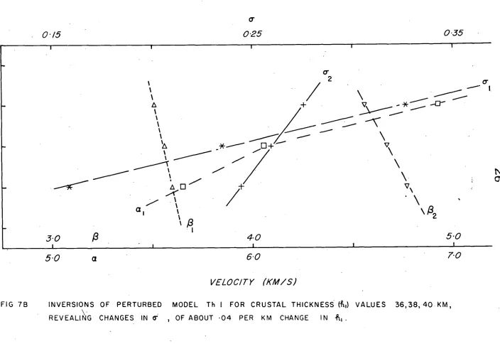
which does not stabilise after a few iterations and develops a tendency to Such "hunt" in response to small changes in the more sensitive parameter. ouch. a pair are thickness and compressional velocity of the upper layer for 2 layer crust-mantle model. This particillar model is widel y used in this study to establish average depths to the M-discontinuity and the problem of realising a stable inversion was overcome in the following way:

Moho depths were determined by repeated inversion of data covering a restricted period range, in terms of a 2 layer model i.e. crust over semi-infinite mantle. In each inversion a different fixed value of crustal

thick-/

ness (h

1) was used while crustal velocities c< 1 01, and mantle shear velocity, (42 , were allowed to vary.

The unknown error in h

1' is absorbed mostly by or, because the shapes of the respective sensitivity: period profiles are similar, and partly by 0 1 because oc, and ft, are not quite independent.

Using the relation

to find Poisson's Ratio 07, it is easy to verify the statement of Hanamori and Mizutani (1965) expressing sensitivity of

6-1 to small changes Zioc, and 4,

i.e. 4 crial 3 flApcpc,I + 14(31/(3,1}

i.e. an error, Ckk, , causes an apparent variation, 2kr; , thus

30c/0(1311,)/

0a + 100,

WOO

_{lj a}

_h,

The partial derivatives C.PhDCPcg, 30(3

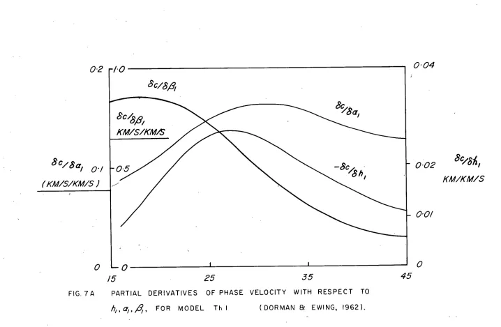
1 to use in this formula can be obtained from a "representative" model. Those for Dorman & Ewing's (1962) model Th1 are shown in Fig. 7a., Representative values of .03,

.15, .5, respectively indicate that a change of about .04 can be expected in

GI for each 1 km change in crustal thickness as shown in Fig. 7b. This

figure would vary slightly for different models, but provides a convenient crit-erion to establish la

(40)

28

•determination of optimum layer thicknesses is not easy but can be assisted partly by considering the shape of the displacement profile for a given mode and model as an adjunct to the sensitivity profiles. The amplitude profile

(either vertical or horizontal component of displacement) should change appreciably over the depth range of a particular layer whose parameters are

to be adjusted. Some protracted, but essentially simple tests were performed with synthetic data (Appendix IV). In these tests, phase velocities were computed for a 5 layer upper mantle model having layer thicknesses of 50 km or more. These velocities were then treated as observed data in four sets of inversions. The velocities were accepted at 5 place accuracy and also rounded

to 2 decimal. places. For each case, the model shear velocities were perturbed by setting them to a common value of 4.5 km/sec. Initial reductions were found for models in which layer thicknesses were unaltered. Additional tests, using models for which layer thicknesses were halved, were then made. Results

given in the appendix clearly illustrate an instability for models with the split layers which was very slowly overcome only when the "observational" data was given to 5 places of decimals. Instability did not appear in the initial set of reductions, even with "observational" data given to 2 places of decimals.

2.2.6 The Inversion Programme

The program employed was developed from the version called IW3 written for an IPM 7090 computer (Fortran IV) by Brune and Dorman for their •Canadian Shield investigation. This employed the Haskell matrix subroutine

for calculating dispersion used in Dorman's program PV7 referenced by McEvilly (1964) and Mooney & Bolt (1966).

INV3 was translated into ;lgol for running on the Elliot 503 com-puter

OK

random access store) available at the University of Tasmania. Several modifications were made.

(1) The earth flattening approximations of Alterman at al (1960) were added to allow inversions of the M Rayleigh mode phase

(41)

?9

velocities. This increases the shear and compressional

velocities of layers according to the following formula

k -u- +

Ir = modified compressional or shear velocity in layer

= assigned velocity in the flat layer model

= depth to mid point of the layer

R

= Earth radius

This increase in velocity compensates for the smaller travel

path for portions of deeply penetrating waves in the real

earth.

These adjustments were made before calculating the model

phase velocities and partial derivatives in each iteration.

Corrections from the solution of normal equations were applied

to the flat-layer model velocities and final solutions given

in terms of such a model.

(2) The matrix inversion sub-routine of INV3 was replaced by a

faster "forward and back substitution methcd" of solving

symmetric positive definite matrices.

The set of simultaneous equations

n „

E

cLp =

ctC ,

i..1

(see section 2.2.5)

may be written in matrix form

LA].

[x] Uri

where x is the column vector of corrections, olloo to n

model parameters pi .

6 is the column vector of observed minus computed

model phase velocities dcjat m period points

A

is the n x m matrix of sensitivity coefficients

a

C/6 pL .

Thus

A Ax=

l

&

(42)

30

is the set of normal equations, where C=AIA and

d.

= A I

.er

The matrix G is symmetric positive definite and can be

decomposed into U.L where U=1- is a triangular matrix.

i.e.

U.

L .)c =

Substituting rL.x, j can be found by successive

substitu-tion and then x. by back substitusubstitu-tion.

(3) Sections of the Haskell-matrix subroutines leading to

evalua-tion of the characteristic determinant were rewritten to

achieve higher speed of execution in Algol. This involved

mainly replacing arrays with variables where practical and

reformulating one small segment in Elliott Algol machine code

instruction's.

(4) Calculation and listing of Poisson's ratio for each layer was

added. With these modifications to the program, moderate

problems involving 5 to 8 layers with say 5 active parameters

and 15 to 20 observed period values required 15 to 20 minutes

to complete 5 iterations.

2.2.7 Interpolation. of Model Solutions

Model solutions for dispersion profiles related only by differences

in source phase constitute a special set., Profiles differ by velocity

incre-ments proportional to period, T.

Because the source phase and phase increment are arbitrarily chosen,

computed profiles will not necessarily coincide with the correct dispersion

for a given waveguide, which will then be straddled by two profiles, say I and

II selected as described in 2.2.3 (b).

Provided the partial derivatives 3Ciare identical for models

fitt-ing I and II, a third model to match the intervenfitt-ing profile, III, can be

found by interpolation. This can be inferred from the matrix reduction in

(43)

Let [x1], P21, [x3) be sets of parameters for models matching

profiles I, II, III and

m = Dc] - ,

a column matrix of differences.

[A] is defined as the matrix of partial derivatives as in 2.2.6

and is identical for models I and II, at least to the order of accuracy

necessary to specify the parameters.

[1712.] and [ero] are column matrices of phase velocity increments

separating profiles I, II, and I, III respectively.

Then Et-u] =

k [A] ,

=

constant

Hence k

Ex3 = k AY [A])-' [ Sla ] = [p]

'CAT' Et-,

3

3 and 1

x33 =

+ kCx..7

Therefore models derived from profiles above and below the correct

profile define upper and lower limits on the parameters of the model

corresp-onding to the correct profile.

2.2.8 Mantle Densities

Throughout this investigation, numerical values of density,

employed in various earth models, were kept fixed.

This section briefly reviews the kind of information now available

on the likely density below the Moho and the density profile of the upper

mantle. Rather than summarise the evidence, the intention is to mention the

various types of approach employed and *state the choice of density profile

made. The reason for this is twofold:

(1) No upper mantle density measurements have so far been made. (2) Upper mantle density profiles may vary widely on a regional

basis and conclusions reached about the morphology of the

profile in some regions may not apply to New Guinea.

I have already mentioned that phase velocity interpretations are

based on the inversion procedure and while it is numerically feasible to

"float" layer densities, the results have little meaning when both densities

(44)

32

overcome if Love wave dispersion data are available, provided the waveguide "layers" have homogeneous isotronic characteristics. These data reveal the shear velocities which are then fixed in the Rayleigh wave problem to find densities. McEvilly (1964) suggests that anistropy exists in some regiohs however.

In the absence of suitable data from which density can be directly found, one can examine "average" density profiles determined for the earth as a whole. Sensitivity 9/21() is usually sufficiently small that permissible departures (physically) from such a profile will not seriously affect the fit of the model.

St. John (1964), in his analysis of the gravity field of New Guinea, assumed_g density contrast of 0.5 gm/cc at the crust mantle boundary through-out the New Guinea mainland and found that this afforded a geologically and tectonically sound interpretation.

Brune and Dorman (1963) employed the Bullen model A density profile in their CANSD model. Density increases steadily with depth, from 3.30 just beneath the upper mantle, reaching 3.60 at about 300 km. Reviewing this profile, Thomsen (1967), using thermodynamic arguments suggested this gradi-ent might b too high if the accompanying shear velocity profile followed a similar trend to the Gutenberg distribution. • Thomsen preferred the density profile suggested by Bullen & Haddon (1967), having a slightly smaller density increase with depth. It is interesting to note that Thomsen did not rule out a density inversion in the upper mantle, a possibility now receiving some attention for other reasons.

An entirely different approach has been made by Clark and Ringwood (1964) on mineralogical grounds. They discuss some preferred density profiles assuming a primary mantle material of eclogitic (f= 3.5) or "pyrolitic"

3.3) composition, preferring the latter as a model. Subsequently

Ringwood and Green (1966) advanced further argument opposing the existence of

(45)

33

However a recent study by Frese (1968a,b) involving a search for

earth models to fit a comprehensive set of seismological data including free

oscillations up to the 105th mode, has reopsned the possibility of an average

upper mantle density of about 3.5 especially beneath the oceans. An earlier

study by Pekeris (1966) sought density models for several velocity profiles

to fit the first 48 modes of the free oscillation. The density profiles

found favoured a "sub-Moho". value of 3.4 or more.

In this study I have adopted interpolated densities from the Bullen

& Haddon (1967) profile. This_is consistent with the local gravity inter-

__prelations for the upper mantle density of 3.32 and meets the thermodynamic

tests of Thomsen (1967) subject to a velocity profile of the Gutenberg type.

Brooks (1962) demonstrated in a general way the likelihood of this being so

for the New Guinea region.

2.2.9 Poisson's Ratio

This parameter is used as a criterion to interpret inversion data

to determine an optimum value of crustal thickness in a two layer system. One

must seek, therefore, some information about values of Poisson's Ratio (0- )

to be expected in the crust and upper mantle.'

Molotova and Vassil'ev (1960) have summarised a wide range of field

observations of P and S velocities which indicate a general range in from

0.22 to 0.27 for depths 5 km to 30 km although there is no suggestion of a

depth dependence. Estimates for a crustal average ranged from 0.23 to 0.26.

In addition there have been numerous studies of velocities on

labora-tory samples of a variety of rocks at high pressures e.g. Birch (1960, 1961)

measured P wave velocities and Simmons (1964a,b) measured S wave velocities at

10 Kb. Kanamori and Mizutani (1965) measured both velocities up to 10 Kb for

peridotitic, gabbroic, eclogitic and granitic rocks. They suggest a 0-

for a peridotitic upper mantle, preferring G- :=0.27 and infer a possible

(46)

34

i

found to have a range for 0- of 0.25 to 0.33.

More recently, Volarovitch and Galdin (1968) have given some data ,

. at lower pressures (5000 Kg/cm2 ) with quite consistent results with a - 0.25

to 0.27 for 00= 6 to 7 km/sec.

Alexander (1963) established that "Poisson's Ratio departs

signif-• icantly from the value of 0.25 usually assumed in the crust" for the Basin

and Range province of western U.S.A. suggesting that it may be as high. as

0.30 for the lower crust (case 3501 ,2).

It may be concluded Trom these studies that a range in o- for the

-- crust from 0.23 to 0.30 would be consistent with both the experimental and

field evidence available now.

According to Kanamori and Mizutani (1965) a or1=4.0.27 is acceptable

for a peridotitic upper mantle, ando.-"J 0.30 for an eclogitic upper mantle.

2.3 ERRORS

2.3.1 Path Length and Origin Time

(a) Magnitude of Errors

In section 2.2.3 a method was suggested whereby, subject to

suffic-iently small errors in r and t, could be established to within + . In

section 2.2.7 it was argued that, subject to certain conditions, limits on

model parameters could be defined in this way.

In this section, the errors in r and t are examined and their effects

on profile groupings discussed.

Phase velocities determined from single station data reflect errors

in epicentral location through the formula

C = r/t

t has several components but I consider here only errors in origin time.

(47)

where 6r = epicentral distance error

and t = origin time error (receiver timing errors are sufficiently small

to be ignored)

Freedman (1967) estimated an average magnitude of source parameter

errors. She concluded that standard errors of inx 1=r 0 0.5, At.•=z

4

sec. were

possible for 1962-63 data, although there was some evidence to suppose these

to be smaller for more. recent data. Brooks (1962) suggested 6r 1/4 0 for

New Guinea epicentres in 1960,

61.

Current ESSA earthquake data reports

suggest accuracies of "a few tenths, of a degree".

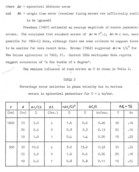
[image:47.553.42.527.52.655.2]

The maximum influence of such errors on C is shown in Table 2.

TABLE 2

Percentage error estimates in phase velocity due to various

errors in epicentral parameters for C =

4

km/sec.

r

d

z

liC t 6 t neSt/CtL (km) (km) / '

(Sec.) e /, km/sec. T dc

1000 50 5.0 4 1.6 6.6 0.26 50 .18

25 2.5 2 0.8 3.3 0.13 25 .10

10 1.0 1 0.4 1.4 0.06 10 .03

500 50 10.0 4 3.2 13.2 0.53 50 .35

25 5.0 2 1.6 6.6 0.26 25 .18

10 2.0 1 0.8 2.8 0.11 10 .03

The temporary recording stations used in this study did not

contri-bute data for the epicentre solutions used, and so I have assumed that errors

in these solutions are not correlated with the azimuths of source to station

paths.

,

Having regard to sign, standard errors of, say, T and o

4

seconds in

(48)

about 1/80 in path length and zero seconds in travel time. Paths with azi

-muths in quadrants containing, or opposite to, the displaced epicentre will

vary accordingly, while those in the remaining two quadrants will be little

affected. It is also asumed that errors in origin time will be equally

distributed as regards sigh.

On the above basis and using the figures given in Table 2, I take

= 10 km and At = 1 second as appropriate "average" errors in epicentre

and origin time, and expect accumulated corresponding errors in phase velocity

of about 0.06 km/sec. and 0.11 km/sec. for path lengths of 1000 and 500 km

respectively.

Separation of profiles corresponding to 40 . =.4rA •are given in the

last column of Table 2. These exceed the "average" errors of .06 and .11 by

a factor of 2 for periods longer than about 30 sec. Hence identification of

separate profile groups should therefore be possible in this longer period •

range.

Larger average errors in r and t would produce an obvious "smearing"

of groups of profiles for events having paths of about the same length. This

should be normally evident for periods below 30 sec. or so, a limit which

therefore depends on the errors in a particular set of observations.

(b) Shape of Profiles

Families of such "single station curves" (section 2.2.2) will

exhibit two kinds of scatter

(a) due to errors Ar and At

(b) .due to errors in

0,,

where this is assumed to be inTria

Errors of type (a) will cause displacement of the dispersion curve by an

amount AC which depends on C rather than T. For example, using model 117,

Appendix 2 as a guide, C varies between

3.4

and 4.0 km/sec. in the T range

20 to 50 sec. If ACVC = 3%, AC varies from .12 to only .10 over this T

range i.e. an almost parallel displacement. Errors of type (b) are

(49)

Thus families of single station profiles will be scattered rather than coherently grouped if errors of type (a) are significant. Such scatter-ing is distscatter-inguishable in the profile shape, from the uniform spreadscatter-ing of profiles which occurs if type (b) exist.

2.3.2 Variation of Initial Phase with Period

Although the frequency dependence of A, influences both group and phase velocities, it has not so far been taken into account in studies of either because too little is klaown about the nature of earthquake source ,-parameters. Most investigations have been content to assume an impulse type

source or a displacement step. Recently Knopoff and Schwab (1967) deduced some relations between frequency and initial phase assuming a line source at an inclination of 450,and a particular geometrical waveguide configuration. For fundamental mode Rayleigh waves, they found that

1 = (.0832T - 2.07)/r C C

. where C = correct phase velocity (r =00), in km/sec. = measured phase velocity

r = epicentral distance, in km T = period, in seconds

(50)

•