CRUSTAL STRUCTURE STUDIES IN TASMANIA
B.D. JOHNSON, M.Sc. (Durham)
Submitted in partial fulfilment of the requirements for the Degree of
Doctor of Philosophy
UNIVERSITY OF TASMANIA HOBART
ABSTRACT
A regional gravity survey of Tasmania has revealed that the crust is of normal continental thickness (35 to 40 kms), increasing slightly under the Central Plateau region and thinning rapidly at the continental margin. The "regional" field, due to the variation in crustal thickness, has been obtained by approximating the observed data, using a
terminated Fourier series; the trigonometric functions having been orthogonalised, with respect to the irregularly spaced data points, by the Gram-Schmidt method.
A time-term analysis of the Bass Strait crustal
refraction data indicates near normal thicknesses in Tasmania and intermediate thicknesses in Bass Strait (23-28 kms).
This thesis contains no material which has been accepted for the award of any other degree or diploma in any
University and, to the best of my knowledge and belief, contains no copy or paraphrase of material previously published or written by another person, except where due reference is made in the text of this thesis.
"Far over the misty mountains cold
To dungeons deep and caverns old
We must away, ere break of day,
To find our long-forgotten gold.
from The Dwarves Song, in
0.00
TABLE OF CONTENTS
Table of Contents List of Figures List of Tables 1.0 INTRODUCTION
1.1 Outline of Physiography and Geology of Tasmania 1.2 Aims of Present Study
2.0 REGIONAL GRAVITY SURVEY OF TASMANIA 2.1 Historical Development of Survey
2.1.1 Initiation of Survey
2.1.2 Early Surveys (1960-1965) 2.1.3 Isogal Survey
2.1.4 Survey of Eastern Tasmania
2.1.5 Survey of North-Eastern Tasmania 2.1.6 West Coast Survey
2.1.7 More Recent Surveys (1968-1970) 2.2 Survey Methods
2.2.1 Instrumentation
2.2.1.1 Gravity Meters 2.2.1.2 Microbarometers 2.2.2 Survey Techniques
2.2.2.1 Drift Control
2.2.2.2 Adjustment of Intervals
0.01
Page 2.2.2.3 Reduction of Gravity Data 2.10 2.2.2.4 Location of Gravity Stations 2.12 2.2.2.5 Accuracy of Gravity Values 2.12
2.2.3 Data Files 2.15
2.2.3.1 University of Tasmania File 2.15
2.2.3.2 B.M.R. Files 2.15
2.3 Bouguer Anomaly Map of Tasmania 2.16
3.0 ANALYSIS OF GRAVITY DATA 3.00
3.1 Determination of Regional Field 2.01
3.1.1 Averaged Data Set 3.02
3.1.2 Choice of Interpolation Method 3.04 3.1.3 Gram Schmidt Orthogonalisation 3.05
3.1.4 Orthogonality 3.08
3.1.5 Analysis of Averaged Data Set 3.11 3.1.5.1 Computational Restrictions 3.11 3.1.5.2 Co-ordinate Transformations 3.14 3.1.5.3 Terminating the Approximations 3.15 3.1.5.4 Boundary Problems 3.16 3.1.5.5 Analysis of Average Bouguer
Gravity 3.16
3.1.5.6 Behaviour of Residuals 3.18
3.1.6 Regional Gravity Map 3.19
0.03
Page
4.1.1.1 The Mt. Field Gravity High 4.02 4.1.1.2 The Great Lake Anomaly 4.03 4.1.1.3 Dolerite Structure in the
Hobart Region 4.04
4.1.1.4 The Lake Leake Gravity High 4.05 4.1.1.5 General Comments on Dolerite
Structures 4.05
4.1.2 Anomalies Associated with Ultrabasic
Bodies 4.06
4.1.2.1 Ultrabasic Bodies with no
Gravity Expression 4.06 4.1.2.2 Bald Hill Ultramafix Complex 4.07 4.1.2.3 Macquarie Harbour Ultrabasics 4.08 4.1.3 Anomalies Associated with Granite Bodies 4.08 4.1.3.1 The North-East Granite Anomaly 4.08 4.1.3.2 The Cox's Bight Granite Anomaly 4.09 4.1.3.3 The Heemskirk Granite Anomaly 4.10 4.1.3.4 The Meredith Granite Anomaly 4.10 4.1.4 Anomalies Associated with Graben Structures 4.10 4.2 Interpretation of the Regional Field 4.11
4.2.1 Choice of Isostatic Model 4.11 4.2.2 Calculation of Isostatic Model 4.13 4.2.3 Comparison of Isostatic Model with
regional anomaly 4.13
0.04
Page
4.2.3.4 Line 800000 North 4.16 4.2.3.5 Line 850000 North 4.16 4.2.3.6 Line 900000 North 4.17 4.2.3.7 General Comments on Interpretation
of Isostatic Model Profiles 4.17 5.0 ANALYSIS OF BASS STRAIT UPPER MANTLE CRUSTAL
REFRACTION EXPERIMENT 5.00
5.1 The Bass Strait Upper Mantle Project (BUMP) 5.01 5.2 Time Term Analysis of Bump Data 5.01
5.2.1 The Time Term Method 5.01
5.2.2 Calculation of Crustal Thickness 5.03 5.2.3 Results of the Analysis 5.04 5.2.4 General Comments on the Bump Results 5.05 6.0 SPECTRAL ANALYSIS OF AEROMAGNETIC PROFILES 6.00
6.1 Previous Work 6.01
6.2 The Depth Determination Technique 6.04 6.2.1 The Upward Continuation Filter 6.04
6.2.2 The Source Spectrum 6.05
0.05
Page
6.3 The High Level Aeromagnetic Survey of Tasmania 6.11
5.4 Data Preparation 6.12
6.4.1 Translation of Data Tapes 6.12
6.4.2 Preliminary Smoothing of the Data 6.13
6.4.3 Data Files 6.14
6.5 Depth Analysis of Tasline 8W 6.14
6.5.1 Spectral Analysis 6.14
6.5.2 Section 1 6.15
6.5.3 Section 2 6.16
6.5.4 Section 3 6.16
6.5.5 Section 4 6.17
6.5.6 General Comments on the Depth
Interpretation 6.17
7.0 CONCLUSIONS 7.00
7.1 Conclusions 7.01
7.2 Acknowledgements 7.02
REFERENCES R.01
Appended Reprint
Johnson, B.D., (1971), Convolution Filters at
ends of Data Sets: Bull. Aus. Soc. Expl.
Geophysicists 2, 11-24,
Appendix
Bouguer Anomaly Map of Tasmania
0.06
LIST OF FIGURES Page
1.1 Topography of Tasmania 1.04
1.2 Geology of Tasmania 1.04
2.1 Isogal Gravity Station Network in Tasmania 2.02
2.2 Major Sources of Data for Regional Gravity
Survey of Tasmania 2.06
3.1 Distribution of Averaged Data Set 3.04
3.2 Map of Averaged Data Unsmoothed 3.04
3.3 Filtered to 20 kms 3.04
3.4 Filtered to 40 kms 3.04
3.5 Ordering of Fourier Coefficients 3.06
3.6 Distribution of Artificial Data Sets
(a) Regular 3.08
(b) Random 3.08
3.7 Flow Sheet of Gram Schmidt Analysis 3.13
3.8 Analysis of Unfiltered Data Synthesised to K=3 3.17
3.9 Synthesised to Y=4 3.17
3.19 Analysis of Data Filtered to 20 Kms
Synthesised to K=3 3.17
3.11 Analysis of Data Filtered to 20 Kms
Synthesised to K=4 3.17
3.12 Analysis of Data Filtered to 40 Kms
Synthesised to K=3 3.17
3.13 Analysis of Data Filtered to 40 Kms
Synthesised to K=4 3.17
3.14 Comparison of Variance of Residuals with
Additional Wavenumber for each Data Set 3.18
3.15 Regional Gravity Map with Locations of Averaged
0.07
Page
4.1 Elements of Residual Bouguer Anomaly Map 4.01
4.2 Gravity Map of Mt. Field Anomaly 4.02
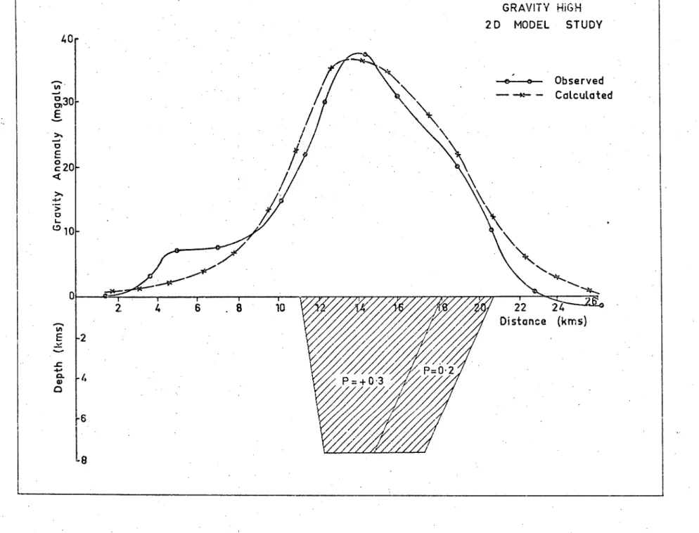
4.3 Two Dimensional Model Analysis of Mt. Field
Anomaly 4.03
4.4 Bald Hill Complex, Two Dimensional Model
Analysis 4.07
4.5 Isostatic Model System 4.12
4.6 Isostatic Model Gravity Field
Standard Crust = 30 Kms 4.13
4.7 Isostatic Model Gravity Field
Standard Crust = 35 Kms 4.13
4.8
to Isostetic Model Gravity Profiles 4. 1 4
R,13
5.1 Location Map of Shot Points and Receiving
Stations 5.01
5.2 Time Term Analysis of Bump Data 5.04
6. 1 Total Magnetic Intensity Profile Map of Tasmania
6.2 Tasline 8W Location Map
6.3 Spectrum of Section 1 of Tasline 8W
6.4 Spectrum of Section 2 of Tasline 8W
6.5 Spectrum of Section 3 of Tasline 8W
6.6 Spectrum of Section 4 of Tasline 8W
6.12
6.15
6.15
6.15
6.15
0.08
LIST OF TABLES Page
3.1 Averaged Data Set
(a) Unsmoothed
(b) Filtered to 20 Kms
(c) Filtered to 40 Kms
3.2 Function Set for Gram-Schmidt Orthogonalisation
3.3 Gram Determinant Calculations
3.4 Total Number of Functions Against Wavenumber
3.5 Coefficients of Analysis of Unfiltered Data
3.6 Coefficients of Analysis of Data Filtered
to 20 Kms
3.7 Coefficients of Analysis of Data Filtered
to 40 Kms
3.03
3.03
3.03
3.06
3.10
3.11
3.18
3.18
CHAPTER ONE
1 .01
1.1 OUTLINE OF PHYSIOGRAPHY AND GEOLOGY OF TASMANIA
Tasmania is the southern most portion of the continental
land mass of Australia. Although it is an island, it is
connected to the mainland by Bass Strait, which is of typical
continental shelf depths (< 100 m).
To the east and west of Tasmania there is a narrow
continental shelf with a steep continental slope. Normal
oceanic depths (> 2000 m) are thus encountered within a
distance of only 40-50 kms of the coastline. To the south
there is a southward extension of the bathymetric contours.
This feature consists of a deep ridge or rise, known as the
South Tasmanian Rise with depths of the order of 1000 m.
Very little is known about this structure.
Tasmania is therefore relatively unique in that it
approaches being a continental land mass of very small aerial
extent. In particular, an east-west profile taken across the
island, consisting of an oceanic-continental-oceanic section,
has a total length of only 5-600 kms.
The topography of Tasmania is dominated by the
geological structure which often gives rise to spectacular
land forms. In the north-eastern part of Tasmania, there is
a high mountainous region with peaks at Ben Lomond (over
1600 m) and Mt. Barrow (1500 m). These peaks are situated on
a granite mass which is exposed over a large part of the
1.02
To the west, there is a low lying area dominated by the north-west trending Tamar valley. This is a graben feature of Tertiary age and is filled with Tertiary and more recent sediments.
To the south and west of the Tamar valley, there is a steep rise to the Central Plateau region. Near-vertical cliffs, or tiers, are formed at the edge of the plateau due to the exposure of sills of dolerite. The elevation of the Central Plateau region is around 1000 m reaching up to 1400 m at the north-eastern margin.
In the south-east, the dolerite forms a partial cover over a large portion of the area. The sediments and volcanic rocks in this region are relatively young being mainly Permian or younger. The topography is largely dominated by the local structure of the dolerite.
To the west and south of the Central Plateau, the
terrain becomes much more rugged, partly due to the formation of deeply incised river valleys. The highest peaks in
Tasmania are found in the area west of the Central Plateau (Mt. Ossa, 1700 m). Toward the south the mountains form distinct regions separated by deep river valleys. These mountains (Mt. Field West, Mt. Styx, Mt. Wellington, the Hartz mountains and Mt. La Perouse) form a chain of
mountains extending to the south coast. The peaks are of the order of 1300 m rising from a plateau level of the order
1.03
In the remote south-western part of the state the
mountains form long gently arcuate ridges, mainly composed of quartzite or metamorphosed sediments of Palaeozoic age or older. The regions between the ridges are flat low-lying swamps (one of the few regions of the state where the normally dense tree cover is not so marked).
The drainage pattern of Tasmania has been examined (e.g. Davis, 1959) and there are several interesting features. The drainage divide, between river systems, commonly occurs near the coast line. This is most clearly demonstrated on the east coast where the divide is within a few miles of the sea. The Derwent valley and its estuary has a typical drowned
river valley appearance. This combined with the unusual
drainage patterns indicate that the south-eastern part of the state has suffered subsidence during the Pleistocene
(Jennings, 1959).
This very brief outline of Tasmania has been drawn from two major sources: the Atlas of Tasmania (Davis, 1965), and the Geology of Tasmania (Spry and Banks, 1962). Maps of the topography and geology of Tasmania are included as Figures 1.1 and 1.2, respectively. For the further background
information the reader is referred to these two texts.
1.2 AIMS OF THIS STUDY
In order to properly fulfil this aim a number of secondary aims were detailed.
1. The establishment of a regional gravity survey over the whole state,
2. The development of techniques to separate the regional and residual components of the gravity field.
3. The choice of a suitable coefficient set such that the regional field could be evaluated in any part of the state.
4. The interpretation of the gravity data in terms of the crust-mantle interface and major upper crustal structures.
5. An independant estimate of the crustal thickness indicated by crustal seismic refraction data.
6. An examination of the spectral properties of high level aeromagnetic data to ascertain whether or not
information on deep crustal structure could be found. In brief, the problem, to obtain information on the
FIGURE 1.1
14t 140
45
BA SS STR AI T
Feet 405
50X
4000
3000 20X WOO
Id
4
Hunter Idit Robbsns Id
Fathoms
Stralt
Banks
42
s,4.ou,.4 Id
43
60 )15 a
r 50
,0 5 0 low -- ,
'--;-.5....
N'"'""
P7,00.4.
FIGURE 1 . 2
145.
BASS STRAIT
111,
three hlwrinvock IdHunter Id
C. G/00 Robbins Id.
C °"47—'\--\ Ja
T. Cep.
Sandy Cope
C Sonll
STRATIFIED ROCKS el,
KRUM D4IR$111111 ORDCMCIA0 110
—j
PIKCA111111101 Ilmserneoul MCMINN 0111msasusl
Mario Id
Lew Rocky h
*MOUS 1003
11. RAMAT MAI ASA= - aiTACIOUS Spomb
11111 SUVA= NW%
•
•
•
000011111 (Wile
CIPAIMIA/I Gramb
•Tosmon Id
Port Davey
SW Cope
oweetsuvie,
so Cop.
/0 II II 01 10 Min
-r
Pro/00m Noon. 110a001
CHAPTER TWO
2.01
2.1 HISTORICAL DEVELOPMENT OF SURVEY
2.1.1 Initiation of survey
The regional gravity survey of Tasmania was initiated in 1960 by R. Green, then Senior Lecturer in geophysics at the University of Tasmania. In the initial phases of the gravity survey students carried out local exercises of very varying quality. Some of this work has been retained.
2.1.2 Early surveys (1960-1965)
A number of surveys of particular regions were carried out by Honours students in the period 1960-1965.
McDougall and Stott (1961) carried out an investigation of the Red Hill Dyke, near Margate. Shelley (1965) surveyed an area in the vicinity of Sorell and Leaman (1965) carried out a geological and geophysical investigation of the Cygnet Complex. These surveys were all of very restricted areas.
Larger scale surveys were carried out by Jones (1963); (Jones, Haigh and Green (1966)), who investigated the
structural form of the Great Lake dolerite body, and by Hinch (1965), who surveyed the Cressy region near Launceston and interpreted the observed gravity low as a Tertiary sediment filled graben.
2.1.3 Isogal survey
2.02
Australia. The purpose of that survey was to establish
permanent gravity base stations along east-west lines across the Australian continent. The resulting measurements made by several independent gravity meters have been adjusted by
least squares techniques and have achieved a national network of base stations that are considered accurate to ±0.1 mgals. • (Barlow, B.C., in preparation).
The datum base for this survey is the Australian
National Gravity Base Station in Melbourne, which is taken to have a value of 979.979 gals. (Barlow, B.C., 1970).
Some of the isogal stations have been used, in Tasmania, as a basis for adjustment of all the gravity surveys that have been carried out to date. These are Hobart (airport), Hobart, Launceston, St. Helens, Wynyard and Strahan. Each
survey has therefore been made internally consistent and has also been adjusted so that the observed intervals correspond to those obtained during the isogal survey.
Figure 2.1 shows the locations and values obtained for the Tasmanian isogal stations.
2.1.4 Survey of Eastern Tasmania
During 1966, B.F. Cameron, carried out a compilation of existing surveys and completed the regional gravity survey of eastern Tasmania. (Cameron, 1967).
BUREAU OF MINERAL RESOURCES GRAVITY BASE STATIONS IN TASMANIA
0
SMITHTON 6491.1142 980.27498
DEVON PORT 6491.1141 980.28209
ST HELENS 6491.9139 980.30229
LAUNCESTON 6850.0171
980.27546
STRAHAN 6491.9136 980.37169
HOBART
(AIRPORT)
6491.0160 980448.91 HOBART
(UNI )
6091.0160 980.44427
2.03
involved recomputation and adjustment of survey parameters. The original gravity reduction programme (U191, written by R. Green) was modified for this recomputation.
The second part of the project was to take gravity measurements in selected regions of eastern Tasmania. This was intended to provide a more complete coverage of the
region and to tie together the previously unrelated surveys. The result of this work was the establishment of a
gravity survey, on a regional scale, which covered most of the eastern part of the state. The survey was confined to regions accessible by vehicular transport. Some interesting anomalies were identified and preliminary interpretations were carried out.
Cameron was able to define a regional gradient, in the Bouguer anomaly, which varies from +20 mgals at the east coast to -40 mgals in the Central Highlands area. This was interpreted as being due to crustal thickening towards the centre of Tasmania from 34 kms to about 39 kms.
2.04
A large negative feature was identified on the northern margin of the area, near Avoca, which was interpreted as being due to either a granite body or a sedimentary feature. The remaining features of the gravity field were interpreted
in terms of dolerite structures.
The thesis was completed by a useful list of
recommendations for future surveys. This list was referred to in planning the subsequent stages of the regional gravity survey of Tasmania.
2.1.5 Survey of North-eastern Tasmania
Following the work of Cameron (1967) several additional surveys were undertaken in order to extend the coverage of the regional survey. A survey of the north-eastern part of the state was carried out by Cameron in order to establish the extent of the Avoca gravity low. The survey was
restricted to road traverses as the terrain is very rugged. The survey was able to delineate the shape of the
gravity feature. The gravity low observed on the Avoca traverse is seen to extend northwards and coincides
2.05
2.1.6 West Coast survey
During 1967, a survey of the West Coast region of Tasmania was carried out by myself with the assistance of B.F. Cameron and M.J. Rubenach. (Johnson, B.D., 1967).
This consisted of road traverses along the Lyell, Zeehan and Murchison Highways. Much of this region is extremely inaccessible except along these roads.
The survey was then extended into the north-western part of the state along the Savage River road and along the north coast.
A further road traverse was carried out along the Gordon River road leading to the new Gordon River damsite in the South West of Tasmania. A number of short traverses were also made in the National Park region along timber tracks.
The coverage thus obtained was therefore almost complete for all road access. A successful approach was made to the Broken Hill Co. Pty. Ltd. to assist the survey by making some helicopter time available. This enabled the establishment of over 200 gravity stations reasonably uniformly distributed throughout this otherwise inaccessible region of the state.
The regional survey has been carried out on the basis of availability. Much of the terrain that remains to be
2.06
2.1.7 More recent surveys (1968-1970)
Further surveys have been carried out, since 1968, by several authors, in order to define particular geological problems.
A survey of King Island (to the north west of Tasmania) was carried out by myself and G.M. Sheehan. The survey was interesting in that a reasonably uniform station coverage of the island was possible and that the geological structure was largely hidden due to recent sand cover.
A survey of the Sheffield region of northern Tasmania was carried out by G.M. Sheehan (1969).
Further work was carried out in the Longford-Cressy region by M.J. Longman of the Mines Department, Hobart
(Longman Leaman, 1967) which greatly extended the work of Hinch (1965). A major reinterpretation of this work has subsequently been carried out.
A detailed study of the dolerite distribution and structure, in the Hobart district, was undertaken by D.E. Leaman (1970).
2.07
2.2 SURVEY METHODS
2.2.1 Instrumentation
2.2.1.1 Gravity meters
A number of gravity meters have been used during the period of the gravity survey of Tasmania. The main
instrument was the Warden No. 273 of the Geology Department, University of Tasmania. This was originally purchased in 1960 and had an 80 mgal range dial on the fine adjustment spring. During 1967, the instrument was returned to Texas Instruments and fitted with a new 200 mgal range dial. This greatly improved the performance of the instrument since only occasional scale changes were required during the course of a survey.
During the absence of this instrument, the Warden Master No. 201 of the Geophysics Department, Australian National University was borrowed. This instrument was used only in restricted areas as it was found to have a relatively high drift rate.
The helicopter survey of the south western area of the State was made with a portable La Coste-Romberg meter, G101, on loan from the Bureau of Mineral Resources, Canberra. The instrument was chosen for its supposedly excellent drift characteristics. However, in subsequent surveys
2.08
pers. comm.). It is possible that some errors have therefore been incorporated into the survey values. Drift rates were observed during the survey but these were regarded as not being serious, in view of the errors in position and
elevation.
202.1.2 Microbarometers
Two types of microbarometers were used to establish levels for survey stations. The first, Askania
microbarometers, were found to be very sensitive to wind
conditions, difficult to operate over large elevation changes and were not really accurate enough for this kind of survey. The second, Mechanism microbarometers, were found to be
reliable, easy to use and sufficiently accurate for regional surveys. All the earlier surveys were carried out using the Askania microbarometers. Certain difficulties arose due to the lack of precision of these instruments, but this could be overcome in part by surveying around the contour and between fixed level points as far as possible (Longman, M.J., pers. comm.). It is considered that the errors in the elevations are the major source of error in these surveys.
2.2.2 Survey Techniques
2.2.2.1 Drift Control
2.09
the gravimeter spring.
It has been found that it is sufficient to assume linear variation of the spring in periods of the order of 1 hour. In order to account for this, repeated readings must
therefore be taken at a number of the stations, the time interval being not much greater than 1 hour.
Since we are interested only in the relative differences between stations (even with a meter having a world wide
range), it should only be used in the relative mode. It is a straightforward matter to determine the drift corrected
gravity intervals. It is important, however, to establish a clearly defined routine method; since without this it is difficult for different people to arrive at the same answers.
Since, in all of these surveys, microbarometers were used to obtain levels, it was found convenient to reduce the barometric values in the same manner as the gravity values. In this case the pressure is varying with time and not the measuring device. Again the barometer was used in a relative sense between fixed levels, normally state permanent marks.
This process can be automated as in the Bureau of Mineral Resources System of reduction of gravity data
(Barlow B.C., Pers. Comm.).
2.2.2.2 Adjustment of Intervals
2.10
In the eastern part of the state complex loop patterns were adjusted by standard least squares methods (e.g. see Cameron, B.F., 1967).
In the remainder of the state, most of the surveys were carried out between two isogal stations or were tied to only one of these stations. In the former case simple linear adjustment was carried out for the survey values. This was considered to be completely adequate as the largest
misclosures obtained during the regional survey were 0.05 mgals. This is within the accurace of the isogal values.
The helicopter survey of the south west of Tasmania was directly connected to the isogal station at Strahan airport. As a check, connections were made at Port Davey, where a temporary base station had been established by air from Sydney, and at the Gordon River Road. Both of these observations tied in well considering the measured drift variation in the La Coste-Romberg instrument. (The
differences in the observations were 0.15 mgals at Port Davey and 0.06 mgals at the Gordon River Road.)
2.2.2.3 Reduction of Gravity Data
2.11
The base station value and survey parameters are
initially read in. Each station is then treated separately and the following sequence of operations is carried out:
1. multiplication of scale readings by the calibration constant of the meter.
2. adjustment of gravity intervals (if applicable) 3. addition of base station value
thus giving absolute values of the observed gravity at each station
4. calculation of theoretical gravity from International Gravity formula
(g() = 978049.0 (1 + 0.0052884 sin 2 (I) - 0.0000059 sin 2 2) mgals where (I) is latitude of station 5. calculation of free air anomaly
gA = gh + 0.3086 h - g(0 mgals gA = free air anomaly
gh = gravity at height h meters 6. Calculation of Bouguer anomaly
g B = g A - 0.04185 o h mgals g B = Bouguer gravity anomaly
o = density (normally use 2.67 gins/cc) 7. print out consisting of:
station number, position, elevation, theoretical gravity (4), observed gravity (3), free air anomaly
2.12
2.2.2.4 Location of gravity stations
The gravity stations were located by means of
topographic survey maps and in some cases air photographs. The quality of the positioning is very variable since the accuracy of the topographic surveys is extremely variable.
Cards giving the description of the location of most of the gravity stations are lodged with the Geology Department, University of Tasmania.
2.2.2.5 Accuracy of gravity values
The accuracy of the gravity values is a function of a number of different factors:
Calibration constant of the meter
All the instruments used in this survey were calibrated on the Hobart calibration range (Barlow, B.C., 1967).
Although some doubt has recently been raised over the actual value of the gravity interval of the Hobart range (Barlow B.C., pers. comm.) this has been assumed to be not serious.
Errors of the order of 0.01 mgals may be attributable to errors in the calibration constant.
Latitude of the gravity station
Errors in the positioning, and in particular, the
2.13
Thus an error in positioning may be directly related to errors in the gravity value.
Expected error in Error in
Positioning (km) Gravity (mgals)
0.01 - 0.008
0.1 0.081
1 0.807
Errors in positioning are generally better than 0.1 kms for the eastern parts of the state and for areas that have been mapped for the Hydro Electric Commission. Other areas in the South-west of the state and in other poorly mapped areas may well be in error by greater than 0.1 kms but are certainly better than 1 kms.
Errors in elevation
Errors in elevation of the gravity station often lead to the most serious errors in the Bouguer anomaly values.
The combined elevation correction (using a density of 2.67 gms/cc in the Bouguer correction) is 0.1967 mgals/m. Thus an error of 1 meter in elevation gives rise to an error of 0.2 mgals.
2.14
Effect of Terrain Correction
The work of St. John (1967), and St. John and Green (1967) has shown that topographic corrections should be
rigorously applied in regions of rugged terrain, taking into account the curvature of the earth, the departure of the topography from the Bouguer approximation and effects of horizontal variations in density.
In general there are two distinct regions of influence affecting the terrain correction at a given point. The first part is due to extremely local terrain variations; where only spectacular topographic variations, within a distance of less than a kilometre or so, have any appreciable effect. The second part is due to the inadequacies of the normal
topographic correction process. This second effect must vary very slowly from station to station as the masses causing the effect are at a cnnsiderable distance from the station. The effect is only serious for high mountainous regions, such as New Guinea, which are closely associated with deep oceanic regions.
This second source of topographic correction has been ignored in this work, any large scale topographic variations being included in the isostatic model developed in the
2.15
The Bouguer Anomaly values are therefore considered accurate to ±0.2 mgals in all regions and are generally accurate to ±0.5 mgals.
2.2.3 Data Files
2.2.3.1 University of Tasmania File
A file of the original field data and reduced data for all the surveys is held at the Department of Geology,
University of Tasmania.
A system for collating the results of the reduction
programme was initiated in 1968, by myself. This system uses the programme, U606 GRAVDECK, which takes the reduced data tapes from U191 and combines these values with those present in the tape files. Facilities exist for deleting, exchanging and overwriting surveys or individual stations. These paper tape files are also lodged at the University of Tasmania.
2.2.3.2 B.M.R. Files
The Bureau of Mineral Resources, Canberra, has for several years been carrying out a systematic gravity survey of mainland Australia. Some of this data has been placed on computer files and may be readily accessed.
2.16
2.3 BOUGUER ANOMALY MAP OF TASMANIA
The results of all gravity surveys carried out during the period 1960-1970 have been compiled using a crustal
density of 2.67 gms/cc and a Bouguer anomaly map of Tasmania has been drawn. Considerable assistance with this project was generously given by Mr. B.F. Cameron. A copy of this map at 1:500,000 scale is placed in the appendix to the thesis.
CHAPTER THREE
3.01
3.0 ANALYSIS OF GRAVITY DATA
Before any meaningful interpretation can be made of the Bouguer anomalies, observed in Tasmania, consideration must be given as to the source of the anomalies.
The most striking feature of the Bouguer anomaly map is the regional effect due to the close proximity of the oceanic crustal structure. This causes the values, near to the coasts, to have a steep positive gradient of the order of 1 mgal/km toward the ocean.
Superimposed on this regional anomaly are many smaller scale anomalies that are due to structures which are
shallower than the depth of the continental crust.
In order to separate these smaller scale anomalies from the broader regional anomalies, an effective method must be found in order to adequately represent the regional component. Once this has been carried out the regional component may be removed from the observed values to give the residual anomaly due entirely to shallow sources.
3.1 DETERMINATION OF REGIONAL FIELD
The complete set of the gravity data is extremely unevenly distributed. Surveys have been carried out in detail in restricted regions, along roads and vehicular tracks, and in isolated positions accessible only by helicopter.
3.02
spaced data, is biased towards fitting the surface to the data points. Hence, if we have a restricted region of complex data, and a large proportion of the data set is
present in this region, then the surface in the area adjacent to the detailed region will also tend to reflect the complex nature of that region. The effect is thus to produce a
highly complex surface in an area where there are few, if any, data points.
It is necessary therefore to remove this bias from the data set. This was carried out by averaging the original data set and producing a subset of more evenly spaced and smoothed data.
3.1.1 Averaged data set
The method chosen to obtain a smoothed subset of the data was by a form of convolution filtering.
The average value and position was calculated for all stations lying within each 20,000 yard (approx. 20 kms) grid square. This procedure was chosen to limit the amount of computer calculations involved. In any process of aerial smoothing, distances are normally calculated between every possible pair of data points. If the number of points, n, is large, then this can become prohibitive since there are of the order of n 2 calculations.
3.03
known in terms of the Transverse Mercator grid coordinates giving distances in yards north and east from a fixed point. A station can be defined to lie within a particular 20,000 yard square by carrying out an integral division of the coordinates by 20,000. It is then a simple matter to
reference all the stations within a particular square, and to carry out averages of value and position. The number of
calculations has been reduced to order n.
However this is not the end of the process since the averaging of the data set has introduced spurious effects into the data. The averaging process is approximately
equivalent to the application of a two-dimensional sin xf/xf filter in frequency. The data must be further smoothed to eliminate the deleterious effects of the simple averaging process.
A second stage of filtering was therefore carried out on the averaged data set. The process chosen for this stage was to perform a convolution by averaging all the values within a distance, r, of each station. This is equivalent to
applying a sin rf/rf filter in frequency. To reduce the effect of the side lobes, the process was repeated. The effects of repeated application of a convolution filter are well demonstrated in Bracewell (1965, p171).
T S• 9 GS' CZ
66' hZI 6 hL•T-
3L•2 Z9•62
1 hL° T-
0 L• Z 2 9* 62
I 000b62 CGE60L 90L
52 91 2 L' tr.?. hi.' SL 9 21'62 6 h'62
92 '2 ' 2 02' 82
62' 9: 9 h• Z 02 9L
92 Oh T90L 950 L
7.7.' ZZ
• 99' 87.
1 IVY.; 9 • 08.'02 22°12 69'h Z 9T' 9£ 92' 92 L3' OT I 032992 30620L hECL • 3Z•82 99" ££ ZO•Oh h IT'Zi 60•L£ CS •h h
h h 8* h:::
-I 9• 25 0 0' Ot;
6 hhSt:99
629369 363 3
T fi• 9Z. 16° 12 116f7 L h3•Z2 £382 I1*9+2 2 9693
L 2' Lh
T tt• 90T 9 699995 939869 b96'9 Br t2 I2.• LZ 9029 8 £9'.I2 2i.°82 9909 E 28" 92 ZS' 92 00' Z 016129 393929
296 9 .
1 h• ST 52' 92 h8' SL 6 59'91 92°92 L898 h 2 2• LT
6t82 LZ• L9T Z L
hT 2605 029969 0933
9L• 6 98' 9Z 69•ShT 6 3.1•21 2622 'hL•L9 h 90' fit 62" 2Z. "
9 Z.' hi. 19I +76 ri. 6 h
h0 0939
et78 9 DE. e 90 fiee3Lb 6Z' SOT.. G 2 1' L2 TZ' e) . £ 30°0S1 Z2'2:: th'9 Ii.'STZ 8 82'92 SW' t., ,89
L 2" 2-
5 I' 62. IL" ISZ 8
9201- OT•8L 9
.
9 '0 EL 2
L I' bT - 8 8' 6h
h tl' ZL 9 Z 000Lht 032969
+39
LZ• h-
Z3' Z7. 96" h2Z 9
2T'ZI-
L L- 9,
h6•991 h I £• T2- 28"
2E' LGT Z 3S92
096E69 26 9
tiZ•
-
h .1." i.T 99391 6 hZ•f71.- 18'2 h2• 1 :9T Z 91°21- 03' LL 891 Z 08930h 309069 3h2 9 3801 2 6' 91
Z t, ° 19
L
EZ°hZ 99' hZ
6Z5 2 6 L • 22
t; 9 - Z2 9$f Z
809382 002329 9293
IL' 9-1 hi.• TZ 98'59 9 LS '9Z L8'92 69°Z 2 8 T• 9Z
Z2' 9Z - 8E'
.
1 03E91.2 309260 9295
62• ZZ
ST" LZ • h h" 2h
9 9122 ZS"92 S3°92 2 99' La' 9 9' L2
00' I 092029 OZSSL9 2699 .
L).' 91 ES' SZ 99'29 B 95'02 ZZ'hZ ES '172 t7 hO• TZ 0 h•SZ DO' 62 9 . LhI609
SL 02L9 3939
O 0' ET
ZS'LZ
8 I° SZ T 6
6L
21 10•22
hi) 'Z. 8 S 6L• ZT
20° 91 16°61
9 8LL68h 03L31.3 9h99
39°. 22" 02 9120Z a ' 966 Zi"h2 Th•9ZT f7 60' c 36' 32 2 V 02£ 5 OLZLLb
ShSZ L9 990
20' 2 IZ• CZ
ES• ShE 6 9201- OT•SL • 99°062.
C 99'9-
£2901 62' 9001 I 09 L9St? OC‘Z£ L9 ht2 9
6 1 ' I
L L° TZ
62' h9T 6 89 'L - 1b°2 - 20'66 Z.9• ii- 81• 9 62' 69 Z .0Z 09Z h 992T /-3 Ztz9 9 ID' 2. 9391
8 h • ST T 8 LO't:-
28' - OL 7. h
0° 1- h3" T-
h9' 2 IL Sh Th
hE 9S 99 3h93
9L• 9 92' ET
6I•Ch • 3 552Z 90 -bZ 2L•h Z 9222 Lb' h.? EL' CT 2 1.9£252 UO2.i. 93 8233 2E' ET
La .,• 11Z • t Z• 16
S 69•TZ 19•2Z TILT Z 6322 6:-." 22 00' T 092939 0329;9 39f 3
9 0- GI L 0' 3Z ti8•Z6 L 19°21 22•23 t2•8L ti . 22° 91 00* 91 h 3' S
ZS 5h8 h ZS IG 99
91:h 3
0 T• ET 2 T• /2
6h* 8Z 1 9
LZ. '"ST 28'0Z 69'8Z 2 69'81 £ L• ST 32 2 • 2h69Lh :::'•LTh9 9hh 3 30°0I 9 h• SZ
88 OhT L hL 'ET L0'61 69°S 2 CCLT
L 2' ST
69' hi • Z
00 hL hf, 3361: h3 tihh 3
6 h• 9 0.5• CZ 8 h'.91:T L TE•LI 20.'81 32. 9 Z. Z2° S1 92°S1 0E' I 00Z72..h
C322 h9 Zhh '2
T Z• h 8 6' hi-.
02'86 S LG'T - Th' 69 'L 1 • Z SL'-
130' - • 0 L' 9
L
98 ET 1 h ObESh3
Obh 3
09' 91 99' hZ
2 T• 8L S hZ*TZ
9t1'02: Z61
2 21' SZ - 61 CZ
9Z
2
26LhLh L31b£3 9172 9
LE' hT 1.3° SC 9266 S 69.'0Z Zb"OZ 6t) '5 £ 39° CZ
h 9' ZZ 0 E• I
006L5h 000922 tit: 5
S INIO d SINIOd
S iNIOd ISV3
1-ild0N
AlVWONV AlVWONV S3813W VIVO 20 A1Vi4ONV AlVWONV S3211314 VIVO JO
AlVWONV AlV W.:NV S3813W VIVO 30 aitNI08003
X3ON I 83C10006 8I V 038J IHOI31-1 ?i3EW(IN 8 3n0n0e .8I V 3383 IH SI 31-1 83 OW
fiN 83 no no e
b IV 338J IHS/3H
e 35 wn ti 0.7.83
38VrICS
VIVO 02831113 SWN Oh VIVO 03831.11J SWN OZ
VIVO 83 831112Nfl
S38VnSS 0180 (S W>1 92) OA 00002 21:11t0 030 V83AV VIVO
REGIONAL, GRAVITY SURVEY OF TASMANIA
DATA AVERAGED OVER 20600 10 (20 KMS) GRID SGUARES
UNFILTERED DATA 20 KMS FILTERED DATA - 40 KMS FILTERED DATA
SDUARE GRID NUM B.E.-.R HEIGHT FREE AIR BOUGUER NUMBER HEIGHT FREE. AIR BOUGUER NUMBER HEIGHT FREE AIR BOUGUER INDEX - COORDINATE OF DATA METRES ANOMALY ANOMALY OF DATA METRES ANOMALY ANOMALY OF DATA METRES ANOMALY. ANOMALY
NORTH EAST POINTS POINTS POINTS
7640 711980 416730 1 232 .5 4 29.79 -2.96 3 281.42 23.74 -7.75 8 239.94 21.57 -5.23 7642 705950 422750 1 281 .5 1 22 .8 1 -8 .7 0 3 243.77' 17.71 -9.57 7 230.59 23.65 -7.75 • 7045 767999 475726 7 76.08 14.98 ' 6.47 3 127.44 20.64 6.33 3 220.94 24.39 -.33 7648 705481 489664 14 55.58 12.56 6.23. 3 38.71 13.97 9.05 9 147.35 21.50 5.01 72E0 712760 514700 105 164.73 31.12 12.68 4 30.02 22.56 13.62 9 89.23 21.59 • 11.61
7052 7131E1 526316 55 3.69 17.18 16.21 3 71.17 2031.' 12.34 • 9 59.77 24.56 17.37 7054 762925 552175 - 2 7.31 29.33 23.01 4 44.50 37.29 32.11 9 51.89 29.36 23.55 7056 709544 566556 9 32.44 34.47 . 36.84 4 43.04 35.29 30.47 5 44.36 31.15 26.13 7234 730728 • 354970 6 134.21 48.38 33.36 3 85.00 33.49 28.98 7 76.48 31.81 23.25 7236 735011 365600 7 146.52 22.22 5.82 3 110.33 25.91 13.56 9 103.46 26.10 13 ,8 5
7 238 733064 394653 5 277.75 25.25 -4.33 1 224.33 21.27 -3.83 9 187.27 22.85 1.90 7240 729946 409007 20 339.46 31.75 -6.23 4 276.69 24.97 -5.92 9 278.76 23.49 -7.70 7242 736688 431299 18 422.80 34.58 -12.73 , ,_ 433.91 32.13 -16.43 8 338.92 25.87 -12.36 7244 732336 454344 23 371 .36 29 .7 7 -11 .7 9 3 341.65 26.19 -12.04 7 313.76 24.28 -10.83 7246 735345 470000 8 258.33 24.11 -4.83 4 240.34 18.30 -8.60 8 230.05 13.69 -6.05
7249 734381 487183 9 124.01 5.02 -3.86 4 139.03 13.50 -7.65 9 162.91 17.20 -1.03 7250 726890 514419 59 15.23 7.74 6.63 4 55.97 19.51 12.12 9 117.96 18.37 5.17 7252 732488 532393 292 37.92 18.73 14.48 4 58.90 19.13 12.54 9 94.22 21.39 11.45 7254 723800 549300 5 48.86 25.33 20.47 3 47.67 24.93 19.65 9 90.35 25.13 17.14 7256 723783 561933 3 54.95 34.26 23.11 42.10 30.71 26.00 6 72.04 27.83 19.77
7432 756370 336955 2 .07 51.33 51.92 4 50.53 41.57 35.91 5 63.04 35.88 28.82 7434 745316 342940 2 .15 52.58 50.56 3 58.65 45.25 . 38.49 8 . 82.88 31.29 22.21 7436 7E6320 371708 • 4 69.96 3.34• -3.88 4 123.13 16.41 2.63 8 117.33 25.40 12.27
7 438 743130 336575 2 104 .0 2 13.72 2.68 3 170.99 17.01 • -2.13 8 224.34 23.82 • -1.29 7'440 74 4760 414520 1 2.19 .4 6 13.40 -11.16 2 230.39 23.94 -7.49 8 341.31 20.54 -11.65
REGIONAL GRAVITY SURVEY OF TASMANIA
DATA AVERAGED OVER 20300 YO (20 KMS)6 GRID SOUARES
SDUARE
INDEX COORDINATE GRID NORTH EAST •
NUMBER OF DATA POINTS
UNFILTERED DATA
HEIGHT FREE AIR
METRES ANOMALY ANOMALY BOUGUER
20
NUMBER OF DATA POINTS
KMS FILTERED DATA
HEIGHT FREE AIR METRES ANOMALY
BOUGUER ANOMALY 40 NUMBER OF DATA POINTS
KMS FILTERED DATA.
HEIGHT FREE AIR BOUGUER METRES ANOMALY ANOMALY
7452 746597 527884 117 99 .5 2 15.98 4.83 3 73.25 14.61 ' 5.85 9 160.92 22.11 4.10 7454 752284 555432 19 137.82 25.27 9.85 2 95.31 21.27 10.61 9 130.67 23.93 • 9.31 7456 7555 35 561463 4 52..31 17.28 11.37. 2 95.31 21.27 10.61 6 111.90 24 .4 4 11 .0 i 7632 774130 335555 2 78 .4 2 49.58 39.30 4 55.15 35.94 30.33 6 78.22 32.10 23.35 7634 773455 351024 12 71.46 27.02 19.32 5 73.57 30.56 32.32 9 135.67 23.37 13.44
7636 7623 33 361.383 2 169.76 13.26 -3.75 3 102.44 13.82 7.35 8 168.23 23.02 4.20 7643 77 60 23 41 55 80 1 331.78 16.37 -20.76 2 634.04 40.16 -27.43 6 410.99 29.61 -15.38 7342 761620 425460 1 876.3C 63.35 -34.11 2 61 4. 04 40.16 -77.43 8 475.19 34.12 -19.35 7544 774068 450011 13 339.37 17.29 -20.74 3 403.42 24.61 -20.19 9 460.12 32.19 -19.29 7646 765519 457967 14 141.26 -3.53 -13.34 3 31 4. "'S 17.31 -17.91 9 398.40 28.02 -16.56
7548 770915 485788 11 354.17 28.74 -10.89 3 330.35 21.73 -15.23 9 340.32 25.57 -12.51 7553 775783 507444 17 265.63 18.05 -11.67 2 351.79 31.45 -7.91 9 304.44 26 .2 2 -7.94 7 652 774108 525750 8 407.2.1. 41.74 -3.33 5 375.37 34.80 -7.20 9 262.13 26 .8 4 -2 .4 9 7654 773375 543333 2 296 .7 2 23.91 -4.25 4 355.30 34.60 -6.23 9 204.64 25 .28 2.33 7656 772653 573358 9 45.90 15.59 13.45 2 29.83 12.61 9.47 7 159.93 23.11 5.21
7332 7893E9 332746 7 2.69 37.63 37.33 65.20 28.31 21.51 6 96.75 24 .6 2 13.79 7634 738094 353079 15 88.33 13.46 3.57 4 103.33 23.73 12.27 9 133.73 22.35 7.33 7336 739210 365310 1 266.15 14.23 -15.58 2 142.23 18.45 2.54 8 213.41 25.29 -3.59 7333 783695 392105 2 345.70 25.33 -13.36 1 345.70 25.33 -13.36 7 332.23 24.52 -12.65 7 242 794189 432413 -15 674 .16 55.93 -19.51 3 841.30 50.12 -21.73 8 579.00 42.95 -21.84
7344 791535 45435 .29 576.41 39.30 -25.20 5 560.09 40.39 ,22.28 9 525.11 42.80 -22.67
734e 793392 467377 13 533.81 39.32 -20.41 2 562.72 40.48 -22.48 9 543.96 40.04 -20.82
7843 789955 487382 17 444 .48 33.51 -15.22 2 356.31 25.43 -14.44 479.82 36.26 -17 .4 3 7 653 738907 516268 6 465.19 39.38 -12.17 3 334.74 36.37 • -7.80 9 416.87 33.32 -12.83 7852 739061 527636 17 401.08 36 .4 4 -3.44 . 4 335.10 36.02 -7.07 9 345.08 31.31 -7 .30
7354 788328 549566 16 319.79 32.89 -3.39 4 346.51 33.23 -5.54 270.68 23.52 -1.76
REGIONAL GRAVITY SURVEY OF TASMANIA
DATA AVERAGED OVER 20000 YD (20 Kms) GRID SouARES
UNFILTERED DATA 29 NMS FILTERED DATA 40 KMS FILTERED DATA
S GUARE GRID NUMBER HEIGHT FREE AIR BOuGuER NuM3ER HEIGHT FREE AIR BOUGuER NUMBER HEIGHT FREE AIR BOUGUER INDEX COORDINATE OF DATA METRES ANOMALY ANOMALY OF DATA METRES ANOMALY ANOMALY OF DATA METRES ANOMALY ANOMALY
NORTH EAST • POINTS POINTS POINTS
8036 814971 369343 11 278.37 9.84 -22.36 2 249.27 9.83 -18.00 8. 242.13 17.04 -19.05
8038 809536 390851 8 408.01 21.39 -23.66 2 533.36 37.63 -22.11 6 336.79 21.96 -15.72 8040 895393 410497 10 659.71 53.27 -29.55 2 533.85 37.63 -22.11 5 522.52 37.71 -20.76 6042 809518 431076 22 706.55 59.23 -19.83 3 675.06 53.45 -22.09 6 693.10 53.14 -24.42 8044 806269 445004 23 727.38 56.45 -24.94 3 647.71 50.17 -22.39 8 711.90 53.35 -25.80
8046 812148 469601 33 759.33 60.14 -28.29 3 861.47 66.77 -29.67 9 585.55 51.62 -25.11 8043 812.951 435221 46 785.96 51.47 -26.59 3 840.29 64.92 -29.10 9 583.36 43.10 -22.18 8050 808107 506329 10 804.24 74.21 -15.78 1 304.24 74.21 -15.73 9 472.29 35.54 -17.30 8052 814517 533400 7 214.32 11.12 -12.36 3 275.25 20.19 -11.23 9 375.32 30.35 -11.55 8054 .80 5143 548171 7 294.78 25.43 77.56 4 316.76 27.90 -7.54 9 309.35 29.18 -5.50
6255 802809 560309 2 469.85 47.40 -5.18 3 343.81 32.70 -5.77 9 237.58 26.97 .38 3058 803350 586285 14 13.84 6.77 5.22 4 68.42 15.45 7.79 8 163.93 22.79 4.45 3060 814070 603786 8 22.31 14.79 12.30 3 29.22 11.99 8.64 5 111.23 19.14 6.69 8232 634353 327775 4 93.68 3.85 -1.64 2 165.44 13.19 -5.32 6 163.40 15.78 -3.06 8234 830222 352748 6 192.70 15.07 -6.59 4 293.91 12.23 -10.49 9 198.45 14.73 -7.47
8236 820543 370,233 4 242.30 8.87 -18.24 3 237.40 10.65 -15.91 7 246.23 14.55 -12.90 8244 832110 4541 58 27 1000.10 75.51 -36.40 4 1019.97 80.19 -33.94 7 777.67 58.07 -28.94 8246 331009 469371 54 1019.53 81.09 -31.99 5 950.95 74.48 -31.33 9 720.71 52.38 -28.27 8248 831506 488969 31 799.96 53.72 -30.79 3 852.54 56.67 -29.90 9 572.87 38.73 -25.37 8259 835328 515456 18 230.62 4.49 -21.31 219.15 5.29 -19.23 9 435.19 23.40 -20.29
8252 334237 532110 23 197.71 3.98 -18.15 5 258.89 13.90 -15.07 9 353.52 24.83 -14.73 8254 830541 549451 16 567.03 63.56 .21 2 330.99 25.73 -11.34 9 330.96 28.67 -8.36
3256 823383 565576 13 565.27 77.75 14.50 2 265.79 40.39 19.65 9 281.02 29.66 -1.78 8258 827566 585092 13 91.26 21.96 11.75 5 153.67 25.75 7.44 9 191.50 25.26 3.84 6260 827393 601952 10 14.11 7.26 5.63 4 65.57 16.70 9.37 6 139.21 21.16 '8.59
C 432 844966 335104 9 219.53 21.03 -3.53 3 185.28 12.19 -8.54 6 208.76 22.34 -1.02 8434 845392 34 98 39 19 209.64 .4.46 -19.09 4 226.01 10.84 -14.45 8 243.79 18.07 -9.21 8436 856517 363937 3 277.91 .21 -30.89 3 282.70 10.60 -21.03 5 279.11 15.25 -14.97
REGIONAL GRAVITY SURVEY OF TASMANIA
DATA AVERAGED OVER 20000 YO (20 KMS) GRID SQUARES
UNFILTERED DATA 20 KMS FILTERED DATA 40 KMS FILTERED DATA
SQUARE GRID NUMBER HEIGHT FREE AIR BOUGUER NUMBER HEIGHT FREE AIR BOUGUER NUMBER HEIGHT FREE AIR BOUGUER INDEX COORDINATE OF DATA METRES ANOMALY ANOMALY OF DATA METRES ANOMALY ANOMALY CF DATA METRES ANOMALY ANOMALY
NORTH EAST POINTS . POINTS POINTS
8448 851992 494456 38 264.28 -9.18 -32.04 3 127.56 -4.64 -25.53 9 467.14 25.63 -25.59 8455 855075 509203 54 177.13 -3.96 -23.78 4 195.97 -1.02 -22.95 9 354.51 18.58 -21.39 8452 849604 527266 43 188.33 4.66 -16.42 4 219.15 5.29 -19.23 9 313.81 18.24 -16.88 8454 851438 551453 16 217.14 -.12 -24.42 3 373.77 22.63 -19.19 9 333.39 25.05 -12.25 8456 855295 575513 8 224 .33 2 .80 -22.30 4 334.90 22.69 -14.79 9 297.19 27.52 -5.74
6458 844267 583583 6 332.09 40.85 3.69 3 239.08 24.34 -2.41 9 215.54 25.59 1.46 6463 344700 636825 2 9.57 10.37 9.05 3 15.66 13.94 12.13 6 149.82 22.51 5.75 8630 872110 317300 4 73.53 28.78 20.55 2 198.10 41.10 18.54 4 241.50 34.47 7.45 8632 876750 324507 3 265.89 46.72 16.97 3 255.60 43.99 15.39 6 273.67 33.92 3.30 8636 369223 366187 6 386:31 23.93 -19.26 2 311.57 10.85 -24.06 5 367.77 35.24 -10.91
3644 875675 451122 42 283.52 1.17 -35.55 4 264.55 4.96 -24.64 7 441.52 24.21 -25.23 6646 372395 470095 33 378.58 16.74 -25.62 3 276.53 6.49 -24.45 9 420.05 22.07 -24.94 8343 873E68 496349 119 179.28 -9.86 -29.92 4 171.35 -2.82 -21.99 9 320.14 13.51 -22.21 8650 871758 507718 104 158.14 .04 -17.66 4 188.17 4.27 -16.79 9 277.14 12.16 -18.86 8652 870546 527246 34 223.93 14.55 -10.51 3 270.81 16.56 -13.74 9 299.51 17.39 -16.13
5654 857317 556417 3 696.27 51.50 -26.41 3 423.22 26.03 -21.28 9 350.16 25.99 -13.20 8856 859550 568379 7 418.62 37 .4 3 -9.41 3 396.15 26.81 -17.52 8 329.30 28.58 -8.27 8553 875515 505670 5 233 .4 8 26.48 .35 2 116.74 19.99 6.92 8 224.60 25.57 .44 6 660 862703 658430 1 .00 20.99 23.99 2 6.34 14.15 13.44 5 133.99 21.99 6.44 3332 838961 3334 47 9 340.02 57 .S 7 19.82 3 362.49 49.78 9.22 4 307.55 41.65 7.23
8634 892556 349467 9 505.94 44.73 -11.88 3 470.14 53.70 1.09 5 394.35 42.02 -2.11
0936 892340 364918 4 625.16 62.71 -7.25 3 505.25 55.19 -1.79 5 436.40 42.74 -6.39
3340 899530 415350 1 410.84 28.36 -17.61 2 292.64 16.43 -16.32 5 256.06 16.44 -12.22 6:342 832323 437760 1 241.40 -2.41 -22.43 3 255.54 4.32 -24.22 7 255.19 11.92 -16.75 8344 890461 .451478 80 242.83 8.76 • -18.41 5 233.02 5.65 -20.43 8 260.35 10.99 -18.14
REGIONAL GRAVITY SURVEY OF TASMANIA
DATA AVERAGED OVER 20000 YD (20 KMS) GRID SQUARES
UNFILTERED DATA 20 KMS FILTERED DATA 43 KMS FILTERED DATA
SQUARE GRID NUMBER HEIGHT FREE AIR BOUGUER NUMBER HEIGHT FREE AIR BOUGUER NUMBER HEIGHT FREE AIR BOUGUER INDEX COORDINATE OF DATA METRES ANOMALY ANOMALY OF DATA METRES ANOMALY ANOMALY OF DATA METRES ANOMALY ANOMALY
NORTH EAST POINTS POINTS POINTS
8856 89:063 569388 5 273.41 21.36 -9.24 1 273.41 21.36 -9.24 6 299.06 25.87 -7.60 8860 892400 6C0900 1 .20 13.49 13.49 2 116.74 19.99 6.92 5 101.83 19.16 7.76 3036 911800 363481 8 517.13 61.23 3.36 4 445•81 49.84 -.05 6 381.04 41.97 -.67 3033 918200 380200 1 466.68 46.55 -5.67 4 376.27 44.14 1.81 7 332.16 33.56 -3.61 9040 902567 417330 6 213.64 8.85 -15.06 3 254.70 13.85 -14.65 6 195.50 10.69 -11.19
3042 905047 431926 16 194.67 5.54 -16.24 3 200.64 10.56 -11.83 9 185.85 9.39 -11.41 9044 908053 450056 36 128.13 11.69 -2.65 4 153.51 7.45 -9.72 8 170.17 0.69 -12.36 9C45 905314 477722 5 170.93 9.11 -10.02 2 125.30 3.14 -10.88 7 167.17 5.44 -13.27 3043 908304 492222 40 69.58 -2.45 -10.23 4 126.58 2.21 -11.26 7 158.55 6.02 -11.72 9350 937517 504217 15 119.71 7.17 -6.23 3 125.70 3.15 -10.92 7 171.17 9.40 -9.75
9058 914810 591053 4 90.52 9.84 -.29 2 49.01 15.04 9.56 6 123.67 20.06 6.22 9060 909894 607624 5 27.10 15.98 12.96 3 39.19 18.79 14.41 4 61.66 13.41 11.52 9236 931006 370522 5 342.84 46.54 8.18 5 329.66 40.14 3.25 7 249.62 31.74 3.81 5238 930600 384700 10 299.45 32.37 -.64 4 287.73 35.89 3.69 7 258.14 30.74 1.86 9240 935189 403270 7 7.08 1.90 1.11 1 7.08 1.90 1.11 7 199.14 18.83 -3.45
9242 927002 431054 18 24.89 3.33 .55 2 46.15 7.08 1.92 6 148.34 8.60 -8.00 5244 926776 450053 49 34.63 8.93 5.11 3 30.79 7.63 -1.40 5 136.16 6.80 -8.44 9250 926463 514508 4 152.10 17.05 .25 2 125.29 12.77 -1.25 5 129.41 9.18 -5.18 9252 931201 532941 7 112.51 10.91 -1.68 4 117.55 11.40 -1.76 5 124.65 10.69 -3.26 5254 926018 542013 4 194 .31 11.29 -10.45 2 136.32 11.33 -3.92 5 125.57 13.52 - •53
9256 931951 573342 9 257.23 22.37 -6.41 2 134.46 18.27 3.23 5 114.74 17.47 4.63 9260 924375 609350 2 .00 25.69 25.69 3 24.86 24.96 22.18 5 55.69 21.62 15.39 9426 957500 279300 1 89.05 41.20 31 .0 4 3 42.66 32.72 28.01 4 38.89 30.79 26.44 9428 955267 292083 6 41.76 29.55 24.37 38.06 31.11 26.85 6 37.02 28.77 24.63 9430 954935 312730 6 60.55 28.53 21.75 35.93 25.10 21.08 5 36.80 25.62 21.50
REGIONAL GRAVITY SURVEY OF TASMANIA
DA TA AVERAGED OVER 238'30 YD (23 ;(MS) GRID SQUARES
SQUARE
INDEX COORDIN'ATE GRID NORTH EAST
NUMBER OF DATA POINTS
UNFILTERED DATA HEIGHT FREE AIR
' METRES ANOMALY BOUGUER ANOMALY
20 K MS FILTERED DATA NUMBER HEIGHT FREE AIR OF DATA METRES ANOMALY
POINTS
BOUGUER ANOMALY
40 NUMBER OF DATA POINTS
KMS FILTERED DATA HEIGHT FREE AIR
METRES ANOMALY BOUGUER ANOMALY
9458 951921 537267 7 45.58 20.93 15.83 2 81.55 17.51 8.79 80.82 21.23 12.19 9.463 944083 610333 3 31.50 37.18 33.64 2 17.68 28.86 . 26.88 3 47.01 24.57 19.31 3626 963350 278550 1 1.83 29.05 28.84 3 42.66 32.79 28.01 4 38.89 30.79 26.44 9E28 972287 295633 3 25.71 ' 28.33 25.43 4 27.65 26.58 23.49 7 34.62 27.82 23.95 9630, 969940 30.93.08 9 26.60 25.38 22.10 5 27.12 23.40 23.37 6 34.04 25.34 21.23
3.04
is derived by integral division of the grid coordinates by 20,000. The grid coordinates given are the position within each square of the average value for that square. The number of data points is the number of data values used in that
stage of the calculation.
Figure 3.1 is the distribution of the averaged data set. Figures 3.2, 3.3 and 3.4 are maps of the data set averaged, filtered to 20 kms and filtered to 40 kms.
3.1.2 Choice of Interpolation Method
The process of obtaining an averaged smoothed subset of the gravity data, described in the previous section, leaves us with a data set that is irregularly spaced and with an irregular boundary.
The normal surface fitting techniques, employing the use of Fourier Series or polynomials, are inapplicable, since they require the data set to be evenly distributed for orthogonality. The property of orthogonality is necessary since, in any of these methods, the surface is defined by terminating the coefficients of the function set at some
limit and reconstructing the surface from these coefficients. The addition or removal of any coefficient would change the value of all of the remainder in the non-orthogonal case.
DISTRIBUTION OF AVERAGED DATA SET
REGIONAL GRAVITY SURVEY OF TASMANIA AVERAGE
DATA
REGIONAL GRAVITY SURVEY OF TASMANIA
FILTERED TO 201(ms
REGIONAL GRAVITY OF TASMANIA
FILTERED TO 4011ms
3.05
A function set which is linearly independant can be transformed into a new function set, which is orthogonal to a defined distribution, by the Gram-Schmidt process. (Davis and Rabinowitz, 1954; Davis, 1963; Lanczos, 1957, pp.358). The successful application of this technique to the
interpolation of various kinds of geophysical data has been described (Jones and Gallet, 1962; Fougere, 1963, 1965; Crain and Bhattacharyya, 1967; Parkinson, 1971)
The work of Anderson (1970), has assisted in the
appreciation of problems encountered in the interpolation of non-equispaced data.
3.1.3 Gram Schmidt Orthogonalisation
Let there be N data points each having rectangular coordinates (x k , yk ) and having values C(x k , y k ). Let us define a function set that is orthogonal to an evenly
distributed set of data points. Such a function set can be defined by the sequence
Gi(x,y) = {1, cos x, sin x, cos y, sin y, cos x cos y, cos x sin y, sin x cos y, sin x sin y, 1
which is the function set of the two dimensional Fourier series. The number of functions in this sequence, kmax, is defined in terms of the maximum wave numbers of the
3.06
Gi (x,y) = cos mx cos ny cos mx sin ny sin mx cos fly sin mx sin fly
i = i(m,n)
= 0,1, mmax
= 0,1, nmax
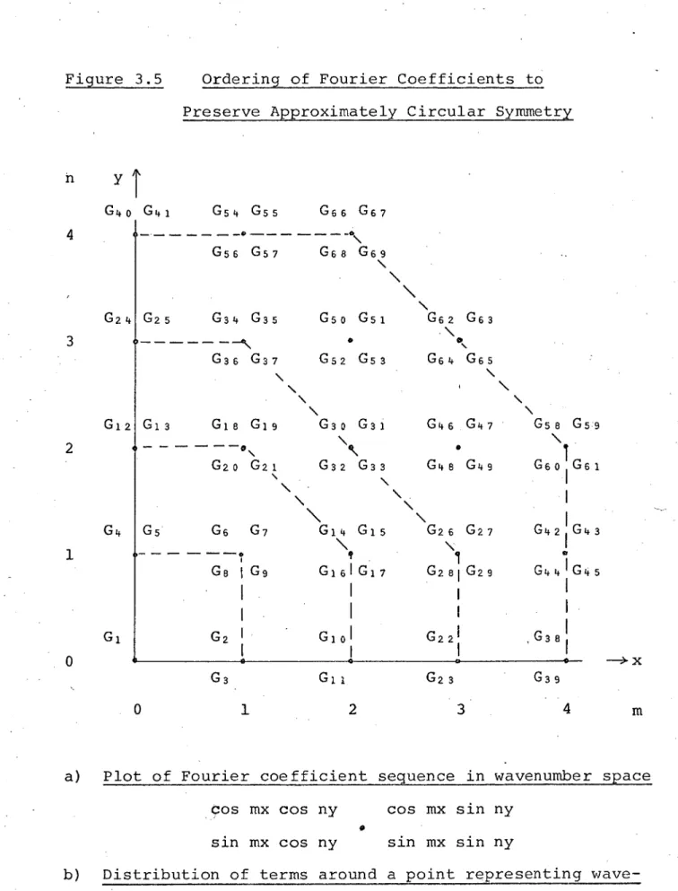
The relationship between, i, the number of the function, and m and n is given in Table 3.2, and in Figure 3.5. It can be seen that radial symmetry has been preserved as far as
possible in order that no undue directional bias be introduced into the data.
The Gram Schmidt orthogonalisation produces a new set of functions, F, which are orthogonal with respect to the data distribution. In this process each function is computed, by ensuring its orthogonality with all the previous functions, at each data point (x k , Yk)
Hence, F i (x k ,y k ) = Gl (ck ,yk ); k= 1, and for successive functions, i = 2, imax
i - 1
y
' F.(x
' ) = G.(x y ) -
I k k 1 k k 'X i . 1 a ij F. (x k ,y k ); k = 1, N G. (x k ,y k ) F j (xk ,yk )
k = 1
(Fj (xkl yk )) 2 k = 1
where a.. = 13
Table 3.2
Wave number
0 Gi = 1
Function Set Chosen for Gram Schmidt Orthogonalisation Process
G. ( x, y )
—a
1 G2 = cos x G3 = sin x
G6 = cos x cos y G7 = cos x sin y
•
2 G 1 0 = cos 2x Gil = sin 2x
. G14 = cos 2x cos y GI5 = cos 2x sin y
GI8 = cos x cos 2y G19 = cos x sin 2y
Gy = cos y
G8 = sin x cos y
G12 = cos 2y
GI6 = sin 2x cos y
G20 = sin x cos 2y
G5 = sin y
Gg = sin x sin y
GI3 = sin 2y
G17= sin 2x sin y
G21 = S111 x sin 2y
3 G22 = cos 3x G 23 = sin 3x G24 = cos 3y G25 = sin 3y
G26 = cos 3x cos y G27 = cos 3x sin y G28 = sin 3x cos y G29 = sin 3x sin y
G30 = cos 2x cos 2y G3I = cos 2x sin 2y G32 = sin 2x cos 2y G33 = sin 2x sin 2y
G34 = cos x cos 3y G35 = cos x sin 3y G36 = sin x cos 3y G37 = sin x sin 3y
4 G38 = COS 4x G39 = sin 4x
G42 = cos 4x cos y 'G4 3 = cos 4x sin y
G46 = cos 3x cos 2y G47 = cos 3x sin 2y
G50 = cos 2x cos 3y G5I = cos 2x sin 3y
Gsy = cos x cos 4y G55 = cos x sin 4y
G58 = cos 4x cos 2y G59 = cos 4x sin 2y
G62 = cos 3x cos 3y G63 = cos 3x sin 3y
G66 = cos 2x cos 4y G67 = cos 2x sin 4y
G40 = cos 4y
G44 = sin 4x cos y
G48 = sin 3x cos 2y
G5 = sin 2x cos 3y
G56 = sin x cos 4y
G60 = sin 4x cos 2y
G64 = sin 3x cos 3y
G68 = sin 2x cos 4y
G41 = sin 4y
G45 = sin 4x sin y
G49 = sin 3x sin 2y
G53 = sin 2x sin 3y
G57 '= sin x sin 4y
G61 = sin 4x sin 2y
G65 = sin 3x sin 3y
\ ,
1 G9 G181G17
1 1
1 1
G9 G281G29 r! Q44 In ,J45 1 1
1 1 r 1
G2 G10 1 G22I k738,
Figure 3.5 Ordering of Fourier Coefficients to
Preserve Approximately Circular Symmetry
Y
G40 G41 G54 G55
G56 G57
G66 G67
G6 8 G69
4
G24 G25
3
GI2 G13
2
G4
\
G34 G35 G50 G51 G62 G63
\
— --61/4. • • ■
G36 G37 G52 G53 G64 G65
\ \
\ \
\ \
\ \
G18 G19 G30 G31 G46 G47 G58 G59
\- \
\ N ,
I,
- -, •
G20 G21 G32 G33 G48 G49 u60,u61
\ \ I
\ 1
\ \
\ \ , 1 0
G6 G7 G14 G15 G26 G27 u42 u,43
\
1
G1
G3 G11 G23 G39
1 2 3 4
a) Plot of Fourier coefficient sequence in wavenumber space
cos mx cos fly
sin mx cos ny
cos mx sin ny
sin mx sin fly
b) Distribution of terms around a point representing
3.07
C. = 1 k' k F. (x y ). k k k C (x ,y ) k= 1
i = 1, kmax
(F. (x y )) 2 1 k' k k = 1
The coefficients may be transformed in terms of the
original non-orthogonal function set. This is carried out by the following transformation; for i = 1, kmax;
b.. = 1 11
i - 1
b.. = - I a. b . j = 1, 2, (i - 1)
13 in n3
n = j
the new coefficient set being obtained by
kmax
d.
E
c.b..1 3 31
j = i
The stepwise approximation to the data, Trii (xk ,y k ), of the first m terms of the orthogonal function set is computed from the following relationship
C i F i (xk ,yk ) k = 1, i = 1
3.08
Varm = ((xk ,y k )) 2 - c i 2 (Fi(x k ,y k )) 2 k = 1 k = 1 k = 1
N - m
3.1.4 Orthoganility
Orthogonalisation procedures are often limited in their effectiveness due to accumulated errors in the computations
(e.g. Jones and Gallett, 1962); it is wise therefore to test the orthogonality of the function set before proceeding with the analysis.
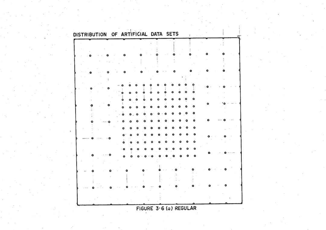
Two artificial data sets were produced to test the effectiveness of the orthogonalisation process. The first, was on a regular basis, the central region having a smaller sampling interval. The second, was similarly produced except the coordinates were chosen from consecutive pairs of a
random number requence. The distributions, referred to as REGULAR and RANDOM, were chosen to simulate the bias in sampling in the real data. The values given to the data
points were calculated from a double Fourier series synthesis, the amplitudes being unity up to a given frequency and zero above. Figure 3.6 shows the distributions of the two
artificial sets of data.
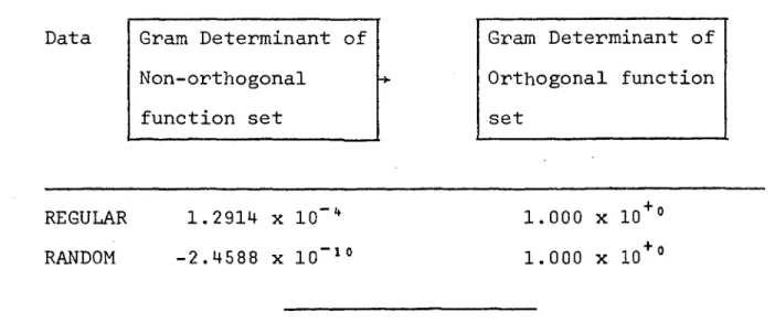
Two different approaches have been used to test for orthoganility. The first method is to test for the
REPEATED CRT HOGONALISA TION TEST
GRAM-SCHMIDT OR THOGONALISA TION FIRST REORTHOGONALISATION SECOND REORTHOGONALISA TION NON-ORTHOGONAL
FUNCTIONS
ORTHOGONAL FUNCTIONS
C 1
OR TN 03 ON AL FUNCTIONS
C2
PERCENTAGE CHANGE
( 02-C 1) /0 1
ORT HOG DNA L FUNCTIONS
C3
PERCENTAGE CHANGE
1C3-32 l/ 02
1 1.000 .2008 12 0+01 .20 0812 0+01 .0000 .200 912 0+0 1 .0300 2 1.000 .1408 60 2+01 .14 0860 2+01 .0000 .140 860 2+0 1 .0 00 0 3 1.000 .14 64 59 0+01 .1404590+31 .5387-06 .146 4593+0 1 .0 CC 0 4 1.000 .11 67 01 7+01 .11 67 01 7+01 -.12 77-0 5 .115 701 7+0 1 -.1915-05 5 1.000 .14 09 05 4+01 .1403364+01 .2544-05 .140 236 4+0 1 .3 00 0
6 1.000 .7436 75 1-CC . 74 36 76 1-00 -.3006-05 .7 436761-C 0 .1 CO 2-05 7 1.003 .94 13 30 0-00 .94 1330 0-0C .5145-0 5 .941 330 0+0 1 .0 00 0 9 1.000 .79 34 19 5-00 . 79 84 195-00 -.46 65-0 6 .7 98419 5-0 0 - .4666-06 9 1 .0 00 .29 95 99 3-00 .92 93 998-00 .74 51 -0 0 .993 539 8-0 0 .3 03 0 10 . .000 -.1928 96 4-07 -. 50 36 74 0-37 .6170+02 - .4 7931 84-0 7 • -.5 08 1+01
11 .030 -.11 2346 0-07 -.6735442-08 -.66 30+C 2 - .9 74 276 8-0 8 .3056+32 12 .000 .3296917-07 .28 83 32 5-C7 -.14 15+0 2 .2 71455 6-3 7 -.6401+01 13 .000 .1041 32 0-06 .9387 95 9-07 -.1092+02 .964 9294-0 7 .2708+01 14 .000 .1C 79 38 0-06 .. 7541 36 1-.37- -.43 13+0 2 .786 303 3-0 7 .4 39 1+01 15 .000 -.8369010-07 -.8337 93 1-07 -.6369+31 - .867 539 1-0 7 .3895+01
15 .000 -.20 76 87 6-06 -. 213653 0-06 .14 08+0 1 -.2 06 2578-0 6 -.2131+01 17 .000 -.26 23 77 1-06 -.20 02 20 3-06 .9594+01 -.2912724-36 .353 3-00 18 .000 -.85 5239 1-07 . -.52 87 294-07 -.61 75+0 2 -.5460671-07 .317 5+01 19 .000 -.23 66 30 5- 06 -.2219471-CS -.3912.01 .- .230 514 7-0 6 .3717+01 20 .030 .77 74 534-07 .55 5747 4-07 -.39 39+0 2 .5 40 637 7-0 7 .2800+31
21 .000 -.43 18 75 3-03 -.61 3187 1-07 .9222+02 -.6605771-07 .6 26 6+01 22 .030 -.9556118-07 -.6435431-27 -.13 68+0 2 -.9136953-37 .3495+01 23 .000 .8127 60 4-07 .8333077-07 .2466 +0 1 .303335 3-0 7 -.2962+01 24 .000 -.7534151-07 -.7142106-07 -.54 89+0 1 - .7 06 214 3-0 7 -.1132+01 25 .02.0 .13 23 33 9-06 .12 1359 2-06 -.5596+01 .1 26 007 6-0 6 .3 29 2+01
..)6 .000 -.1925594-08 -.1502 04 1-07 .8715+0 2 -.1104064-07 -.3505+02 27 .000 -.8780599-37 -. 7532 37 7-87 -.1657+32 -.6779139-07 -.1 11 1+02
23 .000 -.2033569-07 -.47 0241 7-07 .56 82+0 2 - .4 28 147 4-0 7 .5E0 2+01
29 .000 -.6513 77 1-08 .18 80 11 1-07 .1346+0 3 .1 79 388 5-0 7 -.5394+01 30 .000 .1927 78 2-08 -.1517939-03 .1370 +0 4 -.9411222-08 .9839+02
31 ' .000 .3011 13 7-07 -.2512730-39 .1205+05 .1 38 537 9-0 8 .1182+03 32 . .000 -.17 76 68 3-06 -.12 3364 6-05 -.43 51+0 2 - .1 37 005 5-0 6 .9535+01 33 .333 -.3670935-06 -.3623 33 1-06 -.1173+01 -.3614137-06 -.3925-00 34 .000 .51 73 53 3-07 .10 10 23 3-06 .19 09+0 2 .1 05 606 8 -0 6 .4340+01 35 .000 -.21 87 56 3-07 .1340832-07 .3086 +C 3 .7 79 132 1-0 8 -.3462+02
DISTRIBUTION OF ARTIFICIAL DATA SETS