Measures of precision for dissimilarity based multivariate analysis of ecological communities

L E T T E R

Measures of precision for dissimilarity-based multivariate

analysis of ecological communities

Marti J. Anderson,1_{* and}

Julia Santana-Garcon2

Abstract

Ecological studies require key decisions regarding the appropriate size and number of sampling units. No methods currently exist to measure precision for multivariate assemblage data when dis-similarity-based analyses are intended to follow. Here, we propose a pseudomultivariate dissimi-larity-based standard error (MultSE) as a useful quantity for assessing sample-size adequacy in studies of ecological communities. Based on sums of squared dissimilarities,MultSEmeasures var-iability in the position of the centroid in the space of a chosen dissimilarity measure under repeated sampling for a given sample size. We describe a novel double resampling method to quantify uncertainty in MultSE values with increasing sample size. For more complex designs, values ofMultSEcan be calculated from the pseudoresidual mean square of aPERMANOVAmodel, with the double resampling done within appropriate cells in the design. R code functions for implementing these techniques, along with ecological examples, are provided.

Keywords

Assemblage data, community ecology, dissimilarities, multivariate analysis,PERMANOVA, precision, replicates, sampling design, standard error, variability.

Ecology Letters(2015)18: 66–73

INTRODUCTION

Studies of ecological communities require key logistic deci-sions regarding the size and number of individual sampling units that should be used in order to characterise (and ana-lyse) communities of interest. Researchers designing manipula-tive experiments or embarking on mensuramanipula-tive sampling designs (sensu Hurlbert 1984) may well ask the essential ques-tion: How many replicate sampling units are needed to get reasonably precise measures of multivariate variability for purposes of testing relevant null hypotheses regarding commu-nity structure?

To measure the density or relative abundance of a single species (univariate), methods exist to allow researchers to assess (e.g. from a series of replicates obtained in preliminary pilot investigations) the adequacy of any given choice of sam-pling-unit size and/or number (e.g. Andrew & Mapstone 1987; Downing & Downing 1992). In particular, for univariate data one may calculate a value ofprecisionfor the mean of a given sample of n units of a given size. Precision measures the degree of concordance among multiple estimates of a given parameter (such as the mean) for the same population (Cochran & Cox 1957). This is reflected by the variability of an estimate; precision improves as variability decreases. Precision is measurable from the sampling programme and improves with increases in the number and size of sampling units.

An appropriate measure of univariate precision of the mean for quantitative abundance data can be calculated from a given sample as the standard error of the mean; namely,

SE¼s=pffiffiffin, wheres is the sample standard deviation andnis

the number of sampling units. As values ofSE decrease, pre-cision improves. Measures of prepre-cision can be calculated from pilot data, a plot of SE vs. ncan be drawn, and we expect a gradual decrease and apparent levelling-off in the value ofSE

with increasingnin such a plot. One may then consider that a value of n around this apparent asymptote in SE (i.e. where the slope of the curve becomes very small) would be reason-able to use for future investigations of the population mean, as further increases in n would not result in substantially greater increases in precision. A standardised measure of pre-cision of the mean is given by p¼SE=y, where yis the sam-ple mean. This measure is unitless and allows comparisons among different studies. Also, given a set of pilot data, one may calculate a value of n required to achieve a desired level of standardised precision seta priori (such as p=0.2, etc.) as

n¼ ½s=ðpyÞ2, rounded up to the nearest integer (e.g. Andrew & Mapstone 1987).

For multivariate data, especially multi-species count data that are gathered with the intention of characterising ecologi-cal communities, there is no obvious measure of multivariate precision that can be used to assist researchers in decision-making processes regarding adequate sampling. First, what do we mean by ‘the community’? We presume here that the researcher has already defined the community conceptually initially by reference to a particular spatial and temporal inferential domain (e.g. trees on Great Barrier Island, inverte-brates within a given depth-range on the Norwegian continen-tal shelf within a particular pre-defined area specified by latitude and longitude, etc.). This domain is also likely to include specificity caused by logistic constraints in sampling

1

New Zealand Institute for Advanced Study (NZIAS), Massey University, Albany Campus, Private Bag 102 904, Auckland, 0745, New Zealand

2

The UWA Oceans Institute (M470) and School of Plant Biology, The University of Western Australia, Perth, Australia

*Correspondence: E-mail: [email protected]

organisms which further limits inference (e.g. only macroin-vertebrates large enough to be retained on a 0.5 mm sieve, only trees greater than a certain diameter at breast height (dbh), etc.). Although these decisions might be somewhat arbitrary, often based on convenience or historical legacies (hence, the word ‘assemblage’ is preferable to the word ‘community’ for multispecies data sets, see in particular Underwood 1986), we presume the researcher is sampling from the same ‘universe’ with respect to these definitions within a given study (as in Colwellet al.2004), and that what is required to characterise the community, so defined, from a sampling perspective, will follow directly from this. We acknowledge the complexity of this assumption, however, and recognise that there may be a trade-off when choosing the size of the sampling unit between having enough information about the community and considering the sampling unit to be homogeneous with respect to community structure (Carlile

et al.1989; Drayet al.2012).

Multivariate analyses of ecological communities are very often based on measures of dissimilarity, such as Bray–Curtis, Hellinger or Jaccard, that appropriately emphasise changes in the composition of the identities or relative abundances of individual species (Legendre & Gallagher 2001; Clarke et al.

2006; De Cacereset al.2013). Thus, although a more classical Euclidean-based multivariate analogue of the above univariate precision indices might be considered (e.g. such as the deter-minant of a variance-covariance matrix on normalised data, see also Kotz & Lovelace 1998; Pearn & Kotz 2006), these implicitly or explicitly rely on assumptions of multivariate normality, and are unlikely to shed any light on ecologically relevant compositional information.

Non-parametric measures of precision for multivariate data have been developed recently by Siman (2014). These are based on the calculation of multivariate quantiles using half-space depth regions (Rousseeuw & Ruts 1999; Serfling 2002). For a description of half-space depth (Tukey 1975) and its associated properties, see Dutta et al. (2011). Although these ideas might well be applied fruitfully to sample points in a principal coordinate (PCO) space that preserves a chosen dis-similarity measure (e.g. Gower 1966; Legendre & Anderson 1999; McArdle & Anderson 2001), there remain important problems. The regions must be convex, the calculations require a large number of data points, and the computations are so demanding as to make them unfeasible for any more than four or five variables (Siman 2014). However, data sets in community ecology typically are high-dimensional with many species.

One important aspect of community structure is richness – the number of species – which is known simply to increase with sample size (or sample area). A plot of the cumulative number of species with increases in the number of sampling units (a species-accumulation curve, Gotelli & Colwell 2001; Magurran 2003) can be drawn from a set of samples taken from a given area. The point at which this curve begins to level-off can indicate the number of samples beyond which not many new species will be encountered. The usual purpose of such plots, however, is generally to estimate the total num-ber of species in a given (usually large) area (e.g. Uglandet al.

2003; Colwell et al. 2004; Gray et al. 2004), rather than to

infer the number of sampling units required to characterise variation in community structure within that area. Further-more, the size of individual sampling units is usually driven heavily by logistic constraints (e.g. only 1 m2 plots can be examined within a reasonable length of time in the field while diving under SCUBA, etc.).

Our purpose here is to describe some simple approaches to aid in the assessment of appropriate sampling of ecological communities for subsequent analysis using dissimilarity-based multivariate methods, such as PERMANOVA (Anderson 2001a; Anderson et al. 2008), PERMDISP (Anderson 2006; Anderson et al. 2006) or distance-based redundancy analysis (dbRDA, Legendre & Anderson 1999; McArdle & Anderson 2001).

In some cases, lack of information within individual sam-pling units requires a group of samsam-pling units to be pooled together prior to analysis. If the sizes of individual sampling units are too small, then many units may contain no species at all (leading to undefined dissimilarity values) and there also may be many pairs of units that have no (or very few) species in common, yielding dissimilarity values that are uninformative (Clarkeet al.2006). Some simple methods designed to assist in the choice of the number of replicates to pool in such cases are provided in an Appendix (see Supporting Information)

Presuming an appropriate replicate sampling unit (poten-tially comprised of a number of pooled sub-samples) has been defined, we ask: ‘How many replicates are needed to suffi-ciently characterise the community being sampled with rea-sonable precision for subsequent dissimilarity-based multivariate analysis?’ We propose the use of a pseudo multi-variate dissimilarity-based standard error (MultSE)– a direct analogue to the univariate standard error – as a useful quan-tity for assessing sample-size adequacy for ecological studies. Specifically, MultSE provides a measure of variability in the position of the sample centroid in the space of the chosen dis-similarity measure under repeated sampling for a given sample size. This can be calculated easily from a single set of pilot data or on residuals after fitting some more complex sampling design or model. We further propose a double resampling technique (permutation followed by bootstrapping) in order to quantify uncertainty in MultSE values with increasing numbers (or sizes) of sampling units.

METHODS

A multivariate measure ofpseudostandard error

As a direct analogue to the univariate measure of SE of the mean, we consider a multivariate measure ofpseudo standard error (MultSE, first described by Andersonet al.2001), as fol-lows. Let Y be a (n9p) matrix of n sampling units within which the values of each of k= 1,. . ., p variables have been measured. For example, consider counts of each of p species in each of n quadrats that have been placed at random posi-tions within a particular pre-defined study area. Let D be a (n9n) matrix of dissimilarities{dij}among all pairs of

pseudosums of squares in the space of the chosen dissimilarity measure:

SS¼ X ðn1Þ

i¼1 Xn

j¼ðiþ1Þ

d_ij2=n ð1Þ

This is because the quantity in eqn (1) is also equivalent to the sum of squared distances from individual sampling points to their centroid in the space of the chosen dissimilarity measure, a theorem stated in Legendre & Anderson (1999, see Appendix B therein) and Anderson (2001a), proven by Legendre & Fortin (2010, see Appendix 1 therein). Further-more, dividing this by (n 1) yields a quantity that is directly interpretable as a multivariate measure of pseudo variance in the space of the chosen dissimilarity measure:

V¼ 1

ðn1Þ X

ðn1Þ

i¼1 Xn

j¼ðiþ1Þ

d_ij2=n ð2Þ

Indeed, in the case of a single variable and Euclidean distance,

SS is equal to the usual classical univariate sum of squares andV is equal to the usual classical unbiased measure of the sample variance (Anderson 2001a; Legendre & De Caceres 2013). Unbiasedness is only ensured when sampling is representative of the statistical population under study, as is generally achieved by some appropriate form of random sampling.

Note that the word ‘pseudo’ has been used throughout here to distinguish SS in (1) above from the classical multivariate sums-of-squares-and-cross-products (SSCP) matrix and V in (2) above from the classical multivariate sample variance-covariance matrix. The classical matrices will clearly include measures of relationships among all pairs of variables in the multivariate Euclidean space of the original variables (namely, in the off-diagonal positions of these matrices), whereas these

pseudomeasures do not. Note also that, in the case of multi-variate data and Euclidean distance,SS in (1) is equal to the trace of the classical SSCP matrix andV in (2) is equal to the trace of the classical sample variance-covariance matrix.

Finally, based on the above, a multivariate pseudostandard error therefore can be calculated as:

MultSE¼pffiffiffiffiffiffiffiffiffiV=n ð3Þ

We consider that MultSE in (3) is perfectly suitable as a measure of the variability in the position of the sample cen-troid for a given groupin the space of the chosen dissimilarity measure and within a given study. It provides a novel approach to assess adequacy in sample sizes, as it can be based on a dissimilarity measure of choice (see also Pillar 1998). Note, however, that it produces a value which is not standardised in any way–it will be in the units of the resem-blance measure chosen – hence can only be used within the context of a given study, and cannot be compared among studies. Although standardised univariate precision divides the standard error by the sample mean, this is not possible in the present case because the sample mean is clearly a vector here (being multivariate). Thus, although some chosen value of standardised precision for univariate analysis might be sug-gested as a rule of thumb to be applied to studies across a

given field (e.g. p=0.2 or p=0.5, etc.), the value of MultSE

in (3) is dependent on the scale of the dissimilarity measure chosen and (potentially) also on the number of variables, so no such generalisation for its value across multiple studies is apparent. However, as illustrated by the examples below (see Results), MultSE will still nevertheless be quite useful for examining relative precision for different sample sizes within a given study.

The double resampling method and plots ofMultSEvs. sample size

For simplicity of notation in what follows, let s =MultSE. (The use ofsis justified here, assis commonly used to denote a standard deviation, and here we use it to denote the standard deviation of sample centroids for a given sample size in the space of the dissimilarity measure under repeated sampling.) We propose that, given a set of pilot multivariate data having a total of N sampling units, one may draw a random subset (without replacement) of sizen=2, 3, 4,. . .,Nand for each of these random subsets, a value of s can be calculated, which may be denoted in each case bysp_n¼2;sp_n¼3;. . .;sp_n¼N. The super-scriptphere indicates that the value has arisen from a random subset, whereas the subscript indicates the sample size drawn. Repeat this process for a very large number of random draws (say 10 000), then calculate the mean values obtained across all such random subsets of a given sample size as

s_np_¼2;snp¼3;. . .;snp¼N. A plot of snp¼‘ vs. ‘ for‘= 2, 3,. . ., N will

then provide the graphic we require to assess variability (and hence, the degree of precision) with increasing sample size. We propose that these means be calculated using sampling without replacement (i.e. using a permutation method) specifically to ensure that the values obtained will be unbiased.

Next, we propose that a bootstrapping method be used to draw error bars on the plot. It is clear that the number of possible permutations forn=Nis 1 (i.e. this is simply the full set of data) and further that the number of random subsets without replacement that would yield unique values for

sp_n¼ðN1Þ (equivalent to simply leaving out one observation at a time) is also limited to just Npossible values. Hence, we pro-pose obtaining a further random subset as a random draw

with replacement (i.e. a bootstrap sample), of size n=2, 3, 4,. . ., N and for each of these to calculate a value of s, denoted in each case by s_nb_¼2;s_nb_¼3;. . .;s_nb_¼N. The superscript b here indicates, in each case, that the value has arisen from a bootstrap sample. Consider the 0.025 and 0.975 quantiles of the bootstrap distribution for each sample sizen=‘for‘=2, 3,. . .,Nasq_nb_¼‘ð0:025Þ andq_nb_¼‘ð0:975Þ respectively. Unlike the permutation approach, the bootstrap distribution is known to be biased (e.g. Davison & Hinkley 1997). An empirical esti-mate of the bias, for each sample size‘, is given by:

bn¼‘¼ ðsnp¼‘snb¼‘Þ ð4Þ

Hence, estimates of the 0.025 and 0.975 quantiles that attempt to adjust for the bias are provided by

fq_nb_¼‘ð0:025Þ þbn¼‘gandfqnb¼‘ð0:975Þ þbn¼‘g; ð5Þ

bootstrapping approach to obtain appropriate error bars, we shall refer to this overall process generally as a ‘double resam-pling’ method. We note also that clearly other choices of quantiles may easily be calculated here in a similar fashion (e.g. 0.25, 0.75, etc.), if desired.

We provide R code (R Core Team 2014) in the form of a function (‘MSEgroup.d’) which calculates MultSE sepa-rately for each group in a one-way design, with double re-sampling to obtain means and error bars, in each case, for

increasing numbers of replicates (see Supporting

Information). The routine calculates the means using the permutation approach, whereas the lower and upper quantiles are obtained using the bootstrapping approach, including an adjustment for the bias in the bootstrap, as described above.

Calculating MultSE for more complex designs

The idea of using MultSE as a measure of precision can be readily extended for use with more complex sampling designs by noting that the residual mean square provided from a PER-MANOVAanalysis (Anderson 2001a) is itself a measure of mul-tivariate pseudo error variance in the space of the chosen dissimilarity measure. Suppose some number of multivariate sampling units (and not necessarily the same number) is obtained from each of g groups in a one-way ANOVA design, yielding a total of N sampling units. Then, as described in McArdle & Anderson (2001), let D= {dij} be an (N9N)

dissimilarity matrix, let A = {aij} =f0:5dij2g, and let

G¼ ðI_N1110ÞAðI_N1110Þ be Gower’s (1966) centred matrix, where 1 is a column of 1’s of length N and I is a (N9N) identity matrix. Next, let matrixXbe a (N9g) design matrix of full rank that codes for the full PERMANOVA model, including intercept (e.g. in a one-wayANOVA design, g would be equal to the number of groups). Finally, let matrix H be the usual projection matrix for the design, namely H= X[X0X]1X0. Now, the total sum of squares in the space of the dissimilarity measure is given by tr[G], where ‘tr’ denotes the trace of a matrix. This is equivalent to the sum of the total sum of squares for each individual variable (i.e. added up across all variables) if the original dissimilarity mea-sure chosen was the Euclidean distance. A partitioning according to the one-wayPERMANOVAmodel is then given by

tr½G ¼tr½HG þtr½ðIHÞG; ð6Þ

where tr[HG] is the sum of squares explained by the model and tr[(I H)G] is the residual sum of squares. McArdle & Anderson (2001) go on to describe thepseudo F-statistic:

F¼ tr½HG=ðg1Þ

tr½ðIHÞG=ðNgÞ ð7Þ

A test of significance (P-value) is then obtained via an appropriate permutation method (Anderson 2001b; Anderson & ter Braak 2003). The only component of this procedure that is of interest here, however, is purely the residual mean square from the PERMANOVA model, i.e. the denominator of eqn (7). This estimates error (within-group) variability in the space of the dissimilarity measure and is calculated, in the one-way case, as:

V¼ 1

ðNgÞtr½ðIHÞG ð8Þ

After obtainingVfrom eqn (8), one can then apply eqn (2) to calculate precision and perform the double resampling method for increasing numbers of replicates, as described above. Note, however, that the replicates here occur within the structure of a model framework –a specificANOVA design. This means the double resampling method must be applied separately for increasing numbers of samples within each individual cell in the design. For example, in the case of a one-way ANOVA model, the double resampling is done separately within each group.

We provide R code (function ‘MSE.d’) which calculates

MultSE from the residual mean square of a one-way PERMANOVAmodel, including double resampling, for increasing numbers of replicates, as described above, in Supporting Information.

RESULTS

Choosing an appropriate size or number of replicates usingMultSE

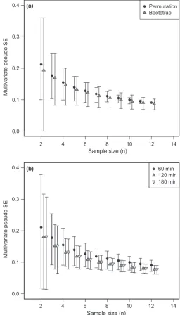
The precision of univariate data has been assessed in order to optimise the sampling effort of baited remote underwater video (BRUV) techniques in estuarine (Gladstone et al.2012) and pelagic environments (Santana-Garcon et al. 2014a,b). The parameters potentially affecting the sampling ability of pelagic stereo-BRUVs include immersion time (the time that cameras are left recording underwater) and the number of replicate deployments.

Data were collected in March 2012 near Tantabiddi Passage in Ningaloo Marine Park (21°530 S, 113°560E), Western Australia. The pelagic stereo-BRUVs used in this study are described in detail elsewhere (Santana-Garcon et al. 2014a,b). The systems were designed to remain in the mid-water at ca. 5 m depth (7.170.54 m, Mean SE), 30 m above the bot-tom and were deployed for an immersion time of up to 3 h. There were 12 replicate deployments (six at each of two sites) obtained during daylight hours. Video images were analysed using the software ‘EventMeasure (Stereo)’ (SeaGIS Pty Ltd, Bacchus Marsh, Victoria, Australia). All fish recorded were quantified and identified to the lowest taxonomic level possi-ble. To avoid repeating counts of individual fish re-entering the field of view, a conservative measure of relative abundance (MaxN) was recorded as the maximum number of individuals of the same species appearing at the same time (Priede et al.

1994). MaxNwas recorded for each of three different immer-sion times: 60, 120 and 180 min.

No previous assessment has been done to optimise multivar-iate precision for dissimilarity-based community analysis of these fish assemblages. We wished to identify: (1) an appropri-ate length of time that cameras should be deployed; and (2) an appropriate number of replicate deployments beyond which no substantial decreases inMultSEwould accrue.

analyses based on square-root transformed abundances and Bray–Curtis dissimilarities. The permutation method alone yields obvious constraints on the error bars for larger sample sizes, whereas the bootstrap method alone yields means that are biased downwards (Fig. 1a). This motivates the use of our double resampling approach, which shows that no appreciable precision is gained by deploying the cameras longer than 120 min, and that a levelling-off inMultSEoccurs for sample sizes around n=7 or 8 (Fig. 1b). The R code used for this

example (‘R code_Ningaloo.txt’) and the original data (‘Ningaloo.csv’) are provided in Supporting Information.

We readily concede that the idea of ‘levelling-off’ must rest in the eyes of the beholder; the approach we suggest is intended to be a heuristic diagnostic tool only, and not a pre-scription. Nevertheless, the analyses of MultSE in this case coincide well with the results obtained for the precision of either of the univariate measures of richness or total abun-dance (Santana-Garcon et al. 2014a). This coincidence might not always occur, however, and will depend on the nature of the data and the characteristics that are emphasised by the chosen dissimilarity measure.

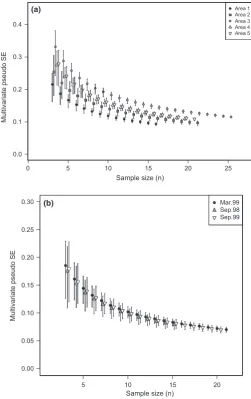
A further example of the proposed method yields additional insight. We consider next an analysis of soft-sediment macro-fauna described by Ellingsen & Gray (2002), who studied beta diversity and its relationship with environmental heterogeneity in benthic marine systems over large spatial scales in the North Sea. Samples of soft-sediment macrobenthic organisms were obtained from 101 sites occurring in five large areas along a transect of 15 degrees of latitude. A total of 809 taxa were recorded overall, and replicate sampling units here con-sisted of abundances pooled across five benthic grabs (sub-samples) obtained at each site. For more details, see Ellingsen & Gray (2002), Ugland et al. (2003) and Anderson et al.

(2006). Of interest here is to identify the number of replicate sampling units required to adequately sample the benthic communities for comparative analysis on the basis of the Jac-card resemblance measure. MultSE was calculated with the double resampling method for increasing numbers of repli-cates separately for each of the five areas. Results show clear heterogeneity in the MultSE values across the five different areas, with the greatest variability occurring in area 3, fol-lowed by areas 4 and 5, then area 2 and finally area 1 (Fig. 2a). This agrees naturally with the differences in multi-variate dispersions found previously (using PERMDISP; Ander-son 2006) using the full set of data (AnderAnder-son et al. 2006, 2008). What is added to our understanding here by consider-ing values of MultSE with increasing sample size (including the double resampling method) is that these differences in dis-persion are already apparent once sample sizes within each area reach about n=10 to 12 sampling units. Knowledge of what level of sampling may be required to identify significant heterogeneity can be quite useful. When dealing with large areas, for example, better estimates of overall richness can be obtained by generating species accumulation curves for each of several smaller sub-sampled areas, due to heterogeneity in community structure (turnover) across the larger sampling extent (Ugland et al. 2003, 2005). The R code used for this example (‘R code_Norway.txt’) and the original data (‘Nor-way.csv’ and ‘Areas.csv’) are provided in Supporting Informa-tion.

CalculatingMultSEfrom a dissimilarity-based residual mean square

Consider data on fish assemblages from the Poor Knights Islands in New Zealand, described by Willis & Denny (2000) and Anderson & Willis (2003). Divers counted temperate reef fishes belonging to each of 62 species in each of nine 25 0.3

0.4 _Permutation

Bootstrap

0.1 0.2

Multivariate pseudo SE

2 4 6 8 10 12 14

0.0

Sample size (n)

0.4

0.3

60 min 120 min 180 min

0.0 0.1 0.2

Multivariate pseudo SE

2 4 6 8 10 12 14

Sample size (n)

(a)

(b)

m9 5 m transects at each site. Data from the transects were pooled at the site level and a number of sites around the Poor Knights Islands were sampled at each of three different times: September 1998 (15 sites), March 1999 (21 sites) and Septem-ber 1999 (20 sites). These span the point in time when the Poor Knights Islands were classified as a no-take marine reserve (October 1998).

Analyses ofMultSEwith the double resampling method vs. increasing sample sizes for each of the three times of sampling (based on log(x+1)-transformed data and Bray–Curtis dis-similarities), was initially done separately for each time and showed no sign of heterogeneity of dispersions, unlike the Norwegian macrofauna (cf. Fig. 2b and Fig. 2a). A pooled estimate ofMultSEcan therefore legitimately be used as a

sin-gle measure of precision, calculated from the residual mean square of a PERMANOVA model (quantity V from eqn (8) above) for the three groups corresponding to the three times of sampling (Fig. 3). Precision in this case is seen to level off and does not improve substantially for these assemblages once the number of sites sampled within each time reaches

around 7 or 8 (Fig. 3). The R code used for this

example (‘R code_PoorKnights.txt’) and the original data (‘PoorKnights.csv’) are provided in Supporting Information.

DISCUSSION

We have provided some quantitative tools for assessing an appropriate number and scale of sampling units for dissimilar-ity-based multivariate analysis of ecological data. We propose here a measure of precision for multivariate data (MultSE) based on inter-point dissimilarities that is a direct analogue of the well-known univariate standard error. More specifically,

MultSE measures the amount of variation in the position of the centroid in the space of the chosen dissimilarity measure under repeated sampling for a given sample size. As such, it is clearly highly relevant for assessing sampling adequacy when the goal is to embark on dissimilarity-based multivariate analyses with specific null hypotheses regarding differences among group centroids in such a space (Anderson & Walsh 2013). A double resampling method allows unbiased measures of variation inMultSEto be obtained.

We recognise the clear limitations of this approach. The measure takes no account of the shape of the multivariate data cloud, only its overall dispersion (size). Future develop-ments should include better characterisation of the actual shape of the data cloud in the dissimilarity space of interest. This might be achieved, for example, through the use of

mul-0.4

Area 1 Area 2 Area 3 Area 4

0.2 0.3

Area 5

0.0 0.1

Multivariate pseudo SE

Multivariate pseudo SE

0 5 10 15 20 25

Sample size (n)

0.30 Mar.99

Sep.98 Sep.99

0.15 0.20 0.25

0.05 0.10

5 10 15 20

0.00

Sample size (n) (a)

(b)

Fig. 2Multivariate pseudo standard error (MultSE) as a function of sample size (a) for each of 5 different areas on the basis of Jaccard dissimilarities for macrofaunal communities from the Norwegian continental shelf and (b) for each of three different times on the basis of Bray–Curtis dissimilarities calculated on log(x+1)-transformed counts of fishes from the Poor Knights Islands, New Zealand. A double resampling scheme was used to generate means for each sample size using 10 000 permutations and error bars as bias-adjusted 2.5 and 97.5 percentiles from 10 000 bootstrap resamples.

0.25 0.30 0.35

0.10 0.15 0.20

5 10 15

0.00 0.05

Sample size (n)

MultSE based on residual mean square

Fig. 3 Multivariate pseudo standard error (MultSE) calculated from the residual mean square of a one-way PERMANOVAmodel as a function of

tivariate kernel density estimation (KDE) in the PCO space of the resemblance measure. This would require, however, enhanced computer power and programming to cope with analyses of high-dimensional data sets like those typically found in ecology. Furthermore, the use of KDE would also concomitantly require large sample sizes to be effective, which could ultimately limit its utility in the present context. Future work should focus also on how such approaches might com-pare with, say, a more classical approach to measure multi-variate precision, such as the determinant of a normalised variance-covariance matrix in the PCO space.

A further limitation of the approach outlined here is its scale dependency. Values of MultSE will necessarily depend on the dissimilarity measure used, so cannot be easily com-pared across studies. More work is needed to assess what lev-els of precision (as measured byMultSE) might be acceptable for different resemblance measures that are bounded and have a common scale, such as Jaccard or Bray–Curtis. Further-more, we consider it is wise, before embarking on dissimilar-ity-based modelling, to examine the distributions of dissimilarities directly to check if large numbers of values approach the limits of what the chosen dissimilarity measure is able to measure. If so, then perhaps the choice of dissimi-larity measure should be revisited. Another possibility is that large numbers of sparse sampling units are present which should be pooled together to provide enough information regarding the community of interest prior to subsequent analysis. We have provided a general tool for assessing the numbers of sub-samples that might be pooled together to define a reasonable ‘replicate’ in this context (see the Data S1).

Finally, although we have described the analysis of preci-sion using the residual mean square from aPERMANOVAmodel only for a one-way case, extensions to higher-way models are clearly very easy to implement using the formulation in eqn (8) for any model specified fully within matrixXand with appropriate associated residual degrees of freedom. In addi-tion, estimates ofpseudocomponents of variation in the space of a dissimilarity measure can be calculated not just for the residual, but also for other individual terms in more complex PERMANOVA models, such as those that arise from hierarchical sampling designs or mixed models (e.g. Andersonet al. 2005; Terlizzi et al. 2007). Empirical measures of variability in the sizes of such components can be estimated using bootstrap-ping approaches (as in Terlizziet al. 2007), thus opening the door to quantifying and assessing the adequacy of sampling at each of a number of spatial and/or temporal scales for mul-tivariate community data – clearly a topic for future study. Some care may be needed in such cases, however, to ensure that the double resampling is performed within appropriate combinations of factor levels, given the particular higher-way design and the particular component(s) of interest.

ACKNOWLEDGEMENTS

MJA was supported by a Royal Society of New Zealand Mars-den Grant MAU1005. Logistic support for acquiring the data analysed here from Western Australia was provided by the Uni-versity of Western Australia and the Department of Fisheries,

Government of Western Australia. We thank K. R. Clarke, P. Legendre and two additional anonymous reviewers for provid-ing constructive critical comments to improve the manuscript.

AUTHORSHIP

The ideas and methods presented in this manuscript were con-ceived by MJA who also wrote the text, JSG provided the motivating data sets from the Abrolhos Islands and Ningaloo Reef and also contributed to early drafts and final revisions.

REFERENCES

Anderson, M.J. (2001a). A new method for non-parametric multivariate analysis of variance.Austral Ecol., 26, 32–46.

Anderson, M.J. (2001b). Permutation tests for univariate or multivariate analysis of variance and regression.Can. J. Fish. Aquat. Sci., 58, 626– 639.

Anderson, M.J. (2006). Distance-based tests for homogeneity of multivariate dispersions.Biometrics, 62, 245_–253.

Anderson, M.J. & ter Braak, C.J.F. (2003). Permutation tests for multi-factorial analysis of variance.J. Stat. Comput. Simul., 73, 85_–113. Anderson, M.J. & Walsh, D.C.I. (2013). What null hypothesis are you

testing? PERMANOVA, ANOSIM and the Mantel test in the face of heterogeneous dispersions.Ecol. Monogr., 83, 557–574.

Anderson, M.J. & Willis, T.J. (2003). Canonical analysis of principal coordinates: a useful method of constrained ordination for ecology.

Ecology, 84, 511–525.

Anderson, M.J., Saunders, J.E. & Creese, R.G. (2001). Ecological monitoring of the Okura Estuary. Report 1: Results of a pilot study. Technical report prepared by Auckland UniServices for Auckland Regional Council, University of Auckland, New Zealand, p. 29. Anderson, M.J., Diebel, C.E., Blom, W.M. & Landers, T.J. (2005).

Consistency and variation in kelp holdfast assemblages: spatial patterns of biodiversity for the major phyla at different taxonomic resolutions.

J. Exp. Mar. Biol. Ecol., 320, 35–56.

Anderson, M.J., Ellingsen, K.E. & McArdle, B.H. (2006). Multivariate dispersion as a measure of beta diversity.Ecol. Lett., 9, 683–693. Anderson, M.J., Gorley, R.N. & Clarke, K.R. (2008).PERMANOVA+

for PRIMER: Guide to Software and Statistical Methods. PRIMER-E, Plymouth, UK.

Andrew, N.L. & Mapstone, B.D. (1987). Sampling and the description of spatial pattern in marine ecology.Oceanogr. Mar. Biol. Annu. Rev., 25, 39–90.

Carlile, D.W., Skalski, J.R., Batker, J.E., Thomas, J.M. & Cullinan, V.I. (1989). Determination of ecological scale.Landscape Ecol., 2, 203–213. Clarke, K.R., Somerfield, P.J. & Chapman, M.G. (2006). On resemblance

measures for ecological studies, including taxonomic dissimilarities and a zero-adjusted Bray-Curtis coefficient for denuded assemblages.

J. Exp. Mar. Biol. Ecol., 330, 55–80.

Cochran, W.G. & Cox, G.M. (1957). Experimental designs, 2nd edn.. John Wiley & Sons, New York.

Colwell, R.K., Mao, C.X. & Chang, J. (2004). Interpolating, extrapolating, and comparing incidence-based species accumulation curves.Ecology, 85, 2717–2727.

Davison, A.C. & Hinkley, D.V. (1997). Bootstrap Methods and Their Application. Cambridge University Press, Cambridge.

De Caceres, M., Legendre, P. & He, F. (2013). Dissimilarity measurements and the size structure of ecological communities.

Methods Ecol. Evol., 4, 1167_–1177.

Downing, J.A. & Downing, W.L. (1992). Spatial aggregation, precision, and power in surveys of freshwater mussel populations. Can. J. Fish. Aquat. Sci., 49, 985–991.

Dutta, S., Ghosh, A.K. & Chauduri, P. (2011). Some intriguing properties of Tukey’s half-space depth.Bernoulli, 17(4), 1420–1434.

Ellingsen, K.E. & Gray, J.S. (2002). Spatial patterns of benthic diversity: is there a latitudinal gradient along the Norwegian continental shelf?

J. Anim. Ecol., 71, 373–389.

Gladstone, W., Lindfield, S., Coleman, M. & Kelaher, B. (2012). Optimisation of baited remote underwater video sampling designs for estuarine fish assemblages.J. Exp. Mar. Biol. Ecol., 429, 28–35. Gotelli, N.J. & Colwell, R.K. (2001). Quantifying biodiversity: procedures

and pitfalls in the measurement and comparison of species richness.

Ecol. Lett., 4, 379–391.

Gower, J.S. (1966). Some distance properties of latent root and vector methods used in multivariate analysis.Biometrika, 53, 325–338. Gray, J.S., Ugland, K.I. & Lambshead, J. (2004). Species accumulation

and species area curves–a comment on Scheiner (2003).Global Ecol. Biogeogr., 13, 473_–476.

Hurlbert, S.H. (1984). Pseudoreplication and the design of ecological field experiments.Ecol. Monogr., 54, 187_–211.

Kotz, S. & Lovelace, C.R. (1998).Process Capability Indices in Theory and Practice. Oxford University Press, New York.

Legendre, P. & Anderson, M.J. (1999). Distance-based redundancy analysis: testing multispecies responses in multifactorial ecological experiments.Ecol. Monogr., 69, 1–24.

Legendre, P. & De Caceres, M. (2013). Beta diversity as the variance of community data: dissimilarity coefficients and partitioning.Ecol. Lett., 16, 951–996.

Legendre, P. & Fortin, M.-J. (2010). Comparison of the Mantel test and alternative approaches for detecting complex multivariate relationships in the spatial analysis of genetic data.Mol. Ecol. Resour., 10, 831–844. Legendre, P. & Gallagher, E.D. (2001). Ecologically meaningful

transformations for ordination of species data.Oecologia, 129, 271–280. Magurran, A.E. (2003). Measuring Biological Diversity. Blackwell

Publishing, Oxford.

McArdle, B.H. & Anderson, M.J. (2001). Fitting multivariate models to community data: a comment on distance-based redundancy analysis.

Ecology, 82, 290_–297.

Pearn, W.L. & Kotz, S. (2006).Encyclopedia and Handbook of Process Capability Indices. World Scientific Publishing, Singapore.

Pillar, V.D.P. (1998). Sampling sufficiency in ecological surveys. Abstr. Bot., 22, 37–48.

Priede, I.G., Bagley, P.M., Smith, A., Creasey, S. & Merrett, N.R. (1994). Scavenging deep demersal fishes of the Porcupine Seabight, Northeast Atlantic - Observations by baited camera, trap and trawl.J. Mar. Biol. Assoc. U. K., 74, 481–498.

R Core Team. (2014). R: A Language and Environment for Statistical Computing. R Foundation for Statistical Computing, Vienna, Austria. ISBN 3-900051-07-0, URL http://www.R-project.org/.

Rousseeuw, P.J. & Ruts, I. (1999). The depth function of a population distribution.Metrika, 49, 213–244.

Santana-Garcon, J., Newman, S.J. & Harvey, E.S. (2014a). Development and validation of a mid-water baited stereo-video technique for investigating pelagic fish assemblages.J. Exp. Mar. Biol. Ecol., 452, 82– 90.

Santana-Garcon, J., Newman, S.J., Langlois, T.J. & Harvey, E.S. (2014b). Effects of a spatial closure on highly mobile fish species: an assessment using pelagic stereo-BRUVs.J. Exp. Mar. Biol. Ecol., 460, 153–161. Serfling, R. (2002). Quantile functions for multivariate analysis:

approaches and applications.Stat. Neerl., 56, 214–232.

Siman, M. (2014). Precision index in the multivariate context.Commun. Stat. Theor. Methods, 43, 377–387.

Terlizzi, A., Anderson, M.J., Fraschetti, S. & Benedetti-Cecchi, L. (2007). Scales of spatial variation in Mediterranean subtidal sessile assemblages at different depths.Mar. Ecol. Prog. Ser., 332, 25_–39.

Tukey, J.W. (1975). Mathematics and the picturing of data. In:

Proceedings of the International Congress of Mathematicians, Vol. 2. (ed. Vancouver, B.C.), Canad. Math. Congress, Montreal, Quebec, pp. 523–531.

Ugland, K.I., Gray, J.S. & Ellingsen, K.E. (2003). The species-accumulation curve and estimation of species richness. J. Anim. Ecol., 72, 888–897.

Ugland, K.I., Gray, J.S. & Lambshead, P.J.D. (2005). Species accumulation curves analysed by a class of null models discovered by Arrhenius.Oikos, 108, 263–274.

Underwood, A.J. (1986). What is a community? InPatterns and Processes in the History of Life. (eds Raup, D.M., Jablonski, D.). Springer-Verlag, Berlin, pp. 351–367.

Willis, T.J. & Denny, C.M. (2000). Effects of Poor Knights Islands Marine Reserve on demersal fish populations. Report to the Department of Conservation, Research Grant No. 2519, Leigh Marine Laboratory, University of Auckland, Auckland, New Zealand.

SUPPORTING INFORMATION

Additional Supporting Information may be downloaded via the online version of this article at Wiley Online Library (www.ecologyletters.com).

Editor, Jonathan Chase

Manuscript received 12 June 2014 First decision made 8 July 2014

MASSEY RESEARCH ONLINE

http://mro.massey.ac.nz/

Massey Documents by Type Journal Articles

Measures of precision for

dissimilarity-based multivariate analysis of

ecological communities.

Anderson, MJ

2015-01