IN SOUTHEAST TASMANIA
by :
Sjafra Dwipa
Submitted in fullfilment of the requirements
for the degree of
Doctor of Philosophy
University of Tasmania
Hobart, Australia
This thesis contains no material which has been accepted for the award of any
other degree or diploma in any University and, to the best of my knowledge
and belief, contains no copy or paraphrase of material previously published
or written by another person, except where due reference is made.
iott
L
Sjafra Dwipa
This research would not have been possible without assistance from many
people. I would like to thank my supervisors Drs. R.J.G. Lewis, W.D. Parkinson
and D.E. Leaman for their encouragement and patience.
Dr. Lewis allowed me to use the "Pancake" computer program which
provided effective analysis of the TEM data. His broad understanding of geophysics
computer programming has been of great assistance. Dr. Parkinson, whose
long-term involvement in magnetovariational and magnetotelluric research is well-known,
shared his wisdom and lent personal materials relating to the topic. Meetings with
him and preparing a paper has greatly influenced my thinking. Dr. Leaman was
always available to share his expert knowledge of Tasmanian geology and to advise
on relevant field methods. The combined expertise of these three geophysicists has
been invaluable and of enormous benefit to me.
Van Jensen, the Geology Department technical officer spent many hours
modifying equipment and resolving technical problems for which I thank him
sincerely. The help and assistance of Mr. P. Cornish and Mr. A. GilIon in arranging
transport for field work and laboratory work are deeply appreciated.
Field work was made much easier with the co-operation of numerous
farmers and land-owners who allowed this stranger from Indonesia to set up
equipment on their properties, sometimes for weeks on end. Some even moved stock
to enable field work to proceed. Others provided transport across their land and all
showed interest in the project. My field-work experience in Australia will be
long-remembered.
Bowden from the Tasmanian office. I was seconded by the Vulcanological Survey of
Indonesia and my thanks go to my directors for releasing me to study in Australia.
I am indebted to my close friends R. Hermanto and M. Roach for constant
discussions throughout this research. S. Sampan, Aung Pwa, Ai Yang and U.
Hartono, fellow researchers have been understanding colleagues and very good
company.
My stay in Tasmania has been enriched by the friendship of my host family,
the Eldridges. They have supported and encouraged me during my research and have
been caring friends to me and my family. Very special thanks to Margaret Eldridge
who assisted with field work and patiently proof-read this thesis.
In the south-east of Tasmania, Jurassic dolerite forms a partial cover over
much of the area. The sedimentary and volcanic rocks in this region are mainly
Permian or younger. The topography is largely dominated by the local structure of the
dolerite.
Utilizing the magnetotelluric and magnetovariational methods, an
investigation was made of the electrical structure along two cross-sections to lower
crust / upper mantle depths. In conjunction with this study the potential field and
transient electromagnetic methods were used. Two-dimensional gravity and magnetic
modellings delineated the geometry and possible structural origin of several rock
sequences associated with a basin structure. The use of the transient electromagnetic
method placed constraints on the thicknesses and resistivities of the surface layer.
As part of the magnetotelluric analysis package, a new rotation angle and
dimensionality calculation method is introduced and tested with different geometrical
structures. The results when compared to other conventional and the Mohr circle
methods show this new method works well and is simpler and faster.
conductivity contrasts between the resistive block in the eastern part of Tasmania and
the conducting ocean floor.
The results from the one and two-dimensional modelling of magnetotelluric,
gravity and magnetic data indicate that the base of the Permo-Triassic cover with its
stockwork of massive dolerite intrusions, is probably never less than 500 metres
below the surface at the northern cross-section and dips south reaching a depth of
about 800 metres on the southern cross-section. The Ordovician limestone, which
may be a possible source of hydrocarbon deposits, has a bulk apparent resistivity
value of 40 Ohm-m inferred from transient electromagnetic modelling. This rock has a
thickness of about 300 metres and its distribution is restricted to the western part of the
study area which is consistent with the results of the two-dimensional gravity and
magnetic modelling. The dipping discontinuity needed in the models to match the
magnetotelluric data, results in a trough-like structure with depth from the surface to
the bottom of about 6 kilometres. This structure is reflected by a broad and large
gravity anomaly together with slightly negative magnetic anomaly and is believed to be
associated with a trough of Cambrian volcanics. This trough has a northwest -
southeast direction and becomes wider and has more conductive flanks to the south.
by: Sjafra Dwipa
Geology Department, University of Tasmania, Australia
Site Written Corrected Comment
Pg. iii line 17 ... induction vector The direction of horizontal field that corre-lates with maximum vertical field first called induction vector and then Parkinson vector. In some resent publications, it called induc-tion arrow.
Pg. 1 line 19 ... have made magnetotelluric ... ... have made magnetotellurics ...
Pg. 2 line 16 ... magnetovariational ... Definition: see page 50, first paragraph Pg. 2 line 17 ... transient electromagnetic Definition: see page 27, second paragraph Pg. 9 line 1 ... cancealed Y-shaped ... ... concealed Y-shaped ...
Pg. 13 line 17 ... lineaments are clearly exposes ... ... lineaments are clearly exposed ... Pg. 13 line 20 This lineament continue ... This lineament continues ...
Pg. 21 line 24 ... ar this part of Figure 11.3 ... ... at this part of Figure 11.5 ...
Pg. 24 line 2 ... parallel to magnetotelluric sites ... ... parallel to magnetotelluric cross-section II Figs. 11.5 and
11.6
Magnetics (nT) Magnetics field (nT) Broken lines are observed data Solid lines are calculated data
Pg. 31 line 9 ... up to 32 channels. ... on up to 32 channels. 32 Channels = 164 milliseconds delay time Pg. 31 line 14 ... about 33 milliseconds. 33 milliseconds = recorded at 21 channels
Pg. 33 line 3 pa, Pot.
Pg. 48 line 15 ... susceptibility value of 0.0 cgs ... ... susceptibility value of 0.005 cgs Pg. 55 lines 3
and 4
Detailed explanation of eqn. (IV.3 and IV.4) can be seen in Parkinson (1983, pp 332-333) as mentioned in the thesis. Pg. 55 line 16 MR = ( RI ( A )z + RI ( B )1 )1/2- MR = [ ( RIA ) L + ( RIB ) 2 ] V-z
Fig. IV.12 ... (redrawn from Dosso et al. 1985) Pg. 69 line 15 ... raverse for the TE mode ... ... traverse for the TE mode ... Pg. 72 line 1 ... period of 60 seconds. ... period of 60 minutes.
Pg. 85 line 6 ... to determine the large value. ... to determine the larger value. Pg. 85 line 15 ... cartesian coordinate system ... ... Cartesian coordinate system ... Pg. 183 line 13 ... on northern cross-section ... ... on cross-section I ...
Pg. 183 line 14 ... on southern cross-section .. ... on cross-section II ...
Pg. 104 line 8 ... described in section V.3.2. ... described in section V.3.2.4. Pg. 136 line 4 ... tentatively be achived ... ... tentatively be achieved ...
Pg. 136 line 9 This is suitable ... ... This is a reasonable first approximation ... Pg. 138 line 25 ... at the surface layer ... ... of the surface layer ...
Pg. 185 line 25 _ .., to to explain ... ... to explain ...
Page
Acknowledgements.
Abstract.
Thesis contents.
List of figures.
viii
list of tables.
xi
Chapter I.
INTRODUCTION.
1
I. 1 .
General.
1
1.2.
Aim of the study.
6
I. 3 .
Regional geological setting.
7
1.4.
Previous'magnetotelluric and magnetovariational
studies.
9
1.4.1.
Magnetotelluric.
9
1.4.2.
Magnetovariational observations.
9
Chapter II.
POTENTIAL FIELD METHODS.
12
11.1.
IntToduction.
12
11.2.
Original data.
12
11.2.1.
Gravity.
12
11.2.2.
Magnetic.
13
11.3.
Overview of gravity and magnetic maps.
13
11.3. 1 .
Gravity.
13
11.3.2.
Magnetic.
15
11.4.
Rock physical properties.
19
11.5.
Two dimensional modelling.
20
11.6.
Interpretation.
21
11.6.1
Cross-section I.
21
11.6.2.
Cross-section II.
24
11.7.
Summary.
26
Chapter III.
TRANSIENT ELECTROMAGNETIC METHOD.
27
111.1.
Introduction.
27
111.2.
Basic theory.
28
111.3.
Data acquisition.
30
111.4.
Data analysis.
31
111.5.
Field results.
35
111.5.1.
Cross-section I.
35
111.5.2.
Cross-section II.
36
111.6.
Discussion.
37
111.6.1.
Cross-section I.
46
111.6.2.
Cross-section IL
48
Chapter N.
MAGNETO VARIATIONAL METHOD.
49
IV. 1.
Introduction.
49
IV.2.
The basic method.
50
Chapter
IV.4.
IV.5.
IV.6.
IV.7.
V.
Data reduction.
Transfer function and induction vector analysis.
Field results.
Discussion.
MAGNETOTELLURIC METHOD.
52
53
56
66
74
V.1.
Introduction.
74
V.2.
Origin and propagation of electromagnetic field.
74
V.3.
The earth's dimensionality.
77
V.3.1.
The one-dimensional earth.
77
V.3.2.
The two-dimensional earth.
79
V.3.2.1.
Impedance tensor.
79
V.3.2.2.
Coherency.
82
V.3.2.3.
Reliability.
82
V.3.2.4.
Principal direction.
83
V.3.2.5.
New rotation angle and dimensionality method. 85
V.3.2.6.
The skew and ellipticity.
89
V.3.2.7.
The resistivity.
90
V.3.2.8.
The tipper.
91
V.3.2.9.
Induction arrow.
93
V.4.
Equipment and survey procedures.
94
V.4.1.
Introduction.
94
V.4.2.
Field equipment used.
96
V.4.2.1.
Equipment design philosophy.
98
V.4.2.2.
Logistics.
98
V.4.3
Survey procedure.
99
V.4.3.1.
The electric field sensor.
99
V.4.3.2.
The magnetic field sensor.
100
V.4.4.
Summary.
103
V.5.
Data analysis.
103
Chapter VI.
MT SOUNDING RESULTS IN SOUTHEAST
TASMANIA.
107
VI. 1.
Introduction.
107
VI.2.
The cross-section I response.
109
VI.3
The cross-section II response.
118
VI.4.
Comparison of rotation angle calculations.
128
VI.4.1.
Discussion.
133
VI.5.
Summary.
134
Chapter VII.
INTERPRETATION OF MT RESULTS IN SOUTH-
EAST TASMANIA.
136
VII. 1.
Introduction.
136
VII.2.
One-dimensional modelling.
136
VII.2.1.
Cross-section I.
137
VII.2.2.
Cross-section II.
148
VII.3.
Two-dimensional modelling.
157
VII.3.1.
Cross-section I.
157
VII.3.2.
Cross-section IL
169
VII.3.3.
Comment and summary of two-dimensional.
modelling.
175
VII.4.
Discussion.
176
VII.4.1.
Sedimentary basin.
176
VII.4.2.
Deeper structure.
180
REFERENCES.
187
APPENDIXES
Gravity and magnetic data.
V. Temperature conection.
LIST OF FIGURES
Figure
Page
1.1
Location map.
3
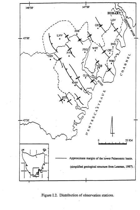
1.2
Distribution of observation stations.
4
1.3
Geology map of the study area.
8
1.4
Induction vectors around Tasmania.
11
II. 1
Residual Bouguer gravity anomaly map of southern Tasmania
14
11.2
Compilation of residual magnetic intensity map.
16
11.3
Compilation of magnetic profiles map at 1000 metres above sea level.
17
11.4
Structural and tectonic interpretation based on gravity and magnetic
data showing major tectonic element.
18
11.5
2D gravity and magnetics model, cross-section I.
23
11.6
2D gravity and magnetics model, cross-section II.
25
111.1
Induction of Eddy currents in a subsurface conductor.
29
111.2
Transient electromagnetic measurement.
29
111.3
Transient electromagnetic Modelling results from Leslie Vale (LSV).
38
111.4
Transient electromagnetic modelling results from Grove (GRV).
39
111.5
Transient electromagnetic modelling results from Judbury (JDB).
40
111.6
Transient electromagnetic modelling results from Lonnavale (LNV).
41
111.7
Transient electromagnetic modelling results from Woodstock (WST).
42
111.8
Transient electromagnetic modelling results from Franklin (FRS).
43
111.9
Transient electromagnetic modelling results from Peppers Rd (PPR).
44
111.10 Transient electromagnetic modelling results from Tahune (THN).
45
IV.1
A sub storm magnetogram, covering 31 hours, showing the principal
features of the storm.
51
IV.2
The open magnetosphere model showing the merging of the field
lines in the magneto-tail.
51
IV.3
Inphase and quadrature induction vectors, period 4 minutes.
57
IV.4
Inphase and quacirature induction vectors, period 8 minutes.
58
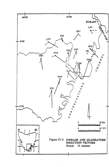
IV.5
Inphase and quadrature induction vectors, period 10 minutes.
59
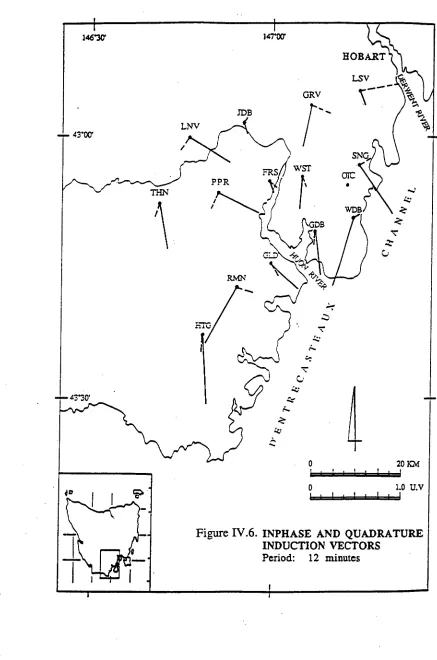
IV.6
Inphase and quadrature induction vectors, period 12 minutes.
60
IV.7
Inphase and quadrature induction vectors, period 16 minutes.
61
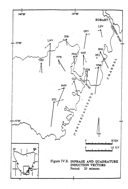
I1.8
Inphase and quadrature induction vectors, period 20 minutes.
62
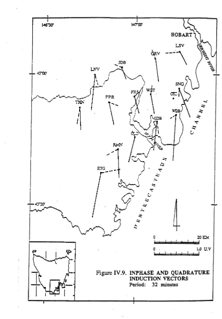
IV.9
Inphase and quadrature induction vectors, period 32 minutes.
63
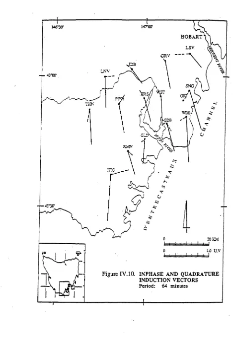
IV.10 Inphase and quadrature induction vectors, period 64 minutes.
64
IV.11
Inphase and quadrature induction vectors,period 128 minutes.
65
IV. 12
Geographical location of Tasmania showing bathymetric contours
around the island.
67
IV.13
Inphase and quadrature vectors for 10 and 60 minutes periods derived
from the analogue model study.
68
IV.14 Observed and corrected induction vectors, period 10 minutes.
71
N.15 Observed and corrected induction vectors, period 60 minutes.
73
V.1
Propagation of an electromagnetic wave (rectangular vectors E and H)
Figure
Page
V.3 X - Y and X' - Y' coordinate system.
86
V.4 Block diagram of EDA FM-1000B Fluxgate magnetometer. 95
V.5 The magnetotelluric equipment.
97
V.6 The magnetic sensor head.
102
VI.1 Principal axes show on a residual Bouguer gravity anomaly map. 108
VI.2 App. resistivity, coherency, skew and phase from Leslie Vale (LSV). 111
VI.3. App. resistivity, coherency, skew and phase from Grove (GRV). 113
VI.4 App. resistivity, coherency, skew and phase from Judbury (JDB). 115
VI.5 App. resistivity, coherency, skew and phase from Lonnavale (LNV). 117
VI.6 App. resistivity, coherency, skew and phase from Oyster Cove (OTC). 119
VI.7 App. resistivity, coherency, skew and phase from Woodstock (WST). 121
VI.8 App. resistivity, coherency, skew and phase from Franklin (FRS). 123
VI.9 App. resistivity, coherency, skew and phase from Peppers Rd. (PPR). 125
VI.10 App. resistivity, coherency, skew and phase from Tahune (THN). 127
VI. 11 Plot of average and delta theta from Judbury (JDB).
129
VI. 12 Plot of average and delta theta from Grove (GRV).
131
VI.13 Plot of average and delta theta from Tahune (THN).
132
VII.1 1D model results from Leslie Vale (LSV).
139
VII.2 1D model results from Grove (GRV).
140
VII.3 1D model results from Judbury (JDB).
141
VII.4 11) model results from Lonnavale (LNV).
142
VII.5 Model of the base of the crust.
145
VII.6 1D TB mode app. resistivity cross-section I, 34 Km depth. 146
VII.6a 1D TE mode app. resistivity cross-section I, 7 Km depth. 147
VII.7 1D model results from Oyster Cove (OTC).
149
VII.8 1D model results from Woodstock (WST).
150
VII.9 11) model results from Franklin (FRS).
151
VII.10 1D model results from Peppers Rd. (PPR).
152
VII. 11 1D model results from Tahune (THN).
153
VII. 12 1D TB mode app. resistivity cross-section II, 34 Km depth. 155
VII.12a 1D TB mode app. resistivity cross-section II, 7 Km depth. 156
VII.13 Model 2D cross-section I.
159
VII.13a Obs. (red) and cal. (green) app. resistivity from LSV and GRV stations
(a) E-polarization, (b) H-polarization.
160
VII. 13b Obs. (red) and cal. (green) app. resistivity from JDB and LNV stations
(a) E-polarization, (b) H-polarization.
161
VII.14 Model 2D cross-section I.
163
VII.14a Obs. (red) and cal. (green) app. resistivity from LSV and GRV stations
(a) E-polarization, (b) H-polarization.
164
VII. 14b Obs. (red) and cal. (green) app. resistivity from JDB) and LNV stations
(a) E-polarization, (b) H-polarization.
165
VII.15 Model 2D cross-section I.
167
VII. 15a Obs. (red) and cal. (green) app. resistivity from LSV and GRV stations
(a) E-polarization, (b) H-polarization.
168
VII. 15b Obs. (red) and cal. (green) app. resistivity from JOB and LNV stations
(a) E-polarization, (b) H-polarization.
169
VII. 16 Model 2D cross-section II
170
VII.16a Obs. (red) and cal. (green) app. resistivity from WST, FRS, and PPR
Figure
Page
VII.17a Obs. (red) and cal. (green) app. resistivity from WST, FRS, and PPR
(a) E-polarization, (b) H-polarization.
174
VII. 18 Plot of 213 MT and gravity and magnetic model along MT cross-
section I
177
VII. 19 Plot of 2D MT and gravity and magnetic model along MT cross-
section II.
179
VII.20 Minimum and maximum bounds on electronic semiconduction
LIST OF TABLES
Table
Page
I.1 List of stations and geographic coordinates.
5
11.1 Density contrast and susceptibility used for rock type within the
study area.
20
INTRODUCTION.
I.1.
General.
The magnetotelluric (MT) method is a frequency-domain electromagnetic
sounding technique used to establish the electrical conductivity of the earth's
sub-surface. This technique utilizes naturally occurring electromagnetic waves as the
energy source. The waves are generated by complex interactions between solar plasma
ejected by the sun and the earth's magnetosphere. These waves penetrate several
hundred kilometres into the earth and induce secondary fields in the earth. The
horizontal components of the resultant electric and magnetic fields are measured at the
surface of the earth. They are related to each other-by a surface impedance that is a
function of the conductivity structure of the earth's substrata. The experimental values
are matched to model curves to obtain an interpretation.
Interpretations of magnetotelluric data are complicated by noise. However,
processing techniques can be used to minimize the scattering effect associated with the
data. Initially, records are obtained as a function of time and they must be processed
to obtain the apparent resistivity as a function of frequency. A Fourier transform must
be used to convert the data from the time domain to the frequency domain.
Tikhonov (1950) realized the potential of using natural electromagnetic fields for
sounding of the earth's crust. One of the milestones in electromagnetic work was the
classic paper of Cagniard (1953) on the theory and interpretation of magnetic and
telluric field relationships.
Cagniard only considered a one-dimensional (1-D) earth consisting of
horizontal, isotropic, planar layers of arbitrary thickness and resistivity. Swift (1967),
Vozoff (1972) and other researchers extended the MT method to two-dimensional (2-
D) geometries. These geometries allow conductivity inhomogeneities to exist in the
horizontal direction as well as the vertical direction. Recent studies by Ting and
Hohmann (1981), Spichalc (1985), Zhdanov and Spichalc (1989 and Cerv and Pek
(1990) have further extended the theory to three-dimensional (3-D) conductivity
distributions. As of present, however, the interpretation of 3-D geometry field data is
in its infancy. In this study one- and two-dimensional earth geometries are presented
and discussed in Chapter V.
145°00 E 14600 E 147 00 E 148°00 E KING ISLE
TASMANIA
FLINDERS
o
100 kmiis
t
:
LOCATION
, .. ••
MAP OF SURVEY AREA
_
4
1114.•. I
.
•
Dev onport ''... .
.... ,
Launceston
.. ... . ... ...
1 ....,.. '
3 1 _ i
i uonvHOBART .
Q
C
Hille: i
i j I
1
40°00 S
1°00 S
2°00 S
[image:19.580.112.531.95.736.2]3°00 S
14700'
...
. . •-■
e... '■
i I . . OR
e /
\
J.DB f I
/ I
/
i 10
/ LNV 1 •
t . . / 1
t• 4. ■ SNG
/
t WST •
t •
arc ;
t FRS
P P• • • i
%TEN •
WDB 1
Gipp
ct
to4310'
:47
0 20 1CM
1 1 1 I I i Iii
Approximate margin of the lower Palaeozoic basin.
(simplified geological structure from Leaman, 1987). i
14610'
4300'
•
HOBART ■
\'
.,'.
(
..
S\IN
1
n/
LSV ) • / (
[image:20.580.66.514.84.757.2]Introduction 4
Table 1.1
List of stations and geographic coordinates
No I Station Code : Latitude ' Longitude Method
1 Leslie Vale LSV i 42°56'40" 147°14'20" MT,MV,TEM
2 Grove GRV , 42°58'00" 147°06'20" MT,MV,TEM
3 Judbury JDB , 42°59'40" 146°55'10" MT,MV,TEM
Lonnavale LNV 43°01'30" 146°49'30" MT,MV,TEM
5 Oyster Cove OTC 43°07'10" 147°00'00" MT
6 Woodstock WST 43°04'30" 147°04'30" MT,MV,TEM
7 Franklin FRS , 43°04'00" 146°19'20" MT,MV,TEM
8 Peppers Road , , 43°07'30" PPR 146°49'40" MT,MV,TEM 9 Tahune THN 43°06'00" 146°43'30" MT,MV,TEM
10 Snug SNG . 43°04'09" 147°12'21" MV
11 Woodbridge WDB 43°09'40" , 147°1 3 ' 1 0" MV
12 Gardners Ba GDB 43°11'22" 147°06'40" MV
13
14
Glendevie
Raminea
GLD
RMN ,.
43°15'00"
43°17'40" ,
146°59'10"
146°53'40"
MV
MV
1.2.
Aim Of The Study.
The primary aim of the study was to develop an understanding of the crustal
structure of the southeast of Tasmania. In particular, the nature of the pre-Permian
geology is very poorly known being obscured by Permo-Triassic and Jurassic dolerite
cover. Only two drill holes in southeasten Tasmania, at Glenorchy and woodbridge,
have reached the
-
pre-Permian basement. Such knowledge may have economic
implications for both mineral and hydrocarbon deposits.
In order to properly fulfil this aim a number of secondary aims emerged:
1. To establish a regional electrical survey in southeast Tasmania by the
transient electromagnetic and magnetotelluric methods.
2.
To develop the technique of rotation of coordinates in magnetotelluric
analysis.
3.
To examine magnetic variations to detect correlations between some fixed
directions of the horizontal magnetic and vertical magnetic fields by the
magnetovariational method. Such correlations are indicative of resistivity
contrasts. Correlations of this type have been reported, for example, by
Pitcher (1972), Hermanto (1985) and Ingham (1988).
4.
To interpret the gravity and magnetic data in terms of major upper crustal
structures.
In brief,, the problem is to obtain information on the crustal structure of
southeast Tasmania: the approach is to use a variety of geophysical techniques and
suitable existing geophysical data and where necessary to develop new methods.
basin. Magnetotelluric interpretations have been found to be the simplest in
sedimentary areas.
Most of the stations were established along the supposed boundary of the
basin (see Figure. 1.2). This is important since reliable determinations of the resistivity
structure of this region have not previously been obtained.
1.3.
Regional Geological Setting.
The region is of high relief which diminishes in height towards the east coast.
The higher elevation of the surrounding ranges is due to the erosionally resistant nature
of the thick dolerite bodies occurring in this area. These dolerites are tholeiites of
mid-Jurassic age (McDougall, 1961; 1962). The regional geology of southeast
Tasmania, which illustrates these features, is shown in Figure 1.3.
Figure 1.3 also indicates that the Jurassic dolerite forms a partial cover over
the upper part of the region. The dolerite has intruded all members of the Parmeener
Supergroup (Permian and Trassic in age) . Dolerite sheets vary in thickness from 200
m at Cygnet to about 400 m on Mt. Wellington (Leaman, 1972; 1975). Sheets drilled
at Woodbridge were about 300 m thick (Farmer and Clarke, 1985).
146°30' 147°00'
43 °00'
43°30' —421
0 20 KM
Terdary sediments
Jurassic dolorite
Triassic units
Permian units
MB Ordovician rocks
[image:24.580.58.515.69.687.2]r.71
Cambrian rocks Precambrian rocksThe main feature of this region is a cancealed Y-shaped trough-like structure
with its major arm extending to the northwest comprising in bulk, Palaeozoic material.
The thickness of the trough fill, interpreted from the magnetic and gravity survey in this
area, is about 5 to 6 km (Leaman, 1990 ; Leaman and Richardson, 1990). The trough
overlaps the margin of Late Precambrian deposition. The Precambrian rocks are also
believed to act as the basement for the whole region.
1.4.
Previous magnetotelluric and magnetovariational studies.
1.4.1.
Magnetotelluric.
The only previous magnetotelluric work in south-east Tasmania was done by
Lewis in 1965. This work, the first in Tasmania, was carried out in the Hobart area and
studied the conductivity of the crust.
Lewis successfully measured magnetic and electric fields at the Hobart airport
and TAU Seismic Vault, University of Tasmania. However, no detailed interpretation
was made due to some of the data being affected by geological and artificial noise.
1.4.2.
Magnetovariational Observations.
The more intensive magnetovariational studies in Tasmania are in the
north-east region. They were started by Lilley (1976), see Figure 1.4, as a part of his study
on geomagnetic variations in south-east Australia. Interesting results from Lilley's
study initiated magnetovariational study by other researchers, including Buyung (1980)
and Hermanto (1985). Buyung concluded that the reversal in direction of induction
vectors on the eastern and western sides of the Tamar River could be due to a zone of
high conductivity below the Tamar River. These results led to Hermanto carrying out a
more detailed induction study in the north-east of Tasmania. This work illustrated the
strong coastal effect on the magnetovariational measurements and identified the
conductive anomaly in the Tamar fracture zone. The extension of this zone in
Figure 1.4. Induction Vectors around Tasmania. Hobart vector is for 40 minutes period, and Smithton, Devonport and Bridport vectors are for 5 - 20 mintues period.
POTENTIAL FIELD METHODS.
11.1.
Introduction.
Potential field methods (gravity and magnetic) have been extensively used in
Tasmania for structural assessment (e.g. Leaman, 1992a). Gravity and magnetic
surveys are often related and combined in this way since the two fields may assess
different facets of the rocks and thus resolve ambiguities inherent in a single approach.
Because of their cost effectiveness and their ability to reveal shallow structures and
constrain the geometry of dolerite bodies, gravity and magnetic methods have long
been used in southeast Tasmania. Using the available data, two-dimensional modelling
was carried out during this study in order to delineate the geometry and sub-surface
geological structure along the transient electromagnetic and magnetotelluric
cross-sections and thus assist interpretation of transient electromagnetic and magnetotelluric
data.
11.2.
Original Data.
H.2.1.
Gravity.
the Tasmania Mines Department. This data is fully terrain corrected to 20 kilometres
and was reduced using a density of 2.67 g/cc.
11.2.2.
Magnetics.
The magnetic interpretation was based on a southern Tasmania residual
magnetic intensity map (Figure 11.2). This aeromagnetic data was surveyed and
compiled by Austirex in 1987 using a Caesium vapour magnetometer with an accuracy
of 0.01 nT at 20 meters sample spacing. The survey was flown at 1 kilometre above
sea level with limited drape flying (150 metres clearance) across the few peaks above
this level (Hartz Mountains and Mt. Wellington). The area was covered by two flight
line directions. East-west lines were flown at 2.5 kilometres spacing with north-south
tie lines at 10 kilometres separation. The survey was carried out originally for Conga
Oil, and permission given by the company made the use of this data possible.
11.3.
Overview of Gravity and Magnetics Maps.
11.3.1.
Gravity.
Figure 11.1 is a residual gravity anomaly map of southern Tasmania. The two
model cross-sections are shown on this map. As can be seen from Figure 11.1 some
major lineaments are clearly exposes i.e. the continuation of the Meydina horst and
Derwent basin. The most conspicuous feature is the lineament which coincides with
the boundary of the Precambrian formations in the south-western of the study area.
This lineament continue very clearly to the southeast.
0
7:00CSZ.3 l'OCCOO.c.
l'OCOSL7
Cl e•••••
••■■•
/■•■■
./.■••
Cl
i
%
••••.\ C
2000g.L7 = I:000;Z;
70w
ITA-1
='! Incau°
3
`
1
.
11
OSZ azIs qsatu ppg
•(6861
‘TI°SPrelPFN
pu trgure D poAoulal
Plog
reuolfai '16 3
-1.1.NYIN . "eTurtusz-j . urotpnos Jo dew Xtruloug ,41z.12 Izn2nos rEnp!sali
-1
.
common in the centre of this area. These anomalies, which reflect the denser
Pre-Permian rocks and Jurassic dolerite, are scattered throughout the entire Huon and
Channel region. This positive anomaly also coincides with the approximate centre and
axis of the Huon mobile zone ('HMZ) (sde figure 11.4).
Superimposed on the residual Bouguer anomaly map are the locations at
which transient electromagnetic and magnetotelluric recording stations were placed.
11.3.2.
Magnetics.
A number of localized ground magnetic and aeromagnetic surveys have been
run in this study area, but much of the work is described in unpublished reports.
Leaman (1973, 1981) provides a list of references for these surveys.
The magnetic field (Figure 11.2) bears little apparent direct relationship to the
gravity field (Figure II.1). As can be seen from the magnetic profile map of Figure
11.3, there are two main magnetic features associated with this study area. The first is
a local magnetic high called the Cygnet anomaly in the middle of the study area. The
second is a regional magnetic high along the southwest edge of the area.
The local magnetic high found in the Cygnet area is related to Cretaceous
syenites and their effect on intruded dolerite. Previous work by Leaman and Naqvi
(1967), and Leaman (1977) has shown that many anomalous spikes occur in this
region and are associated with magnetite at intrusion margins and junctions.
Potential Field Methods 16
• :-.. • ,,st,=; yr.
k :•'''''' --_,=.-.'=---..;..
--4
.-"At -,,,-
..,.... \I I,ttr. • .„. 4,,
-
- • ;iv). . k -,.r. • ' N .\il ■i
.i•A'. ' ---
.. 2 ...
:.,
-B-
.1‘ ,_ ,-11111i' •
..„. .
.ttu.4-3"-1.#;.14i#,_ _ . , --1,---, -1\-- --•
--417V1: - •"_';211i1r.1=§6•-_-:-...;c1r.. n ;
\ :St.) '' AT'O-
4 • • t
•
•i'. -• .. t-l-11
5Z‘7 ., ..*...."-7:
..;,_ :...v„. i)
- ,-. -r":•-..7-_-. ■ ■___--- .. k-V17,7,-_'_': - --417. -..:,.:::. \.... ... - ,t. -,-.-••• e•Y. .,),„
- e..._ . ."----. = ,:.;1:-.: --• ... /?‘ 2 At ,...
'''''. --.1;:';'':'''...:^4■---"' •=•\
kai^k;,'
.
.7i;:n.:, .":" ,...?__ ... ..,--
-i., --- .-.. .
0
.•
;-w-
,,..ri:" ... ... .. _... •, .,... ... - -
. ,....,---. •,. ;2,01
-I
I .`i
-
vi.t
_
-..., %
‘...
"
'
N-
:
• ''..- ••
(
CC i,.._,,...7(.1,
V
. 8
v
1 CO ; : N . .
.
•t•-•;&---':: .
• •iZ‘ --,L-:---.
. ‘, 4, clit . ., , ,..- - •..i...fij . .-.2-,..:: 7S-2...te.
. -;-, -,,,, .,:,:.,-;;: - 4
\ . ' s - - • • • 1 i 141 ,tan - 41
. `".7.': .7:;),:=17-.77:,..". ----..7.X.W , „,..:
,,:i.,1';' , II, L v„...*----2_, ,/,..;:,..:-
■
,.,, r , rr.., ,
...• .- 1
- kv,r • •. ,...„...--_,,11/.
:,, i.. •
..----.--.:.( it 41_1.1"-M, - ' . ., .. .. L. • , - .,/,,,,,,,, ..n;1: ,••■•■1■•••••T, • • 1 • T ‘.,„ t, \.\„. .1 , 1 ..., • , • I ''''' ' ,1;,7 .......- , .. •Iri, .. • ,„1-1.11„.-m e, - % v‘. ir., ore
..• \ ,
4E1 •■ - uk
• 4 r..) \ VJI .. .) i fil
...„..„. • IT, • .3.." ..'- '''''.-s".-:*-
' -• : . .,111! ,
n IA •--`=- 8 ii/A !l • z..-.. ". \‘'.1:--" 1 .1,•". IP ,71,...,:- ?.." , iiedr.s-, ,,. )..) ---"F)1 ,vp
, ,...,....- ,..,, ,....t •-•:.;11; G44 _ ....„....4,-12'''s •tl' .-n,„010,. --- \ .2,...._:::-____ , -Oil ,,,,\ .■-"y",...,,,‘, - .1 -;- - - lis ..',—,...
--- • . ::‘ I .. L.
;3
67,
'-'--
-
-
7
-"...''\
11
'''-
'
--
-
'"
,
•
111-
'\
v.---
----:711.1
"
.
"
.\-
"
..
"‘
Ir•-t
"
.
"'"
/1
. \:,,...0 ..,1
, - . ••
‘`ff n 5200000
...■,1$
";'-',..a.T- - :•240;k3- / IN ,. P• T (-011-4/1 •
" ‘‘) , .24' ..2k4.* • ' ''.''T ...:,. ... I -- ---Zi
l'''. '''..":11.,,-, .% .' ' ..)... ...%. '''A • -• . ....if ■;',,tr• • - ..
' . ' ' ' ' ' -1' DI' Q ut... .17'r - -. '''''' • ' t •
Ilkig
...
.. • -% r-:-'---Z".-
-=}:‘,.-- . - ..-ii. " ■ I , r 7 :• 0 • ---:7:
— !',.■ ...T rIll , „.., P '' - -
.- , .-- _,.i'fj• .1."(L ) ' . •''''.... -- 1 rt,,‘ '.. tot!.
„et
•14.41 1 -••••
: i
fr-T4• -11.0i--'
....,...nn. k ,,-_ r.» • \-) .
" ' ..7"... .• V
i • .
--
. Ri
.1 `.:°1 T'')•.k. „...--- .'1"..' 'N. ' / 7.61••• ' \,) 11Di \ • ••-.'i.
'
\ 4
- -
0),) (.,
.i .---,i
11 --7.• '
.-.."; i -...--,. -....k.›.---,-,2..-
.... .-a'''' ' -
- '. ... • *...'...."'..t.- ri--;;:,----,,t-1 ;*,'".°.?- - .."-ti'!".7N !'. Ag-, ) i ■ 1
• .. • / (1P* L-....• '''.
- 1•■• • • \ .
0
■
-
..1. " 4. 1--, .-trr-\ .,-1T.'c/,-4/
fr.': 'r'k- \''.11‘, ---'■,\ e gi ,,..:- ,-..i.j• , \ --/ • -s A.,;,--.-_,...-, ,,, ,,,,4,„, --.1 p .--., , •/ ;
t.,141 ... ,...,
,..,
,.... • • ,... • e ,...._ . ...., . ••••••••._5170000]
.. _., .
if,SCUTXVIR T RRRRR IP 1111110/111L ZEIT/MT SURTCT
mg 1-\--,;.--i-' \j t
\iv.,
,,,
k -
\ ,)
ing
)
\Sh."----,
/ \--:\,..-L__2---
rOP' \
limmollr
..
CYGN, 1IOW
-
— 1
----
5200000mN
-
' ■
-/g:-.
AS IN§N11111111111. ...,,...rv.,-.1----
c
\ \ /-•,_Q_______I________
...._---
%.-
/
:---
=
c> c
L..
■...10 20
40
50km
500 n
A summary of major tectonic elements deduced from the residual Bouguer
anomaly and aeromagnetic data of Tasmania is given by Leaman and Richardson
(1989) and shown in Figure 11.4. The most striking geological feature shown here are
the western Tasmania mobile zone (WTMZ) in western Tasmania, the Tamar mobile
zone
(rmz)
in eastern Tasmania and the Huon mobile zone (HMZ) in southeast
Tasmania.
11.4.
Rock Physical Properties.
Table 11.1.
Density contrasts and susceptibility used for rock type within the study area
Rock unit
Density contrast with
respect to 2.67 (g/cc)
Susceptibility
(cgs)
Tertiary
-sediment
- 0.60
0.0
Jurassic dolerit
0.23 - 0.25
0.004 - 0.005
Triassics
-0.23 - -0.25
0.0
Permian
-0.12 - -0.15
0.0
Ordovician
-sandstone
0.0 - 0.1
0.0
Cambrian
-volcanic
0.07 - 0.1
0.001
Precambrian
-dolomite
0.0 - 0.1
0.0
- other
0 - 0.007
0.0
11.5.
Two-Dimensional Modelling.
preserved in the continued dataset and must be matched gravimetrically against the
same reference levels.
Appendices 11.1 and 11.2 list the Fourier transform filtered gravity data of
cross-sections I and II. Upward continuation of gravity data is a straightforward
operation, as the surfaces are held in field-free space (Telford et al., 1976) and this
approach has also been tested and used by Leaman (1986a, 1986b).
Areas in which the major part is covered predominantly by igneous Jurassic
dolerite, such as southeast Tasmania, usually have complex magnetic variations.
Basement features are often masked by higher frequency magnetic effects that
originate near the surface. Upward continuation at high level observation reduces these
effects, as well as reducing topographic effects (Leaman D.E., pers. comm.).
The topography profile along cross-sections I and II was obtained from
Tasmania 1:100.000 topographic map sheet index: Tyenna, Derwent, Huon and
D'Entrecasteaux, published by the Lands Department. The surface geological units
which were modelled along these cross-sections were based on the Tasmania
Geological Survey maps 1:250.000 (Leaman, 1972, Farmer, 1985).
11.6.
Interpretation.
11.6.1.
Cross-section I.
depth is placed to provide a broad positive signature. In this trough-like structure, a
magnetic susceptibility of 0.001 cgs and density contrast of 0.1 g/cc has been used.
These are the characteristics of Cambrian volcanic rocks (Leaman, 1987). The depth
of this body from the surface is about 900 metres. Attempts to change this depth
result in higher rms error for both gravity and magnetic calculations. Some spikes on
the observed magnetic field were also found in this section. The two small spikes are
believed to be associated with
-
the Jurassic dolerite bodies that crop out to the west of
Lonnavale.
One of the conspicuous features in this cross-section is a narrow magnetic
high near 30 kilometres (see Figure 11.4). This anomaly has the highest value of +175
nT at 29.5 kilometres and two minimum values of -120 nT at 25.5 kilometres and -185
nT at 33 kilometres respectively (see Appendix 11.1). The major contribution to this
magnetic anomaly is the strongly magnetic Jurassic dolerite, which blankets much of
the study area. The Jurassic dolerite is modelled as intruding the Permian and
Ordovician rocks. The vertical extent of the dolerite is proportional to its width. The
extent of the dolerite shown here has a susceptibility of 0.004 cgs, but in some places,
the dolerite may contain granophyre (Dr. D. Leaman, personal communication, 1992)
which has susceptibility of 0.01 cgs. Consequently the thickness of the dolerite
decreases and intrudes the formation below with pipe-like shape.
(1, u) sap 3u 2ew sp otg al nl W U l v! lual od CROSS-SECTION I 19 17_ 15_ 13_
I I _
9_ 7_ 5 — 3— 1 _ -1_ -3_ -5-- 0 aObs. Gray.
tins error: .09 Gshift: 0
I(X)0_
2000
3(X)0_
E 4(X)0_ .0
4a, 50()0_
60(X)_
8000_
LSV
• Obs. Mag.
rats error: 2.3 Mshift: -50 350 ..300 _250 _200 _150 _ 1(X) _50 _0 -50 _ -1(X) _-I50 _ -2(X) -250 0 _6000 _7000 _8000
= Tertiary (sediment)
= Jurassic (dolerite)
= Triassic (sandstone, mudstone)
7000_ = Permian (mudstone, sandstone, siltstone, limestone)
= Ordovician (limestone) = Cambrian volcanic
= Jubilee-region-style Precambrian (dolomitic)
9000 9000
0 100(X) 200(X) 300(X) 400(X) 500(X) 60000
Distance (m)
Model File: I, I NE1 L.MOD Ohs. ra vi ty:G IZA V IN EW.01IS Ohs. ague( ic:M A GCRS 1.013S Date:01 -04-1993 Time:15:48:45
••=1•11M MO UIMINIM .11.111”.1.1•MMIMIIMMOIMI MIUMMIIIIIM NM MIDIN.M=IMIIM
1((X) 2000
H.6.2.
Cross-section II.
Figure 11.6 shows the observed and calculated gravity and magnetic
cross-section II almost parallel to magnetotelluric sites (THN, PPR, FRS, WST). As can be
seen here the observed gravity profile is slightly different compared to cross-section I.
The gravity profile begins with the negative anomaly of -7 mGal (see Appendix 11.2) at
the western edge of the cross-section and drastically increases at 8 kilometres to form a
relatively large positive anomaly at 30 kilometres with maximum value of 9.5 mGal
increasing toward the east of the traverse. The characteristic mentioned which is
accompanied by a waving pattern of the gravity profile demonstrates that the denser
basement extends irregularly east. The broad and large gravity anomaly together with
slightly negative magnetic anomaly at the middle of the cross-section may be due to a
large Cambrian volcanic body which has a thickness of about 5 kilometres and a base
of from 20 - 33 kilometres.
(1, u) sap a u Sew 10(X) 2000 3(100
E 40(X)__
754, 5(X)0 -A 6(X)0_ 7000 8000_ 9000 300 _250 _200 _150 ..100 50 _0 _ -50 _-150 -200 0 1000 20(X) 30(X) _4(XX) _5000 _6000 _7000 _8000 9000
1 1
1(0(X) 200(X) 30000 400(X) 5((XX) 60000 Distance (m)
Model File:LINE2G.IVIOD Ohs. Gravity:GRA V2NEW.OBS Ohs. Magnetic:MAGVHS2.011S Date:01-04-1993 Time:15:50:41
= Tertiary (sediment) = Jurassic (dolerite)
= Triassic (sandstone, mudstone)
= Permian (mudstone, sandstone, limestone) = Devonian granites (adamalite, granodiorite) = Ordovician (limestone)
= Jubilee-region-style Precambrian (dolomitic)
sp otg aw pi au ivp uaod CROSS-SECTION II 00bs. Gray.
rms error: .06 Cshill: 0
• Obs. Mag. rms error: 3.1
Mshift: -50
a. oat,
"a , 0 • - -a 14 12_ 10_ 8.. 6_ 4 _ 2_ 0_ -2_ -4--6 -8_
THN WST OTC
111.7. Summary.
Some important information can be drawn from the two-dimensional potential
field modelling results: the entire region of these cross-sections is blanketed by
Permo-Triassic rocks intruded by Jurassic dolerite; a major unconformity exists at the
base of the Permo-Triassic (Parmeener Super group) cover;
a
drop in the magneticvalue before the large anomaly is an indication of a deep fault; a trough like structure
with Cambrian Volcanic fill is found at the western part of cross-section I and at the
middle part of cross-section H, suggesting that this structure has a northwest -
TRANSIENT ELECTROMAGNETIC METHOD.
111.1.
Introduction.
Inductive electromagnetic geophysical exploration methods employing a
time-varying artificial primary field as a power source, have been used for many years for
probing the earth's shallow crust. An alternating or a step function current, when
driven into a coil or through a wire grounded at both ends, will produce an oscillating
magnetic field. Any conducting material within the region of the magnetic field will
have generated within it induced currents, which will tend to flow in paths normal to
the direction of the applied magnetic field. These induced, or eddy currents, will in
turn generate a secondary magnetic field which will oppose the primary exciting field
inside the conductor (see Figure I11.1).
Any electromagnetic system operates in the frequency domain involving
continuous transmission at a fixed frequency. Time domain electromagnetic systems,
in which pulses are transmitted and the transient decay of any resultant secondary field
is recorded during the interval between the pulses, have been developed in the last few
decades. The name commonly applied to such systems is Transient Electromagnetic
or TEM for short. The application of the TEM systems in geophysical exploration on
the ground has been reported by many authors.
Cheesman, 1989 and Cheesman et al., 1990). The applications of such tools are
numerous and include assessing off-shore placer mineral deposits, mapping
quarternary geology and, in deep water, studying the physical properties of mid-ocean
ridge hydrothermal regimes and associated massive sulphide deposits.
IH.2.
Basic Theory.
MEASUREMENT' CHANIM.
PRIMARY MAGNETIC FIELD
SECONDARY MAGNETIC FIELD - - -
Figure 111.1. Induction of Eddy currents in a subsurface conductor
(from Geox Sirotem).
PRIMARY FIELD PRIMARY FIELD I
ON OFF
VOLTAGE
!DELAY' TIME ( m.secs. )
•
111.3.
Data Acquisition.
The instrument used for this study was a SIROTEM MK1 transient
electromagnetic system. SIROTEM was developed as a portable transient
electromagnetic system for use in areas of highly conductive overburden, such as
occur widely in Australia (Buselli and O'Neill, 1977), from earlier instruments
invented in the USSR and North America. For a concise history of the development of
transient electromagnetic instruments, see Spies (1980).
The transient electromagnetic systems record data in the time domain, and
SIROTEM can record up to 32 channels of data for delay time from 0.4 msec. to
approximately 160 msec. after the cessation of the transmitter current. SIROTEM
produces, at each survey station, a hard copy of the transient voltages in
nanoVolts/Ampere and can also produce apparent resistivity of the equivalent
half-space at each delay time.
There are a number of different loop configurations possible for transient
electromagnetic measurements, some being better than others for specific geological
situations. The coincident loop configuration was chosen as it has the highest signal
levels of any configuration because the receiver is in the place of strongest
transmission, and therefore best when transmission field is attenuated such as is
caused by conductive overburden (BuseIli et al. 1985)
:
With coincident loops, if
present, the superparamagnetic response causes the ground to appear to be more
conductive and at late times the apparent resistivity values are lower than expected. In
Tasmania problems with a superparamagnetic ground response are minimal.
transmitting loop and the other as receiving loop. The transmitter loop was displaced
4 m from the receiver loop to avoid any possible superparamagnetic response of the
ground. Comprehensive discussion of these superparamagnetic responses may be
found in BuseIli (1982) and Lee (1984).
Eight stations were established in south-east Tasmania for the transient
electromagnetic sounding measurements (see Figure 1.2 and Table 1.1) in order to
place constraints on the thicknesses and resistivities of the surface layers, and to
examine the magnetotelluric data for signs of static shifts (see Appendix VII.2).
Initially, the transient voltage of each station was recorded up to 32 channels.
However, in all eight transient electromagnetic soundings, the last delay-time readings
were corrupted by noise. The instrument includes electronic circuitry used to filter out
noise (power lines, VLF radio transmissions, sferics) but high noise levels will vitiate
interpretation. To this end, selection was made prior to modelling. The noisy data
were not used. The data taken into the model were selected up to about 33
milliseconds.
Time domain measurements enable data to be presented as an apparent
resistivity versus time pseudosection which is similar to the method of presentation of
induced polarization data. Alternatively, as adopted in this study, data can be
presented as a single set of transient events. The name commonly applied to such a
technique is Transient Electromagnetic Sounding or TS. From the single set of
transient events resistivity-thickness can be inferred.
111.4.
Data Analysis.
During this study data analysis was mainly carried out using Olivetti M260
IBM
compatible PC. In order to convert the transient voltage into the apparent
calculation and apparent resistivity transforms include the effect of ramp-function
current waveform. Details of the appropriate calculations for uniform half-space,
layered half-spaces, and apparent resistivities used here are given in Raiche (1984),
Lee and Lewis (1974) and Spies and Raiche (1980). A brief definition of the most
commonly used parameters such as voltage response and apparent resistivity are given
below.
The voltage response was discussed by Lee and Lewis (1974). The method
is based on calculations for a circular loop, and discussed in Spies and Raiche (1980)
and Raiche (1984). Accordingly, the voltage response (V), at time t, of a
homogeneous half-space (conductivity = a, magnetic permeability = p,) for coincident
Tx - Rx loops of area A, excited by a step current I is as follows:
24,FA
V — Iy(x)
Here, y is a function of the dimensionless parameter- x = aith / 4rtt. It is known that
the voltage induced in a square loop differs from that produced in a circular loop by
less than 1% for x = < 6 (Spies and Raiche, 1980).
Making use of the well-known step function response of Lee and Lewis
(1974), equation (III.2), to determine y and from which x can be determined, the
apparent conductivity aa can then be expressed (Spies and Raiche, 1980) as:
aa
=
ztictx1-
1
A
(III.2)
It is found by a scheme in which the value of at is varied to calculate the following
equations and to make S (t) / S
o
(see equation IV.13 and IV.14) approach 1 via an
iterative procedure. The apparent resistivity pa is defined as p
a
= 11th, where al is
the final value of conductivity found at the end of the procedure (Raiche and Spies
(1981) and Raiche (1984). For the coincident loops, the mutual impedance for
half-space may be written:
aj.to 'Co F ( t ) 2
J1(4)d4
Z(t)= t
a
where
F(t) = g( 4
,
1i) - g(4ff)
g(y) = yexp(-y
2
) - frcerfc(y)( 0.5 +y
2
)
=
(t-t
0
)41,
0
ala
2
a = to it
J1 (
4 )
is the Bessel function of the first kind of order one.
4
is the Hankel transform variable.
erfc is the complementary error function.
a is the radius of loop.
From this we have
So =
2 Zo ( t ) iir ago (III.4)
00 F(t) 2
S(t)
=I
a
Ji(4)c14Apparent resistivities are thus calculated from the mutual impedance data via the
iterative procedure which takes a first-order approximation value for the apparent
resistivity and successively improves it until the error between the true value S
o
and
the estimated S, as given by equation (III.4) and (III.5) above is sufficiently small.
The first guess estimate comes from a series inversion of (III.3) and equation 4 of
Spies and Raiche (1980).
The equations outlined in the previous section can be used to generate model
curves of apparent resistivity for varying model layer parameters and loop
configurations. Such model curves can be used to interpret field data in forward
modelling. However, this is a tedious process for any but the simplest models and
PANCAKE modifies a first guess to match the field data in some sense, usually to
minimize the sum of squares of errors. This is the process of inversion or solving the
inverse problem. For the inversions in PANCAKE a linearized least-squares
inversion routine, similar to that described in Jupp and Vozoff (1975) was used to
optimize the model parameters of layer resistivities and thicknesses to match the
measured data.
The inversion of field data to best fit layered models was used for
interpretation. Basically a starting layered model specifies the number of layers above
basement. The starting resistivity values and thicknesses are input into the program as
an initial model together with a set of TEM observations (i.e. voltage versus time).
The program adjusts the model parameters to obtain a least squares fit to the
observation.
Raiche et al. (1985). APRE is one of the most useful statistics in finding the most
parsimonious model consistent with the data. For a detailed calculation see Raiche et
al. (1985). For APRE values less than 15 per-cent the model is considered to be in
keeping with the data.
111.5.
Field Results.
The theory put forward in the previous sections has been used to calculate the
apparent resistivity as a function of time in a 100 m per side of coincident loop for a
number of different layered models. These results were plotted against time ranging
from 0.4 to 33 milliseconds which is the typical range used in this study.
As shown in Figure 1.2, in this study the presentation of the data can be
divided into two cross-sections. Cross-section I includes stations: LSV, GRV, JDB,
LNV while cross-section II is composed of stations: WST, FRS, PPR and THN.
(see Table 1.1 for abbreviations).
The transient electromagnetic results may be merged with the magnetotelluric
results using the method of Sternberg et al. (1988) to examine the magnetotelluric data
for signs of static shifts. This is done in Appendix VH.2. It is appears that static shift
corrections are not important here.
111.5.1.
Cross-section I.
stations the standard errors either mean or RMS are generally less than 9 per cent. In
order to get the best fit for stations LSV, GRV and JOB models were done putting
resistivity decreasing with depth. The values of the standard errors and the APRE
above indicate that a two-layer model is a good representation of the data. Attempts to
fit three-layer and four-layer models to data set produced considerably worse
statistics.
111.5.2
Cross-section II.
As can be seen from Figure 1.2, this cross-section is almost parallel with
cross-section I. The plot of each sounding model is shown from Figures 111.7 to
WO. A similar situation to that at cross-section I is found at this cross-section
survey, as the APRE values are low in most cases. In fact they are lower than
cross-section I as the highest APRE value is 12 per cent which is calculated at station THN.
At stations WST, FRK, and PPR the APRE values are 11, 6.8 and 7.2 per cent
respectively. The standard errors from most stations are quite low but THN station
has a standard error slightly higher than at cross-section I. The highest mean error
calculated is 10.2 per cent at station WST while the highest RMS value of 7.7 per cent
is calculated at T'HN. For other stations the standard error values are less than 8 per
cent. However the mean error is as low as 1.79 per cent and RMS error of 2.73 per
cent is found at station FRS. In this cross-section, to get the best fit for stations WST
and FRS, models were done inserting resistivity increasing with depth, while PPR
and T'HN stations data was modelled with resistivity decreasing with depth. By
judging the values of the APRE and standard errors described above, that fall within
111.6. Discussion.
This study has placed constraints on the thicknesses and apparent resistivities
of the surface layers, which provide valuable aid in interpretation of magnetotelluric
data as discussed in Chapter V.
10.0k 300.0 250.0 .. ! e 0 r200 o -
>. v .4 >150.0 .4 v m .4 m 41 100.0 m a a a 50.0 Initial ..i C v 0.0 -300.0- a m ' o
100 Ohm.m
60 Ohm.m '
Final 0.0 E M V a S o
10.0 20.0 30.0 40.0 Time (msec)
1.0E-3 700.0 0.0
040 10.0 20.0 30.0 40.0 Av.resid error: 9.3% 0.0 Time (msec) Mean error: 5.0%
Rms error: 8. i%