Modified surface tracers
4.1
Introduction
The response of a simple theoretical model, and of the Mk3L ocean model, to the relaxation surface boundary condition was studied in Chapter 3. This was determined to be the most suitable boundary condition for spinning up the ocean model, as it results in a stable climate state. However, it also gives rise to a number of deficiencies in the simulated ocean climate. A reduction in the relaxation timescale leads to some improvements in the properties of the deep ocean, but it remains too cold, too fresh and too buoyant. Furthermore, it leads to increased surface salinity tendency adjustments within the coupled model.
This chapter continues to study modifications to the relaxation boundary con-dition, but investigates the dependence of the simulated ocean climate upon the prescribed sea surface temperatures and salinities. As in Chapter 3, the aim is to obtain high-latitude surface waters which have a realistic peak winter density. In assessing each of the modifications, attention is paid both to the realism of the simulated ocean climate, and to the magnitude of the flux adjustments which are diagnosed for use within the coupled model.
In Section 4.2, the prescribed sea surface temperatures and salinities are modified to reflect the presence of sea ice. By making a crude representation of the effects of brine rejection, it is hypothesised that the peak winter density and salinity of the high-latitude surface waters will be enhanced, and that there will be a corresponding improvement in the properties of the deep ocean.
In Section 4.3, the prescribed sea surface temperatures and salinities are shifted forward in time by one month. It is hypothesised that this will reduce the time lag between the simulated and observed surface tracers which arises, at least in part, from the use of the relaxation boundary condition.
Finally, in Section 4.4, an iterative technique is developed, whereby the response of the ocean model is used to repeatedly modify the prescribed surface tracers. This process converges rapidly towards a solution, producing a set of effective surface tracers. When imposed as the boundary condition on the model, these tracers minimise the errors in the simulated sea surface temperatures and salinities.
104 CHAPTER 4. MODIFIED SURFACE TRACERS
4.2
Sub-ice surface tracers
The sea ice component of the Mk3L coupled model is incorporated into the atmo-sphere model, rather than the ocean model. This has two important consequences:
• the stand-alone ocean model does not incorporate a sea ice model, and can-not therefore directly simulate the effects of brine rejection arising from the formation of sea ice
• within the coupled model, the interface between the atmospheric and oceanic components is located at the ice-ocean interface, andnot the atmosphere-ice interface
The prescribed surface tracers which form the upper boundary condition on the stand-alone ocean model should therefore, in ice-covered regions, reflect the temperature and salinity at the ice-ocean interface, rather than the atmosphere-ice interface. This can be achieved by increasing the prescribed sea surface salinity whenever sea ice is present, to simulate the effects of brine rejection, and by setting the prescribed sea surface temperature equal to the freezing point of seawater.
An attempt was made to modify the prescribed sea surface temperatures and salinities accordingly. The approach employed here can be regarded as a highly simplified version of that of Duffy and Caldeira (1997). They use a simple sea ice model to explicitly calculate the rate of brine rejection, with the salt released during sea ice formation being uniformly mixed throughout the upper 160 m of the water column. Such an approach represents a modification to the model physics, and was not therefore considered to be appropriate here. Instead, observed sea ice concentrations are used to modify the prescribed sea surface temperatures and salinities to reflect the presence of sea ice.
4.2.1 Sea ice concentrations
Climatological monthly-mean sea ice concentrations for the period 1982–2003 were derived from the NOAA Optimum Interpolation v2 analysis (Reynolds et al., 2002). This dataset incorporates not only in situ observations from ships and buoys, but also satellite observations. Analysed values for the sea surface temperature and sea ice concentration are provided on a 1◦×1◦ latitude-longitude grid.
4.2.2 Sea surface temperatures
Beneath sea ice, the water temperature was taken as being equal toTice = -1.85◦C, being the value used by Mk3L for the freezing point of seawater. The World Ocean Atlas 1998 sea surface temperatureTobs was therefore replaced with a modified value given by
T′ obs =
(
(1−f)Tobs+f Tice f ≥0.15
Tobs otherwise
(4.1)
hence the World Ocean Atlas 1998 data was only replaced where the concentration was greater than or equal to this threshold.
4.2.3 Sea surface salinities
Modifying the sea surface salinities was less straightforward than modifying the sea surface temperatures, as there was no single value which could be taken as representing the salinity beneath sea ice. Instead, a more suitable approach was to apply an increment to the sea surface salinity in the presence of sea ice, representing the effects of brine rejection.
Estimates of the contribution of brine rejection to the salinity of Antarctic Bot-tom Water range from ∼0.15–0.2 psu (Toggweiler and Samuels, 1995) to ∼0.9 psu (Broecker, 1986). Given the uncertainty in these estimates, and the fact that they do not provide a value for the salinity enhancement at the ice-ocean interface, it was sought to develop an approach whereby the magnitude of the salinity increment could be estimated. Let the salinity of the ocean beSoce (psu), and let ice of thick-nessH (m) and mean salinitySice(psu) form. The equivalent depth of salt rejected
Hsalt (m) is then given by
Hsalt =
So
ce−Sice 1000
H (4.2)
If this salt is distributed uniformly throughout a mixed layer of depth dz (m), the increase in the sea surface salinity dS (psu) is given by
dS = 1000
Hs
alt
dz
(4.3)
= (Soce −Sice)H
dz (4.4)
Soce can be taken as being ∼35 psu, and Mk3L uses a value for Sice of 10 psu. Thus, given values for H and dz,dS can be estimated using Equation 4.4.
An indicative value of H for each hemisphere can be obtained by dividing the magnitude of the annual cycle in sea ice volume by the mean sea ice extent; this will give an average value for the depth of ice which forms each year. While there do not appear to be any observational estimates of the magnitude of the annual cycle in sea ice volume (Heil, pers. comm.; Massom, pers. comm.), the values simulated by the Mk3L atmosphere model for each of the Northern and Southern Hemispheres is
∼10×1012
m3
(Section 2.4.4). These magnitudes are consistent with those simulated by the CSIRO Mk2 and Mk3 climate system models (Gordon and O’Farrell, 1997; Gordon et al., 2002), and the NCAR climate system model (Boville and Gent, 1998). The Hadley Centre coupled model simulates annual cycles of magnitude
∼25×1012
m3
and∼20×1012
m3
in the Northern and Southern Hemispheres respec-tively, but suffers from excessive winter ice cover (Gordon et al., 2000).
The annual-mean sea ice extent according to the NOAA OI v2 analysis for the period 1982–2003, neglecting monthly-mean ice concentrations less than 15% and weighting the extent by the ice concentration, is 9.4×10¹²
m2
106 CHAPTER 4. MODIFIED SURFACE TRACERS
World Ocean Modified surface tracers Atlas 1998 0.25 psu 0.5 psu 1 psu
Ross Sea 28.06 28.21 28.37 28.71 Weddell Sea 27.98 28.16 28.35 28.74 Nordic Seas 27.96 27.97 28.00 28.06
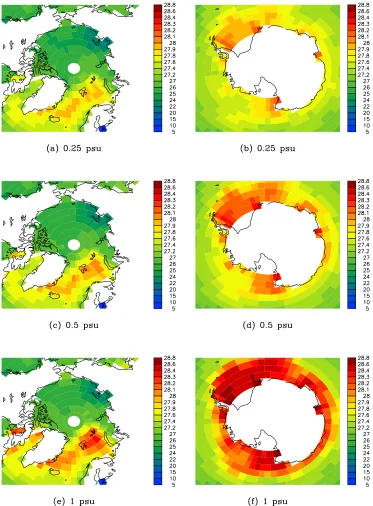
Table 4.1: The peak surface σθ (kgm−3) in regions of deep water formation, for the World Ocean Atlas 1998 data and the modified surface tracers, for salinity increments of 0.25, 0.5 and 1 psu. The data has been area-averaged onto the Mk3L ocean model grid.
Hemisphere, and 10.0×10¹²
m2
for the Southern Hemisphere. Thus it is estimated thatH is equal to ∼1 m for both hemispheres.
A typical value for the mixed-layer depth is∼50 m (e.g.Washington and Parkin-son, 1986). Substituting H = 1 m and dz = 50 m into Equation 4.4, a value is obtained for the salinity increment ofdS = 0.5 psu. However, given the uncertainty regarding a suitable value for dS, three sets of modified sea surface salinities were produced, using increments of 0.25, 0.5 and 1 psu. The World Ocean Atlas 1998 sea surface salinitySobs was therefore replaced with a modified value given by
S′ obs =
(
Sobs+f dS f ≥0.15
Sobs otherwise
(4.5)
4.2.4 Densities of high-latitude surface waters
Figure 4.1 shows the peak high-latitude surface water densities which are implied by the modified sea surface temperatures and salinities; values for the World Ocean Atlas 1998 data are shown in Figure 3.1. The peak densities in the three key regions of deep water formation are also shown in Table 4.1.
The modifications to the sea surface temperatures and salinities lead to signifi-cant increases in the implied peak surface water densities in the Ross and Weddell Seas, with increases of up to 0.65 and 0.76 kgm−3
respectively. However, the peak density in the Nordic Seas is almost unaffected; there is little sea ice cover in this region, and hence the modifications to the sea surface temperatures and salinities are small. Although there are large increases in the implied peak surface densities in the Barents Sea, to the north of Russia, this is not a region of deep water formation.
4.2.5 The response of the Mk3L ocean model
108 CHAPTER 4. MODIFIED SURFACE TRACERS
rates of change in global-mean potential temperature and salinity, on each model level, were less than 0.005◦C/century and 0.001 psu/century respectively). As with
run O-DEF, the durations of the asynchronous and synchronous stages were 4,000 and 500 years respectively.
Water properties
The vertical profiles of potential temperature, salinity and potential density are shown in Figure 4.2. The modifications to the sea surface temperatures and salinities lead to large increases in the salinity and density of the deep ocean, with run O-0.5psu having the most realistic deep ocean salinities, and run O-0.25psu having the most realistic deep ocean densities. However, the modifications also increase the cold bias of the deep ocean, accounting for that fact that the deep ocean of run O-0.25psu has the most realistic densities, even though it is too fresh.
The zonal-mean potential temperature, salinity and potential density are shown in Figures 4.3, 4.4 and 4.5 respectively, as anomalies relative to the World Ocean Atlas 1998; values for run O-DEF are shown in Figures 2.14c, 2.15c and 2.16c. The increased cold bias of the deep ocean is apparent, as is the realistic nature of the deep ocean salinities in run O-0.5psu, and the realistic nature of the deep ocean densities in run O-0.25psu.
The response of the deep Arctic Ocean differs from that of the remainder of the world ocean, however. While it is significantly too warm in run O-DEF, it cools as the salinity increment is increased, and has realistic temperatures in run O-1psu. Likewise, the deep Arctic Ocean was too fresh and too buoyant in run O-DEF, but has realistic salinities and densities in run O-1psu. This suggests, as has been indicated in other studies, that there is a “fair weather” bias in the observed sea surface temperatures and salinities over the Arctic Ocean (Section 3.4.2). Only when they are modified to reflect the presence of sea ice do they become consistent with the observed temperatures and salinities at depth.
Circulation
The rates of North Atlantic Deep Water (NADW) and Antarctic Bottom Water (AABW) formation are shown in Table 4.2. As the salinity increment is increased, the peak densities of the surface waters in the Ross and Weddell Seas increase, and the production of AABW intensifies. However, the resulting increase in the density of the deep ocean, and hence in the stratification of the water column, causes the production of NADW to diminish. Given that the rate of NADW formation in run O-DEF is too weak (Section 2.5.2), this represents a decrease in the realism of the simulated ocean climate.
The increased dominance of AABW formation over NADW formation provides an explanation for the increased cold bias of the deep ocean.
Surface fluxes
110 CHAPTER 4. MODIFIED SURFACE TRACERS
Figure 4.3: The zonal-mean potential temperature (◦C) for the world ocean
112 CHAPTER 4. MODIFIED SURFACE TRACERS
Run Rate of formation (Sv) NADW AABW
O-DEF 13.6 9.5
O-0.25psu 13.0 11.2
O-0.5psu 12.3 11.8
O-1psu 11.8 12.6
Table 4.2: The rates of deep water formation (Sv) for Mk3L ocean model runs O-DEF, O-0.25psu, O-0.5psu and O-1psu (averages for the final 100 years of each run): North Atlantic Deep Water (NADW), and Antarctic Bottom Water (AABW).
which employ an ocean model incorporating Gent-McWilliams eddy diffusion (e.g. Bi, 2002), and contrary to studies which do not (e.g. Weaver and Hughes, 1996), the impact upon the surface fluxes is negligible.
4.2.6 Summary
The prescribed sea surface temperatures and salinities have been modified at high latitudes, in an attempt to reflect the presence of sea ice. Some aspects of the simulated ocean climate are improved, but others are diminished. While it is possible to obtain realistic deep ocean salinities and densities, an increase in the rate of Antarctic Bottom Water formation, combined with a decrease in the rate of North Atlantic Deep Water formation, increases the cold bias of the deep ocean.
This experiment was not, therefore, considered to be a success. However, it has been shown that, by correcting for an apparent “fair weather” bias in the observed sea surface temperatures and salinities in the Arctic, it is possible to improve the properties of the simulated deep Arctic Ocean.
4.3
Phase-shifted surface tracers
4.3.1 Introduction
The flux adjustments employed within the coupled model are diagnosed from the mismatch between the surface fluxes simulated by the stand-alone atmosphere and ocean models (Section 2.6). This methodology assumes that the climates of the stand-alone atmosphere and ocean models are the best that can be obtained, given the spatial resolutions, physical parameterisations and boundary conditions em-ployed (Weaver and Hughes, 1996).
114 CHAPTER 4. MODIFIED SURFACE TRACERS
model is to maintain the ocean in its phase-lagged state. The flux adjustments are therefore maintaining an error in the simulated ocean climate.
It is hypothesised that, if the phase lag in the climate of the stand-alone ocean model could be reduced, then the magnitude of the annual cycle in the flux adjust-ments would be reduced. Thus the realism of the simulated ocean climate could be improved, while the magnitude of the flux adjustments within the coupled model would bereduced.
In Section 3.3, the global-mean time lags for run O-DEF were diagnosed as being 31.7 days for the SST, and 22.1 days for the SSS. These mean lags, particularly in the case of the SST, are approximately equal to one month. This suggests a very straightforward modification to the prescribed surface tracers: to shift them forward in time by one month.
4.3.2 Spinning up the model
Run O-DEF (Section 2.3.2) was continued under synchronous timestepping, with the prescribed sea surface temperatures and salinities being shifted forward in time by one month. No change was made to the surface wind stresses, as these represent a flux boundary condition and hence do not generate a phase lag. The convergence criteria (i.e. that the rates of change in global-mean potential temperature and salinity, on each model level, were less than 0.005◦C/century and 0.001 psu/century
respectively) were satisfied after 500 years. This run shall be referred to herein as O-SHF.
In order to diagnose surface fluxes for the stand-alone atmosphere model, a 50-year atmosphere model spin-up run was also conducted. This run was identical to run A-DEF (Section 2.3.1), with the exception that the ocean currents were diagnosed from the final 100 years of run O-SHF. This run shall be referred to herein as A-SHF.
4.3.3 Surface fluxes and flux adjustments
The only difference between runs O-DEF and run O-SHF is that, relative to run O-DEF, the boundary conditions on the model during run O-SHF exhibited a one-month shift in the phase relationship between the prescribed surface tracers and the prescribed surface wind stresses. The differences between the annual-mean climates of the two runs are therefore negligible, and are not presented here.
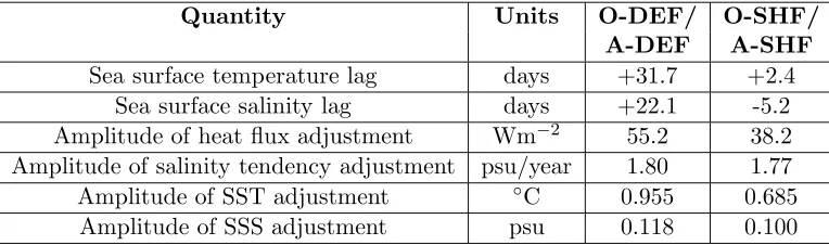
Figure 4.7 shows the lags of maximum correlation between the sea surface tem-peratures and salinities diagnosed from run O-SHF, and the World Ocean Atlas 1998 values (not the phase-shifted values which were used to spin-up the model); it can be compared with the lags of maximum correlation diagnosed from run O-DEF (Figure 3.7). The phase shift in the prescribed sea surface temperatures and salin-ities has been successful in reducing the lags, with area-weighted global-mean time lags of +2.4 and -5.2 days for the SST and SSS respectively, as opposed to +31.7 and +22.1 days for run O-DEF.
116 CHAPTER 4. MODIFIED SURFACE TRACERS
Quantity Units O-DEF/ O-SHF/ A-DEF A-SHF
Sea surface temperature lag days +31.7 +2.4 Sea surface salinity lag days +22.1 -5.2 Amplitude of heat flux adjustment Wm−2
55.2 38.2 Amplitude of salinity tendency adjustment psu/year 1.80 1.77 Amplitude of SST adjustment ◦C 0.955 0.685
[image:15.595.134.516.108.221.2]Amplitude of SSS adjustment psu 0.118 0.100
Table 4.3: Some area-weighted global-mean statistics for Mk3L ocean and atmo-sphere model runs O-DEF/A-DEF and O-SHF/A-SHF. Surface fields are diagnosed from the final 100 years of runs O-DEF and O-SHF, and from the final 40 years of runs A-DEF and A-SHF.
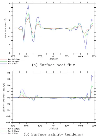
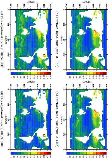
annual cycles. Figures 4.8c and 4.8d show the amplitudes of the annual cycles in the heat flux adjustments. They are generally much smaller in the case of runs O-SHF/A-SHF, confirming the hypothesis that the magnitude of the flux adjustments can be reduced by reducing the time lag between the ocean model climate and observations.
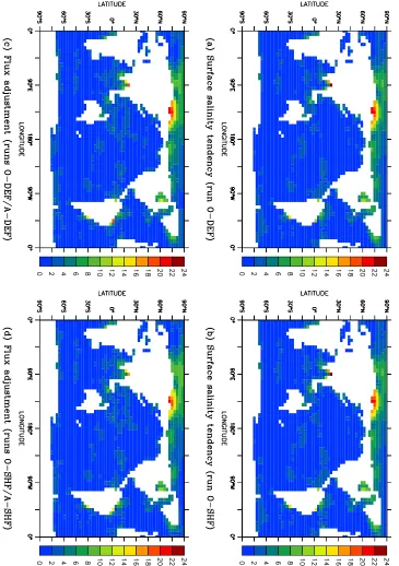
Figure 4.9 shows the amplitudes of the annual cycles in the surface salinity tendencies, and in the salinity tendency adjustments. The amplitudes of the surface fluxes can be seen to be negligibly different between the two ocean model runs. However, the reduction in the amplitudes of the flux adjustments is much smaller than in the case of the surface heat flux. This can be attributed to the lack of spatial correlation between the surface salinity tendencies simulated by the stand-alone atmosphere and ocean models, in which case a phase shift in the ocean model salinity tendencies will have little impact upon the magnitude of the flux adjustments.
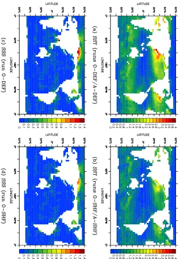
The amplitudes of the annual cycles in the sea surface temperature (SST) and sea surface salinity (SSS) adjustments are shown in Figure 4.10. By reducing the phase lag between the observed and simulated SST, the magnitude of the SST adjustments is reduced over much of the surface of the ocean. In contrast, there is a much smaller reduction in the magnitude of the SSS adjustments. This can be attributed to the generally indistinct nature of the annual cycle exhibited by the observed SSS (Section 3.5.1), and to the correspondingly poor response of the model (Section 3.3). As a result of these, a phase shift in the simulated annual cycle will have little impact upon the magnitude of the SSS adjustments.
Some global-mean statistics are shown in Table 4.3. The amplitudes of the heat flux and sea surface temperature adjustments diagnosed from runs O-SHF/A-SHF are ∼30% smaller than those diagnosed from runs O-DEF/A-DEF. The reductions in the amplitudes of the salinity tendency and sea surface salinity adjustments, however, are just 2% and 15% respectively.
4.3.4 Summary
118 CHAPTER 4. MODIFIED SURFACE TRACERS
Figure 4.8: The amplitude of the annual cycle in the surface heat flux (Wm−2
) and the heat flux adjustment (Wm−2
120 CHAPTER 4. MODIFIED SURFACE TRACERS
Figure 4.10: The amplitude of the annual cycle in the sea surface temperature (SST) adjustment (◦C) and the sea surface salinity (SSS) adjustment (psu): (a),
observations has been reduced. As a result, there has also been a reduction in the magnitude of the flux adjustments diagnosed for use within the coupled model.
4.4
Effective surface tracers
In Section 3.3, three distinct errors in the simulated sea surface temperature (SST) and sea surface salinity (SSS) were identified:
• an error in the annual mean
• an error in the amplitude of the annual cycle
• a phase lag between the simulated and observed fields
In the previous section, it was shown that the phase lag could be addressed by simply shifting the prescribed SST and SSS forward in time relative to observations. It was therefore attempted to extend this approach, to address the errors in the annual means and in the amplitudes of the annual cycle.
Consider the equilibrium response of the model. Let the observed SST (or SSS) have the annual-mean value Tobs, and let the amplitude of the annual cycle be aobs. Let the SST (or SSS) which was prescribed as the boundary condition on the model, and which may not necessarily be equal to the observed values, have the annual-mean value Tpre, and an annual cycle of amplitude apre. Let the equilibrium response of the model have annual-mean value Tmod, and an annual cycle of amplitude amod. The errors in the simulated annual-mean SST (or SSS), and in the simulated amplitude of the annual cycle, can therefore be expressed as
∆T = Tmod−Tobs (4.6)
r = amod
aobs
(4.7)
Not only can these two errors be diagnosed independently of the phase lag, but they can also be diagnosed independently of each other. Having diagnosed the errors, they can be used to modify the prescribed SST (or SSS) accordingly. The modified climatology will have an annual-mean value T′pre and an annual cycle of amplitude a′
pre, where these values are given by
T′pre = Tpre−∆T (4.8)
a′ pre =
1
rapre (4.9)
If the prescribed SST (or SSS) for monthnis expressed as the sum of the annual mean T, and an anomalyTn, thus:
Tn=T +Tn (4.10)
122 CHAPTER 4. MODIFIED SURFACE TRACERS
T′
n=T−∆T+ 1
rTn (4.11)
An iterative approach can therefore be developed, as follows:
1. Integrate the ocean model to equilibrium, with the prescribed SST (or SSS) at gridpoint (i, j) having annual-mean value Tpre(i, j), and with the amplitude of the annual cycle being apre(i, j).
2. From the simulated SST (or SSS), diagnose the values for the annual mean
Tmod(i, j), and for the amplitude of the annual cycle amod(i, j).
3. Diagnose the errors in the simulated SST and SSS, using Equations 4.6 and 4.7.
4. Derive modified values for the prescribed SST and SSS, using Equation 4.11.
5. Repeat Steps 1–4, until a pre-defined convergence criterion is satisfied.
The final values which are obtained for the prescribed SST and SSS can be termedeffectivesurface tracers. They will have been derived such that the simulated annual-mean SST and SSS at each gridpoint, and the simulated amplitudes of the annual cycles, will agree with observations to the greatest extent possible, given the spatial resolution of the model and the model physics.
This approach can be contrasted with that of Bi (2002), and with the limiting case of reducing the relaxation timescale to zero. Both these approaches seek to reduce the errors in the simulated SST and SSS, at each gridpoint and for each month of the year, to zero. However, the approach developed here only seeks to minimise the errors in the simulated annual-mean SST and SSS, and in the simulated amplitude of the annual cycle. It therefore avoids both the numerical instabilities which were encounted by Bi (2002), and the excessive surface fluxes which result when the relaxation timescale is reduced towards zero.
A comparison can also be made with the approach of Pierce (1996). By using the response of an ocean model to determine the amplitude and phase changes which arise as a result of the relaxation boundary condition, the internal transport of heat within the ocean is taken into account. The errors in both the simulated SST and SSS are also addressed, whilePierce (1996) only considers the SST.
4.4.1 Spinning up the model
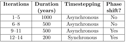
The above approach was employed to spin up the Mk3L ocean model. The spin-up procedure is summarised in Table 4.4, and consisted of the following steps:
1. The model was initialised from the end of the asynchronous stage of the default spin-up run O-DEF (Section 2.3.2).
Iterations Duration Timestepping Phase (years) shift?
1–5 1000 Asynchronous No
6–8 500 Asynchronous No
[image:21.595.196.457.107.194.2]9–11 500 Asynchronous Yes 12–14 200 Synchronous Yes
Table 4.4: A summary of the spin-up procedure for Mk3L ocean model run O-EFF.
3. The model was repeatedly integrated to equilibrium under asynchronous time-stepping. The effective surface tracers were employed as the boundary condi-tion on the sea surface temperature and salinity, while the model was forced with the same NCEP-DOE Reanalysis 2 (Kanamitsu et al., 2002) wind stresses that were used for run O-DEF. Model errors were diagnosed from the final 100 years of each iteration, and were used to derive the effective surface tracers to be used for the following iteration. The observed values for the sea surface temperature and salinity, which were used to calculate the model errors, were the same World Ocean Atlas 1998 values which were prescribed during the default spin-up run O-DEF.
4. During the iterative process, the convergence criterion for each iteration was that the rates of change in the global-mean sea surface temperature and salin-ity must be less than 0.005◦C/century and 0.001 psu/century respectively. It
was not necessary to apply these criteria to any levels other than the surface, as it was only the sea surface temperature and salinity which were required in order to calculate the model errors.
5. Five iterations of duration 1000 years were conducted, followed by three itera-tions of duration 500 years. An equilibrium solution had then been obtained, with the convergence criterion being that the differences in the global-mean potential temperature and salinity on each model level, between the final cen-turies of consecutive iterations, must be less than 0.005◦C and 0.001 psu
re-spectively. Note that all model levels were considered here, as it was desired that the final solution should represent an equilibrium solution for the ocean as a whole.
6. The final set of effective surface tracers were shifted forward in time by one month, to address the phase lag between the model and observations. The iter-ative process was then continued. A further three iterations, each of duration 500 years, were conducted, after which a fresh solution had been reached.
7. Synchronous timestepping was then employed, and the iterative process was continued, using iterations of duration 200 years. An equilibrium solution was reached after a further three iterations, representing a total of 14 iterations and 8,600 model years.
124 CHAPTER 4. MODIFIED SURFACE TRACERS
• The factor 1r, by which the amplitudes of the annual cycle in the prescribed surface tracers are multiplied from one iteration to the next, was constrained to lie within the range [0.5, 2]. This constraint was found to improve the stability of the iterative process by reducing “overshoot”, and hence to reduce the number of iterations required to reach a solution.
• To prevent the simulated sea surface temperatures from falling below the freez-ing point of seawater, the effective sea surface temperatures were constrained such that they must always be greater than or equal to -2.1◦C; this value
rep-resents the minimum sea surface temperature encountered within the World Ocean Atlas 1998 dataset. This constraint was implemented by reducing the amplitude of the annual cycle, such that the annual-minimum value of the effective sea surface temperature was equal to -2.1◦C. By reducing the
am-plitude of the annual cycle, rather than simply modifying the effective sea surface temperatures for individual months, it could be ensured that there was no change to the annual-mean sea surface temperature. This constraint was found to improve the stability of the iterative process, and to reduce the number of iterations required to reach a solution.
• No modifications were made to the prescribed surface tracers for the north-ernmost three latitude rows on the Mk3L ocean model grid, representing the region north of 79.6◦N. Within this region, the model applies a spatial Fourier
filter to the simulated tracers (Phipps, 2006), and it does not therefore respond on a gridpoint-by-gridpoint basis to external forcing. It is not therefore mean-ingful to use the gridpoint response of the model to modify the prescribed surface tracers.
• No modifications were made to the amplitude of the annual cycle in the pre-scribed sea surface salinities over the Caspian Sea, as the World Ocean Atlas 1998 sea surface salinities exhibit no annual cycle in this region.
This run shall be referred to herein as O-EFF.
In order to diagnose surface fluxes for the stand-alone atmosphere model, a 50-year atmosphere model spin-up run was also conducted. This run was identical to run A-DEF (Section 2.3.1), with the exception that the ocean currents were diagnosed from the final 100 years of run O-EFF. This run shall be referred to herein as A-EFF.
4.4.2 Convergence towards a solution
The convergence of the ocean model towards a solution is shown in Figure 4.11. Most apparent is the rapid reduction in the root-mean-square (RMS) errors in the annual-mean SST and SSS. Excluding the region north of 79.6◦N, over which the
only modification to the prescribed SST and SSS was a one-month phase shift, the RMS error in the annual-mean SST is reduced from 0.562◦C to 0.184◦C after just
one iteration. Ultimately, it is reduced to 0.007◦C, just 1.3% of the initial error.
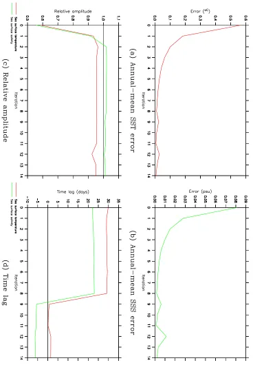
Figure 4.11: Global-mean statistics diagnosed from the final 100 years of each iter-ation of Mk3L ocean model run O-EFF: (a), (b) the root-mean-square error in the annual-mean sea surface temperature and sea surface salinity respectively, (c) the area-weighted mean relative amplitudes, and (d) the area-weighted global-mean time lags. Values north of 79.6◦N are excluded; the values plotted for Iteration
126 CHAPTER 4. MODIFIED SURFACE TRACERS
0.028 psu after just one iteration, before ultimately being reduced to 0.002 psu, just 2.4% of the initial error.
The global-mean relative amplitudes increase from 0.587 to 0.952 in the case of the SST, and from 0.558 to 1.012 in the case of the SSS. The one-month phase shift in the effective surface tracers is successful in reducing the global-mean time lags to +1.5 days and -6.2 days, in the case of SST and SSS respectively.
The fact that most of the improvement in the simulated climate is achieved after just one iteration suggests that this approach could be applied to the output of other ocean models, without the need to conduct any iterative process. The effective surface tracers diagnosed from the output of an existing spin-up run would be sufficient, when used as the boundary conditions on a further run, to significantly reduce the errors in the simulated annual-mean SST and SSS, and to considerably improve the amplitudes of the simulated annual cycles.
4.4.3 The effective surface tracers
Figure 4.12 shows the annual-mean effective surface tracers diagnosed from run O-EFF. As would clearly be expected, the modifications to the World Ocean Atlas 1998 dataset are opposite in sign to the initial errors in the simulated annual-mean SST and SSS (Figure 3.5); however, they are also comparable in magnitude, not exceeding 4.89◦C and 0.835 psu in the case of SST and SSS respectively.
Figure 4.13 shows the amplitudes of the annual cycle in the effective surface tracers, and compares them to the amplitudes of the annual cycle in the World Ocean Atlas 1998 dataset. The modifications to the amplitude of the World Ocean Atlas 1998 SST are generally small, but increase in the regions where the initial response of the model was weakest (Figure 3.6a). The amplitude is reduced at some high-latitude locations, particularly in the Southern Ocean, as a result of the constraint that the effective SST cannot be less than -2.1◦C. The modifications to
the amplitude of the World Ocean Atlas 1998 SSS are highly spatially variable, consistent with the initial response of the model (Figure 3.6b).
4.4.4 The model response
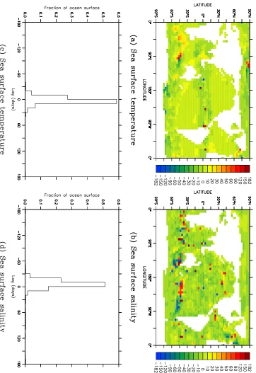
The errors in the simulated annual-mean SST and SSS, diagnosed from the final 100 years of run O-EFF, are shown in Figure 4.14. (Values for the region north of 79.6◦N, over which the only modification to the prescribed SST and SSS was a
one-month phase shift, are excluded; however the errors in the annual-mean SST and SSS do not exceed 0.87◦C and 0.48 psu respectively.) The errors can seen to
be very small, being smaller in magnitude than 0.01◦C and 0.004 psu over 92% and
97% of the surface of the ocean respectively.
The relative amplitudes are shown in Figure 4.15. North of 79.6◦N, where no
modifications were made to the annual cycles of the prescribed surface tracers, the response of the model is weak. The simulated amplitude of the annual cycle in the SST is also poor at other high-latitude locations; this arises from the suppression of the annual cycle in the effective SST, as a result of the constraint that the effective SST may not be less than -2.1◦C. Otherwise the response of the model is excellent;
Figure 4.12: The annual-mean effective sea surface temperature (SST,◦C) and sea
128 CHAPTER 4. MODIFIED SURFACE TRACERS
Figure 4.13: The amplitudes of the annual cycle in the effective sea surface tem-perature (SST,◦C) and sea surface salinity (SSS, psu) diagnosed from Mk3L ocean
Figure 4.14: The annual-mean sea surface temperature and salinity for Mk3L ocean model run O-EFF (averages for the final 100 years), expressed as anomalies relative to the World Ocean Atlas 1998: (a) sea surface temperature (◦C), and (b) sea surface
130 CHAPTER 4. MODIFIED SURFACE TRACERS
World Ocean Mk3L ocean model Atlas 1998 Run O-DEF Run O-EFF
Ross Sea 28.06 27.76 28.01
Weddell Sea 27.98 27.73 27.87
[image:28.595.111.427.107.180.2]Nordic Seas 27.96 27.72 27.88
Table 4.5: The peak surface σθ (kgm−3) in regions of deep water formation: the World Ocean Atlas 1998, and Mk3L ocean model runs O-DEF and O-EFF (averages for the final 100 years of each run). The World Ocean Atlas 1998 data has been area-averaged onto the Mk3L ocean model grid.
89% of the surface of the ocean in the case of the SST, and 96% in the case of the SSS.
The response of the model is weak at some locations in the tropics. This can be attributed, in part, to the relatively small number of iterations which were con-ducted, and particularly the fact that only three iterations were conducted under synchronous timestepping. The switch from asynchronous to synchronous timestep-ping led to some changes in the tropical climate, and three iterations appears to have been insufficient to have allowed the effective surface tracers to adapt accord-ingly. It is also possible that, at these locations, diffusive and advective processes are sufficiently strong that the surface boundary conditions have little effect upon the amplitude of the simulated annual cycle.
At other locations, the amplitude of the annual cycle in the simulated SSS is too strong, exceeding the observed amplitude even when the amplitude of the annual cycle in the effective SSS is reduced to zero. This can be attributed to an annual cycle in the fluxes of salt through the lateral walls and base of these gridboxes, in which case modification of the prescribed surface tracers is not sufficient to cause the amplitude of the simulated annual cycle to match observations.
The lags between the simulated and World Ocean Atlas 1998 SST and SSS are shown in Figure 4.16. Apart from a few locations at which the lags do not appear to have meaningful values, they are tightly clustered around zero, lying between -10 and +10 days over 95% of the surface of the ocean in the case of the SST, and 71% in the case of the SSS.
4.4.5 Densities of high-latitude surface waters
Figure 4.17 shows the peak surface water densities, as implied by the effective surface tracers, and as simulated by the Mk3L ocean model; the peak values encountered in the key regions of deep water formation are also shown in Table 4.5. The values implied by the effective surface tracers exhibit considerably greater spatial variabil-ity than those implied by the World Ocean Atlas 1998 dataset (Figure 3.1). In the Southern Hemisphere, the highest value of 29.55 kgm−3
occurs in Prydz Bay, with maximum values of 28.78 and 28.57 kgm−3
in the Ross and Weddell Seas respec-tively. In the Northern Hemisphere, the highest value of 32.63 kgm−3
occurs in Hudson Bay; the maximum value in the Nordic Seas is 28.82 kgm−3
.
132 CHAPTER 4. MODIFIED SURFACE TRACERS
134 CHAPTER 4. MODIFIED SURFACE TRACERS
World Ocean Mk3L ocean model Atlas 1998 O-DEF O-EFF Potential 0–800 m 9.61 10.88 10.15
temperature 800–2350 m 2.98 3.08 2.85
(◦C) 2350–4600 m 1.36 0.35 0.73
Salinity 0–800 m 34.75 34.69 34.78
(psu) 800–2350 m 34.68 34.50 34.68
2350–4600 m 34.74 34.46 34.69
σθ 0–800 m 26.60 26.32 26.52 (kgm−3
) 800–2350 m 27.62 27.45 27.63
2350–4600 m 27.81 27.64 27.81
Table 4.6: Global-mean potential temperature (◦C), salinity (psu), andσθ (kgm−3
): the World Ocean Atlas 1998, and Mk3L ocean model runs O-DEF and O-EFF (averages for the final 100 years of each run). The World Ocean Atlas 1998 has been volume-averaged onto the Mk3L ocean model grid.
Hemisphere of 28.01 kgm−3
in the southwestern Ross Sea, 27.95 kgm−3
in Prydz Bay and 27.87 kgm−3
in the Weddell Sea. In the Northern Hemisphere, the highest density of 27.91 kgm−3
occurs in the Barents Sea, with a maximum density of 27.88 kgm−3
in the Nordic Seas. Relative to the World Ocean Atlas 1998, the peak surface water densities in the key regions of deep water formation are too buoyant by ∼0.05–0.11 kgm−3
. While this bias can be attributed to the constraint imposed on the effective sea surface temperatures, it represents a considerable improvement on the bias of∼0.25–0.3 kgm−3
exhibited by run O-DEF (Section 3.3).
Figures 4.18, 4.19 and 4.20 show the annual cycle in sea surface temperature, salinity and density, for the deep water formation regions of the southwestern Ross Sea, western Weddell Sea and the Nordic Seas. Values are plotted for the World Ocean Atlas 1998, the effective surface tracers, and Mk3L ocean model runs O-DEF and O-EFF.
Relative to the World Ocean Atlas 1998, the amplification of the annual cycle in the effective surface tracers is apparent, as is the one-month phase shift. It is also apparent that the effective surface tracers are successful at bringing the simulated surface water properties into much better agreement with the observational values.
4.4.6 Water properties
Figure 4.21 shows the vertical profiles of potential temperature, salinity and poten-tial density, for the World Ocean Atlas 1998 and for Mk3L ocean model runs O-DEF and O-EFF. Mean values for the upper, mid- and deep ocean, as defined in Chap-ter 2, are also shown in Table 4.6. The effective surface tracers lead to significantly improved deep water properties, with the density of the deep ocean agreeing with the World Ocean Atlas 1998 to better than 0.01 kgm−3
.
136 CHAPTER 4. MODIFIED SURFACE TRACERS
Figure 4.19: The monthly-mean sea surface temperature, salinity and σθ in the western Weddell Sea, for the World Ocean Atlas 1998 (dashed red), the effective surface tracers (red), and Mk3L ocean model runs DEF (dashed green) and O-EFF (green): (a) sea surface temperature, (b) sea surface salinity, and (c) sea surface
σθ. The values plotted are the averages for the two gridpoints located at 56◦W, 72◦S, and 56◦W, 68◦S. The World Ocean Atlas 1998 data has been area-averaged onto the
Figure 4.20: The monthly-mean sea surface temperature, salinity and σθ in the Nordic (Greenland-Iceland-Norwegian) Seas, for the World Ocean Atlas 1998 (dashed red), the effective surface tracers (red), and Mk3L ocean model runs O-DEF (dashed green) and O-EFF (green): (a) sea surface temperature, (b) sea sur-face salinity, and (c) sea sursur-face σθ. The values plotted are averages for the 12 gridpoints which cover the region 14◦W–8◦E, 67◦–76◦N. The World Ocean Atlas
138 CHAPTER 4. MODIFIED SURFACE TRACERS
cold bias remains in the simulated deep ocean, the deep ocean salinities and densities are in excellent agreement with the World Ocean Atlas 1998.
The Arctic Ocean is an exception, however, remaining too warm, too fresh and too buoyant at depth. It was shown in Section 4.2 that an enhancement of ∼1 psu to the World Ocean Atlas 1998 sea surface salinities, in the presence of sea ice, led to much more realistic deep water properties in the Arctic Ocean. The failure of run O-EFF to correctly simulate the temperature and salinity of the deep Arctic Ocean, when it successfully simulates the deep water properties of the remainder of the world ocean, may further suggest that there is a “fair weather” bias in the World Ocean Atlas 1998 sea surface temperatures and salinities over the Arctic Ocean. However, this failure may also arise from the fact that, with the exception of a phase shift, no modifications were made to the prescribed surface tracers over the region north of 79.6◦N.
4.4.7 Circulation
The meridional overturning streamfunctions for the world ocean, and for the Atlantic and Pacific/Indian Oceans, are shown in Figure 4.25; they can be compared with the streamfunctions diagnosed from run O-DEF, which are shown in Figure 2.17. The increased peak surface water density in the Nordic Seas leads to an increase in the rate of North Atlantic Deep Water (NADW) formation, from 13.6 Sv for run O-DEF to 16.4 Sv for run O-EFF. As a result of the increased stratification of the water column, however, the rate of Antarctic Bottom Water (AABW) formation weakens from 9.5 to 8.5 Sv.
The rates of formation of both NADW and AABW are therefore consistent with observational estimates (Section 2.5.2).
4.4.8 Transport
The oceanic meridional transports of heat and salt, as simulated by the ocean model and as implied by the atmosphere model, are shown in Figure 4.26. The values diag-nosed from runs O-EFF and A-EFF are compared with those diagdiag-nosed from runs O-DEF and A-DEF. The increased meridional overturning in the North Atlantic leads to increased northward heat transport, bringing the simulated heat trans-ports into better agreemeent with the values implied by the atmosphere model; this indicates a reduction in the magnitude of the zonal-mean heat flux adjustments.
There is little change to the simulated oceanic salt transport, although there is better agreement with the values implied by the atmosphere model at high latitudes in the Southern Hemisphere.
4.4.9 Surface fluxes
140 CHAPTER 4. MODIFIED SURFACE TRACERS
Figure 4.22: The zonal-mean potential temperature (◦C) for the world ocean
142 CHAPTER 4. MODIFIED SURFACE TRACERS
144 CHAPTER 4. MODIFIED SURFACE TRACERS
Figure 4.27: The surface heat flux (Wm−2
146 CHAPTER 4. MODIFIED SURFACE TRACERS
Field Units Annual-mean Amplitude O-DEF/ O-EFF/ O-DEF/ O-EFF/
A-DEF A-EFF A-DEF A-EFF Heat flux Wm−2
45.2 49.4 55.2 44.4
Salinity psu/ 1.69 1.93 1.80 3.37
tendency year
SST ◦C 0.566 0.061 0.955 0.347
[image:44.595.99.441.110.220.2]SSS psu 0.082 0.014 0.118 0.089
Table 4.7: The flux adjustments diagnosed from Mk3L atmosphere and ocean model runs O-DEF/A-DEF and O-EFF/A-EFF, for the surface heat flux, surface salinity tendency, sea surface temperature (SST), and sea surface salinity (SSS): the root-mean-square annual-mean flux adjustments, and the area-weighted global-mean am-plitudes of the annual cycle in the flux adjustments. The surface fluxes are diagnosed from the final 100 years of ocean model runs O-DEF and O-EFF, and from the final 40 years of atmosphere model runs A-DEF and O-DEF.
Figure 4.28 shows the heat flux and salinity tendency adjustments diagnosed from runs O-EFF and A-EFF; these values can be compared with those diagnosed from runs O-DEF and A-DEF (Figures 2.21c and 2.22c). While there is little change to the annual-mean heat flux and salinity tendency adjustments, the amplitude of the heat flux adjustments is reduced across much of the world ocean. This was also found to occur in Section 4.3 when the phase lag between the observed and simulated sea surface temperatures was addressed. However, there is an increase in the amplitude of the salinity tendency adjustments; this can be attributed to the effective sea surface salinities having a larger amplitude than observations across much of the world ocean (Figure 4.13d).
Figure 4.29 shows the adjustments to the sea surface temperature (SST) and sea surface salinity (SSS); these values can be compared with those diagnosed from runs O-DEF and A-DEF (Figures 2.25 and 2.26). Reflecting the reductions which have been achieved in the annual-mean SST and SSS errors through the use of the effective surface tracers, the annual-mean adjustments are negligibly small across most of the world ocean. Also reflecting the improvements which have been achieved in the simulated annual cycles, both with regard to the amplitudes and the phase lags, the amplitudes of the adjustments are considerably smaller than those diagnosed from runs O-DEF and A-DEF, particularly in the case of the SST.
The root-mean-square annual-mean flux adjustments, and the global-mean am-plitudes of the annual cycles, are shown in Table 4.7, for runs O-DEF/A-DEF and O-EFF/A-EFF. The reduction in the magnitude of the SST and SSS adjustments is apparent, as is the reduction in the amplitude of the heat flux adjustments, and theincrease in the amplitude of the salinity tendency adjustments.
4.4.10 Summary
Figure 4.28: The heat flux adjustment (Wm−2
148 CHAPTER 4. MODIFIED SURFACE TRACERS
Figure 4.29: The sea surface temperature adjustment (◦C) and sea surface salinity
salinities, and the simulated amplitudes of the annual cycles, agree with observations to the greatest extent possible. A considerable improvement in the simulated ocean climate is obtained, with a realistic vertical density profile and rates of deep water formation that are consistant with observational estimates.