Investigating acoustic propagation in gassy marine sediments using a bubbly gel mimic

Investigating Acoustic Propagation in Gassy Marine Sediments using a Bubbly Gel Mimic

G.B.N. Robb, T.G. Leighton, V.F. Humphrey, A.I. Best, J.K. Dix and Z. Klusek

SCIENTIFIC PUBLICATIONS BY THE ISVR

Technical Reports are published to promote timely dissemination of research results by ISVR personnel. This medium permits more detailed presentation than is usually acceptable for scientific journals. Responsibility for both the content and any opinions expressed rests entirely with the author(s).

Technical Memoranda are produced to enable the early or preliminary release of information by ISVR personnel where such release is deemed to the appropriate. Information contained in these memoranda may be incomplete, or form part of a continuing programme; this should be borne in mind when using or quoting from these documents.

Contract Reports are produced to record the results of scientific work carried out for sponsors, under contract. The ISVR treats these reports as confidential to sponsors and does not make them available for general circulation. Individual sponsors may, however, authorize subsequent release of the material.

COPYRIGHT NOTICE

(c) ISVR University of Southampton All rights reserved.

UNIVERSITY OF SOUTHAMPTON

INSTITUTE OF SOUND AND VIBRATION RESEARCH FLUID DYNAMIC AND ACOUSTICS GROUP

Investigating Acoustic Propagation in Gassy Marine Sediments Using a Bubbly Gel Mimic

by

G.B.N. Robb, T.G. Leighton, V.F. Humphrey, A.I. Best, J.K. Dix and Z. Klusek

ISVR Technical Report No. 315

July 2007

ACKNOWLEDGMENTS

Contents Page

Acknowledgements ii

Contents iii

List of figures and tables iv

Abstract v

List of abbreviations vi

List of symbols vii

I Introduction 1

II Experiment 6

III Results and Discussion 8

IV Conclusions 10

References

LIST OF FIGURES AND TABLES PAGES

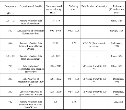
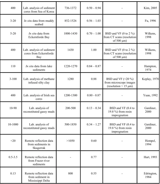
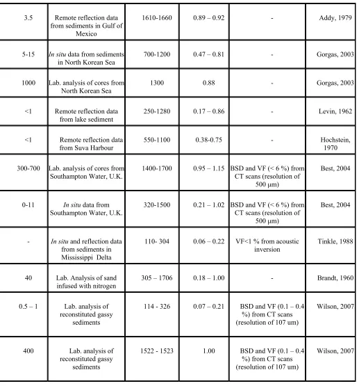
Table 1 Compilation of measured compressional wave velocities of gassy sediments, including: frequency (kHz), experimental technique and sediment under examination, compressional wave velocity (m.s-1_),

ratio of velocity in gassy sediment to that in saturated sediment, available information on bubble population and reference. Note that the symbol – indicates that no available information is available.

2-4

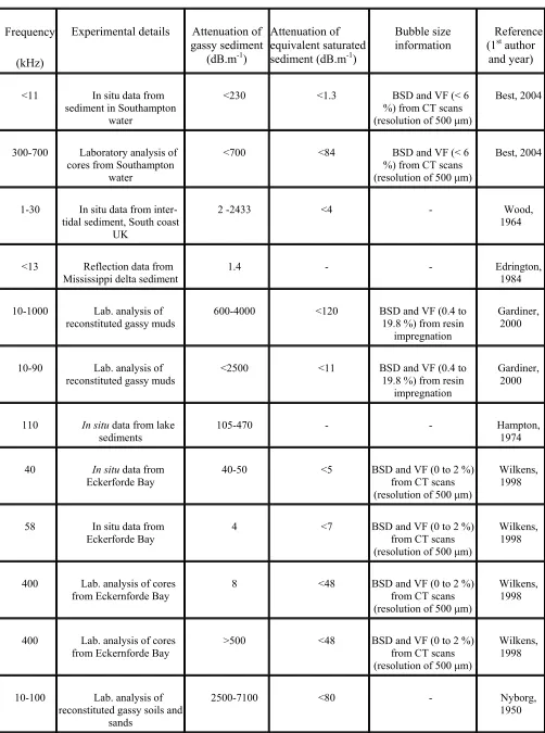
Table 2 Table 2: Compilation of measured compressional wave attenuations of gassy sediments, including: frequency (kHz), experimental technique and sediment under examination, compressional wave attenuation of gassy sediment (dB.m-1), predicted compressional wave attenuation of equivalent saturated sediment (dB.m-1), available information on bubble population and reference. Note that the symbol - indicates that no available information is available and that the attenuation α of the saturated sediment was obtained from the frequency f using α=kf, where the constant of proportionality k was obtained from Hamilton (1972).

5-6

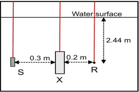
Figure 1 Experimental setup, showing relative positions of source S, xanthan sample X and receiver R at common depth of 2.44 m and separations of 0.3 m and 0.2 m respectively. All devices were

deployed on carbon rods (denoted by vertical lines) to

allow relative positions to be accurately obtained.

6

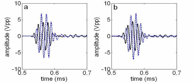
Figure 2 Example received signals at central frequency of 65 kHz, including a single, unprocessed signal (a) and the output of the processing stage (i.e. after the application of band-pass filtering and the stacking of 50 shots). Reference signals are displayed as dashed line, while the sample signals are displayed as solid lines.

7

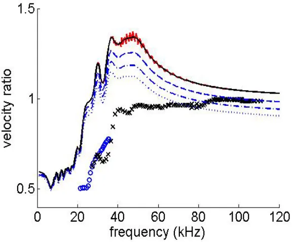
Figure 3 Measured and predicted velocity ratios. Measured velocity ratios are displayed for LF source (circles) and HF source (crosses). The predicted ratio of phase velocity in bubbly gel to that in bubble-free gel are shown for the best-fit population using 2.5 µm bins (oscillatory solid line) and 0.5 µm bins (smooth solid line). Predicted ratios are also shown for this best-fit population, using 0.5 µm bins, with additional Gaussian contributions added from 5 to 20 µm with void fractions of 1.7x10-3 (dash line), 3.5x10-3 (dotted line) and 5.1x10-3 % (dash-dot line).

8

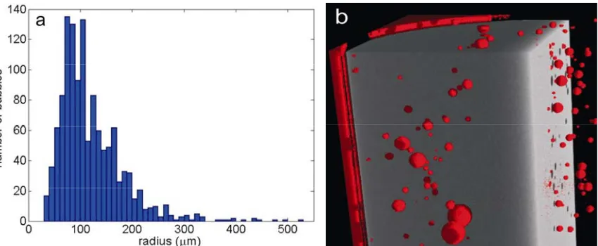
Figure 4 Measured bubble distribution, including: (a) combined bubble distribution obtained from the three sub-samples and (b) a 3-D CT image of a vertical segment of one of the cylindrical samples, with the host gel clipped back to allow the bubbles to be more clearly observed.

ABSTRACT

The acoustic techniques available for the determination of bubble size distributions in fluids are presently more sophisticated than those available for gassy sediments. To provide a simplified platform for the testing of models for acoustic propagation in marine sediments, experiments have been performed on a bubbly gel mimic. This eliminates the granular and inhomogeneous nature of the host medium. Compressional wave velocities are measured in a bubbly xanthan gel sample from 21 to 111 kHz. In the frequency range of 25 to 40 kHz, these display a sharp transition between the lower and upper asymptotic values of the velocity ratio. Bubble size distributions measured using CT scanning techniques possess modal radii from 70 to 110 µm, radii whose resonant frequencies directly correspond to the frequency range over which the sharp transition occurs. Velocity ratios predicted by the Anderson and Hampton acoustic theory for gassy sediments differ considerably from measured values, with the gel effectively acting as a fluid with negligible shear modulus. Predicted values are very sensitive to both the size of the radii bins used and the inclusion of bubbles with radii too small to be detected by the CT scanner, i.e. those bubbles having radii less than 30 µm.

LIST OF ABBREVIATIONS

BSD: Bubble Size Distribution CT: Computed Tomography D/A: Digital to Analogue

LF: Low Frequency

HF: High Frequency

LIST OF SYMBOLS

α Compressional wave attenuation (dB.m-1)

d Sample thickness (m)

∆t Difference in arrival time between samples and reference signal (s)

f Frequency (Hz)

fo Reference frequency (1 Hz)

G Shear modulus (Pa)

K Bulk modulus (Pa)

k constant of proportionality (dB.m-1.kHz-1) ρ Bulk density (kg.m-3)

r Bubbles radius (m)

tC time correction for Perspex walls (s)

v Compressional wave velocity (m.s-1)

vr Compressional wave velocity ratio (dimensionless)

vw compressional wave velocity of water (m.s-1)

I. Introduction.

Regions of seafloor sediments that contain gas bubbles, primarily methane, have been identified at numerous global locations (Fleischer et al., 2001). These have been detected primarily through the significant impact of the bubbles on the bulk acoustic properties of the sediment, with typical “gassy” features observed on high-resolution seismic profiles including acoustic turbidity and blanking (Judd and Hovland, 1992). These features arise from the large and strongly frequency-dependent acoustic cross-section that each bubble presents to the insonifying sound field (Anderson and Hampton, 1980a, b).

It would be beneficial to a number of marine applications if the existing acoustic capability to identify the spatial extent of gassy sediments could be extended to allow either the bubble size distributions (BSDs) or void fractions (VF) to be measured. First, the increased understanding of the acoustic properties of gassy sediments required to obtain measurements of BSDs from acoustic signals would greatly assist marine surveyors, possibly allowing the interpretation of previously disrupted regions on seismic profiles. Second, the bubble distribution will affect the shear strength and load-bearing capacity of the sediment (Sill et al. 1991; Wheeler and Gardiner 1989) and will therefore be of interest to offshore geohazard assessment. Third, the flux of methane from the seabed to the atmosphere, of which climate modellers require more refined information (Judd, 2003), will depend on the BSDs present in the sediment.

The ability for a user to be able to determine BSDs quantitatively depends on the level of sophistication of both the acoustic measurement techniques and the acoustic theories available for inverting acoustic data obtained by these techniques. In comparison to water-based bubble populations, where non-linear, non-stationary acoustic theories have been developed (Leighton, 2004, 2005; Leighton et al., 2004), the existing theories for sediment-based bubble populations are limited to linear stationary scenarios (Anderson and Hampton, 1980a, b). Similarly, advanced acoustic measurement techniques, such as the analysis of non-linear sum and difference signals (Leighton, 2004), are at a more advanced stage for water-based than sediment-based bubble populations.

While the more developed nature of the water-based measurements and theories can be partly attributed to their numerous industrial, medical and oceanographic applications (Leighton, 1997), the uniform, homogeneous nature of the media containing the bubbles is also a factor. In contrast to the fundamental properties of water (e.g. velocity and density) which can be determined using standard predictive equations (Siedler, 1986), the fundamental properties of the saturated sediment component of gassy sediments are difficult to predict. Recent work has identified that compressional wave velocities in sediments of the same sedimentological classification and depth, with similar porosities (variations of less than 1 %) and which are located within lateral distances of order 100 m can vary by up to 10 % (Robb et al., 2006), a value which agrees with previous research in this field (Hamilton, 1987). In addition to this variability, which is attributed to the subtle differences in structure and grain size distribution of the sediment (Robb et al., 2007; Hamilton 1987), the ability of marine sediments to support shear forces adds a further level of complexity to the bubble host medium.

for gassy sediments. The pre-dominant technique used to independently measure bubble populations is X-Ray CT scanning, which until recently was limited to the use of medical CT scanners with spatial resolutions of 500 µm. The recent advancement of CT scanning technologies to reduce spatial resolution to the order of 10s µm (Reed and Briggs, 2003) provides a great resource with which knowledge of bubble populations in gassy sediments, and acoustic theories, can be improved.

It would therefore be useful to measure the acoustic properties of bubbly media in which the host media is homogeneous and supports shear, e.g. water-based gels, and compare these to bubble populations obtained using high-resolution CT scanners. This report presents such a comparison for a bubbly xanthan gel and also investigates the applicability of the state-of-the-art sediment-based acoustic model of Anderson and Hampton (1980a, b) to this media.

Frequency

(kHz)

Experimental details Compressional wave velocity

(m.s-1₎

Velocity ratio

Bubble size information Reference

(1st _{author and}

year)

0.6 – 1.2 Remote reflection data

from lake sediment 75 – 170 - - Jones, 1958

500 Lab. analysis of cores from

Eckernforde Bay 900 - 1460 0.62 – 1.00 - Slowey, 1996

<0.4 Remote reflection data from sediment offshore

Oregon

1250 0.70 VF≈2 % (from acoustic

inversion) Andreassen, 1997

0.2 – 3.2 Remote reflection data from lake sediment

45 - 122 - - Jones, 1964

700 Lab. analysis of reconstituted sand at range

of pressures

1264 - 2515 - VF varied from 0 to 100

% Elliot, 1975

200 Lab. Analysis of reconstituted sand at 1500

psi

1254 - 2072 0.61 – 1.00 VF varied from 0 to 100 %

Domenico, 1976

200 Laboratory analysis of glass beads at 1500 psi

1218 - 2090 0.58 – 1.00 VF varied from 0 to 100 %

Domenico, 1977

<12 Remote reflection data from sediment in South

Sea of Korea

800 0.55 - Lee, 2005

Table continued on next page Table continued from previous page

400 Lab. analysis of sediment

cores from Sea of Korea 736-1372 0.50 – 0.94 - Kim, 2005

3-20 In situ data from muddy seabed

852-1526 0.56 – 1.03 - Fu, 1996

5-20 In situ data from

Eckernforde Bay 1000-1430 0.70 – 1.00 from CT scans (resolution BSD and VF (0 to 2 %) of 500 µm)

Wilkens, 1998

400 Lab. analysis of sediment cores from Eckernforde

Bay

1430 1.00 BSD and VF (0 to 2 %) from CT scans (resolution

of 500 µm)

Wilkens, 1998

110 In situ data from lake

sediments 1220-1270 0.84 – 0.87 - Hampton, 1974

3-100 Lab. analysis of methane

infused silty clay 1280 0.88 from microscope images BSD and VF (<20 %) (resolution > 15 µm)

Keplay, 1978

400 Lab. analysis of Irish sea cores

1200-1300 0.80 - 0.87 - Yuan, 1992

10-90 Lab. analysis of

reconstituted gassy muds 200-500 0.13 – 0.34 19.8 %) from resin BSD and VF (0.4 to impregnation

Gardiner, 2000

10-1000 Lab. analysis of

reconstituted gassy muds 500-1850 0.34 – 1.27 19.8 %) from resin BSD and VF (0.4 to impregnation

Gardiner, 2000

<20 Remote reflection data from sediments in

Skagerrak

>1050 0.60 - Hempel,

1994

0.5-3.5 Remote reflection data from Frazer river

sediments

- 0.77 - Hart, 1993

0.13 Remote reflection data from sediment in Mississippi Delta

800 0.55 - Edrington,

1984

Table continued on next page

3.5 Remote reflection data from sediments in Gulf of

Mexico

1610-1660 0.89 – 0.92 - Addy, 1979

5-15 In situ data from sediments

in North Korean Sea 700-1200 0.47 – 0.81 - Gorgas, 2003

1000 Lab. analysis of cores from

North Korean Sea 1300 0.88 - Gorgas, 2003

<1 Remote reflection data from lake sediment

250-1280 0.17 – 0.86 - Levin, 1962

<1 Remote reflection data

from Suva Harbour 550-1100 0.38-0.75 - Hochstein, 1970

300-700 Lab. analysis of cores from Southampton Water, U.K.

1400-1700 0.95 – 1.15 BSD and VF (< 6 %) from CT scans (resolution of

500 µm)

Best, 2004

0-11 In situ data from

Southampton Water, U.K. 320-1500 0.21 – 1.02 BSD and VF (< 6 %) from CT scans (resolution of 500 µm)

Best, 2004

- In situ and reflection data from sediments in Mississippi Delta

110- 304 0.06 – 0.22 VF<1 % from acoustic

inversion Tinkle, 1988

40 Lab. Analysis of sand

infused with nitrogen 305 – 1706 0.18 – 1.00 - Brandt, 1960

0.5 – 1 Lab. analysis of reconstituted gassy

sediments

114 - 326 0.07 – 0.21 BSD and VF (0.1 – 0.4 %) from CT scans (resolution of 107 um)

Wilson, 2007

400 Lab. analysis of reconstituted gassy

sediments

1522 - 1523 1.00 BSD and VF (0.1 – 0.4 %) from CT scans (resolution of 107 um)

Wilson, 2007

Table 1: Compilation of measured compressional wave velocities of gassy sediments, including: frequency (kHz), experimental technique and sediment under examination, compressional wave velocity (m.s-1), ratio of velocity in gassy sediment to that in saturated sediment, available information on bubble population and reference. Note that the symbol – indicates that no available information is available.

Frequency

(kHz)

Experimental details Attenuation of gassy sediment

(dB.m-1)

Attenuation of equivalent saturated sediment (dB.m-1)

Bubble size information

Reference (1st _author

and year)

<11 In situ data from sediment in Southampton

water

<230 <1.3 BSD and VF (< 6 %) from CT scans (resolution of 500 µm)

Best, 2004

300-700 Laboratory analysis of cores from Southampton

water

<700 <84 BSD and VF (< 6 %) from CT scans (resolution of 500 µm)

Best, 2004

1-30 In situ data from inter-tidal sediment, South coast

UK

2 -2433 <4 - Wood,

1964

<13 Reflection data from

Mississippi delta sediment 1.4 - - Edrington, 1984

10-1000 Lab. analysis of

reconstituted gassy muds 600-4000 <120

BSD and VF (0.4 to 19.8 %) from resin

impregnation

Gardiner, 2000

10-90 Lab. analysis of reconstituted gassy muds

<2500 <11 BSD and VF (0.4 to 19.8 %) from resin

impregnation

Gardiner, 2000

110 In situ data from lake

sediments 105-470 - - Hampton, 1974

40 In situ data from

Eckerforde Bay 40-50 <5

BSD and VF (0 to 2 %) from CT scans (resolution of 500 µm)

Wilkens, 1998

58 In situ data from Eckerforde Bay

4 <7 BSD and VF (0 to 2 %) from CT scans (resolution of 500 µm)

Wilkens, 1998

400 Lab. analysis of cores

from Eckernforde Bay 8 <48 BSD and VF (0 to 2 %) from CT scans (resolution of 500 µm)

Wilkens, 1998

400 Lab. analysis of cores

from Eckernforde Bay >500 <48 BSD and VF (0 to 2 %) from CT scans (resolution of 500 µm)

Wilkens, 1998

10-100 Lab. analysis of reconstituted gassy soils and

sands

2500-7100 <80 - Nyborg,

1950

Table continued from previous page

40-80 In situ data from gassy

muds 25-90 <10 - Anderson, 1980a

40 In situ data from gassy

muds 13 <5 - Anderson, 1980a

Table 2: Compilation of measured compressional wave attenuations of gassy sediments, including: frequency (kHz), experimental technique and sediment under examination, compressional wave attenuation of gassy sediment(dB.m-1), predicted compressional wave attenuation of equivalent saturated sediment (dB.m-1), available information on bubble population and reference. Note that the symbol - indicates that no available information is available and that the attenuation α of the saturated sediment was obtained from the frequency f using α=kf, where the constant of proportionality k was obtained from Hamilton (1972).

II. Experiment

Propagation experiments were performed on samples of xanthan gel which were confined in a Polymethylmethacrylate (Perspex) box measuring 96 mm x 280 mm x 580 mm. This was suspended co-linearly along a horizontal axis with the required sources and receiver (as displayed in Fig. 1) in a large water tank, which measured 8 m x 8 m x 5 m deep. To span a wide frequency range two custom-made high-fidelity sources, developed by Neptune Sonar Ltd. and Blacknor Technology Ltd., were used. These included a low-frequency (LF) source which operates from 21 to 36 kHz and a high-frequency (HF) source which operates from 27 to 111 kHz. In order to achieve accurate positioning, all devices were deployed using purpose built carbon rods which were firmly attached to cross-bars across the top of the tank. The separation between the source and the sample (0.3 m) minimises beam spreading at the sample face (and therefore minimises the magnitude of diffractions and reflections from the box edges) while ensuring that the sample lies beyond the near-field to far-field transition of the sources (greater than 0.27 m for both sources). The position of the receiver also maximises the time difference between the diffraction and reflection events and the direct arrival, a factor which becomes more important at lower frequencies.

Figure 1: Experimental setup, showing relative positions of source S, xanthan sample X and receiver R at common depth of 2.44 m and separations of 0.3 m and 0.2 m respectively.

All devices were deployed on carbon rods (denoted by vertical lines) to allow relative positions to be accurately obtained.

A xanthan gel, with a concentration by weight of 2 %, was selected as the host medium for the bubbles, owing to its ability to support bubble populations of a similar size to those observed in gassy sediments in nature, i.e. radii from 10s of µm to 10 mm (see review by Robb et al., 2006). As these populations remain stable over periods of the order of 2 to 4.5 hours for 0.8 % concentration gels (Hwang et al., 1995), it is assumed that the bubbles present in the 2 % gel remain stable over the 6 hour period required to perform the acoustic measurements described here.

Initially bubble-free samples of the xanthan gel were produced in a saline solution (35 ‰). The preparation of these samples at a water temperature of approximately 40 to 50 oC slowed the setting rate sufficiently to allow a homogeneous mixture of gel to form without the need for rapid stirring, a process which intrinsically introduces bubbles. Using the experimental arrangement in Fig. 1 the compressional wave group velocity of the bubble free gel was measured to be 1565 m·s-1 + 10 m·s-1, while the bulk density ρ of the bubble-free gel was independently measured to be 999 kg·m-3 + 10 kg·m-3. Additional portions of this gel were then whisked to introduce air bubbles with a wide range of sizes (radii from 10s of µm to cms). Bubbles with sizes broadly relevant to the frequency range under examination,i.e. radii of order 10s to 100s of µm, were then selected using a syringe with an aperture of order 200 µm and injected at discrete points into the bubble-free gel. The sample was then capped underwater to prevent the trapping of any large air voids. To obtain a measure of the BSD, three 5 ml sub-samples of bubbly gel were collected prior to the propagation experiments. These were immediately analysed using a X-Tek CT scanner, which uses the attenuation of X-rays to map the density composition of a material. The image resolution of each scan, which depends on the size of the sample and its position in the scanner, ranged from 12.1 to 12.8 µm for the three sub-samples examined.

Pulses containing three oscillations, with central frequencies ranging from 20 to 111 kHz in 1 kHz steps were generated using a D/A card with a 1 MHz sampling rate. These were transmitted through a matched power amplifier to the relevant source, with fifty shots acquired at each central frequency. Group velocities were obtained through the comparison of signals that had propagated through the bubbly gel sample with reference signals received without the sample present. Between these two sets of measurements the source and receiver were unmoved. In each case the received signals were stacked and filtered, using 3rd order Butterworth band-pass filters with band-pass-bands that scaled to account for the change in the bandwidth of the signals across the frequency band examined. Example reference (water-based) and sample signals are displayed in Fig. 2.

Figure 2: Example received signals at central frequency of 65 kHz, including a single, unprocessed signal (a) and the output of the processing stage (i.e. after the application of

The time difference ∆t between the sample signal and the reference signal was then determined from the maximum of the cross-correlation of the signal envelopes, with the envelopes computed using the Hilbert transform. The velocity v was calculated using:

C

W d v

d

t t _v

=

⎛_{∆ − +} ⎞

⎜ ⎟

⎝ ⎠

(1),

where d is the thickness of the sample and tC is the time correction required to account for the

insertion of the sample box (which introduces two 1 mm thick Perspex walls). Errors in the velocity, which range from 1.3 to 1.7 %, were obtained by propagating the timing resolution of the acquisition system (+ 0.5 µs) and the uncertainties in the sample thickness (+ 1 mm) through Equation 1.

III. Results and discussion.

The measured velocity ratios (see Figure 3) were obtained by dividing the measured group velocity by the velocity of the bubble-free gel. Velocity ratios appear to be relatively independent of frequency from 21 to 25 kHz and 40 to 111 kHz. A steep increase is observed in velocity ratio as frequency increases from 25 to 40 kHz with a strong agreement observed between the values determined from the two different sources.

Figure 3: Measured and predicted velocity ratios. Measured velocity ratios are displayed for LF source (circles) and HF source (crosses). The predicted ratio of phase velocity in

bubbly gel to that in bubble-free gel are shown for the best-fit population using 2.5 µm bins (oscillatory solid line) and 0.5 µm bins (smooth solid line). Predicted ratios are also

shown for this best-fit population, using 0.5 µm bins, with additional Gaussian contributions added from 5 to 20 µm with void fractions of 1.7x10-3 (dash line), 3.5x10-3

(dotted line) and 5.1x10-3 % (dash-dot line).

The combined number of bubbles measured in the sub-samples (Figure 4(a)) is dominated by radii r from 70 to 110 µm. The spherical nature of these bubbles is displayed in a 3-D volume from one of the samples (Figure 4(b)). The resonant frequencies fr of the modal radii

were estimated, through the use of fr·r=3 Hz·m (Leighton, 1997), to vary from 27 to 43 kHz. These values correspond well with the frequency range over which highly dispersive group velocities are measured. As the bubble population was observed to be strongly heterogeneous, the results of the CT scans can only be used to determine the BSD of the bulk sample. The void fraction was estimated to be 0.05 %, from the approximate volume of bubbles injected into the bubble-free sample. Note that no information could be obtained concerning bubbles with radii less than 30 µm, as these could not be detected above noise in the CT data.

Figure 4: Measured bubble distribution, including: (a) combined bubble distribution obtained from the three sub-samples and (b) a 3-D CT image of a vertical segment of one of the cylindrical samples, with the host gel clipped back to allow the bubbles to be more clearly observed.

The acoustic theory of Anderson and Hampton (1980a, b) was used to predict the phase velocity of the bubbly gel. While this theory was developed for gassy marine sediments, through the incorporation of shear-based terms into the fluid-based theory of Silberman (1957), it can be applied to any gassy medium in which the host medium possesses a finite shear modulus. The key parameters in this model are the BSD, which has been measured, and the bulk modulus K and shear modulus G of the host material.

A detailed examination of the extant literature revealed no values for the bulk and shear modulus of xanthan gel at the frequencies of interest to this work. The shear modulus was therefore obtained by extrapolating shear moduli measurements made on xanthan gel, at concentration of 4 %, from 160 mHz to 16 Hz (Hyun et al., 2002). These can be expressed in term of the frequency f using the following power law relationship:

152 . 0

132 _⎟

⎠ ⎞ ⎜ ⎝ ⎛ ⋅ =

o f f

G (2),

where fo is 1 Hz. The extrapolation of this relationship to the kHz frequencies examined in this work produces an upper limit on the shear modulus of 800 Pa, which is three to four orders of magnitude less than the shear modulus of marine muds and five to six orders less than that of marine sands (Hamilton, 1971) at similar frequencies. The bulk modulus of the gel was then calculated using:

ρ

G K

v= +43 (3).

Equation 3 and can be omitted. The measured velocity (1565 m·s-1) and bulk density (999 kg·m-3) of the bubble-free gel give a bulk modulus of 2.45 GPa.

The measured bubble sizes were interpolated to 0.5 µm bins, as coarser bin size resulted in artefacts in the predicted (see Fig. 3). It is interesting to note that the low values of shear modulus effectively removes any dependence of the model on shear, reducing the Anderson and Hampton model to the fluid based theory (Spitzer, 1943; Silberman, 1957) from which it was derived. The void fraction was then adjusted to obtain a best-fit bubble population, with the resulting void fraction (0.013 %) approximately ¼ that of the estimated void fraction. This was achieved by fitting the upper and lower limits of the predicted phase velocity to corresponding plateaus in the measured group velocity There are however notable discrepancies between the predicted and measured values, in both the frequency range over which the transition from low to high velocity ratios occurs and the overall over-prediction of measured velocity ratios.

One possible explanation for the difference in the measured and predicted velocity ratios is that bubbles with radii less than 30 µm may be present. Tests indicated that the inclusion of additional Gaussian distributions which spanned radii from 5 to 20 µm acted to reduce the magnitude of the predicted velocity ratios from 20 to 80 kHz, without modifying the lower limit present at lower frequencies. Typical results are displayed in Fig. 3 for modified populations, which consist of the best-fit population, with a void fraction of 0.013 %, and additional Gaussian components from 5 to 20 µm with void fractions from 1.7x10-3 and 5.1x10-3 %.

Even with the inclusion of smaller unresolvable bubbles, the predicted velocity ratios differ considerably from the measured values. This may be a consequence of the comparison of predicted phase velocities with measured group velocities. These will differ for frequencies whose pulses possess bandwidth which extend into the measured range of dispersive velocities, namely pulses with central frequencies from 21 to 60 kHz. An alternative explanation is the linear nature of the model used, while the actual pressures that impinge on the sample are predicted to be 5 to 25 kPa (from known source levels, amplifier gains and beam patterns) and are likely to require the inclusion of non-linear effects (Leighton et al., 2004).

IV. Conclusions

The compressional wave velocity of a bubbly xanthan gel sample was measured over the frequency range of 21 to 111 kHz. The velocity ratio between the bubbly gel and bubble-free gel displays a sharp transition between lower and upper asymptotes at frequencies between 25 to 40 kHz. The bubble size distribution measured using CT scanning techniques displays modal radii between 70 and 110 µm, the resonant frequencies of which directly correspond to the sharp transition in velocity ratio. The velocity ratios predicted by the acoustic theory of Anderson and Hampton [3,4] differ considerably from measured values, with the xanthan gel effectively acting as a fluid. The inclusion of bubbles with radii less than 20 µm, i.e. those undetectable above the noise in the CT data, has a considerable effect on the predicted velocity ratios. The objectives of future work include the use of CT scanning to determine the long-term stability of bubble populations in the xanthan samples and the measurement of the phase velocity, as described Sachse and Pao (1978), to allow direct comparison of measured and predicted velocity ratios.

References

Addy, S.K. and Worzel, J.L., 1979, Gas seeps and subsurface structure off Panama city, Florida, American Association of Petroleum Geologists Bulletin, 63, 668-675.

Andreassen, K., Hart, P.E. and MacKay, M., 1997, Amplitude versus offset modelling of the bottom stimulated reflection associated with submarine gas hydrates, Marine Geology, 137(1-2), 25-40.

Anderson, A.L. and Hampton, L.D., 1980a, Acoustics of gas bearing sediments I, Background, Journal of the Acoustical Society of America, 67(6), 1865-1889.

Anderson, A.L. and Hampton, L.D., 1980b, Acoustics of gas bearing sediments II. Measurements and models, Journal of the Acoustical Society of America, 67(6), 1890-1903. Best, A.I., Tuffin, M.D.J, Dix, J.K. and Bull, J.M., 2004, Tidal height and frequency dependence

of acoustic velocity and attenuation in shallow gassy marine sediments, Journal of Geophysical Research, 109, B08101

Brandt, H., 1960, Factors affecting compressional wave velocities in unconsolidated marine sand sediments, Journal of the Acoustical Society of America, 32(2), 171-179.

Domenico, S.N., 1976, Effect of brine-gas mixture on velocity in an unconsolidated sand reservoir, Geophysics, 41(5), 882-894.

Domenico, S.N., 1977, Elastic properties of unconsolidated porous sand reservoirs, Geophysics, 42(7), 1339-1368.

Edrington, T.S. and Calloway, T.M., 1984, Sound speed and attenuation measurements in gassy sediments in the Gulf of Mexico, Geophysics, 49(3), 297-299.

Elliot, S.E. and Wiley, B.F., 1975, Compressional velocities of partially saturated unconsolidated sands, Geophysics, 40(6), 949-954.

Fleischer, P., Orsi, T.H., Richardson M.D. and Anderson A.L., 2001, Distribution of free gas in marine sediments: a global overview, Geo-Marine Letters, 21, 103-122.

Fu, S.S., Wilkens, R.H. and Frazer, L.N., 1996, In situ velocity profiles in gassy sediments: Kiel Bay, Geo-Marine Letters, 16, 249-253.

Gardiner, T.N., 2000, An acoustic study of soils that model seabed sediments containing gas bubbles, Journal of the Acoustical Society of America, 107(1), 163-176.

Gorgas, T.J., Wilkens, R.H., Shung, S.F, Frazer, L.N., Richardson, M.D., Briggs, K.B. and Lee, H., 2002, In situ acoustic and laboratory ultrasonic sound speed and attenuation measured in heterogeneous soft seabed sediments: Eel River shelf, California, Marine Geology, 182, 103-119.

Hamilton, E.L., 1971, Elastic properties of marine sediments, Journal of Geophysical Research,

76(2), 579-603.

Hamilton, E.L., 1972, Compressional-wave attenuation in marine sediments, Geophysics, 37(4), 620-646.

Hamilton, E.L., 1987, Acoustic properties of sediments, In Acoustics and the ocean bottom, A Lara-Saenz, C Ranz-Guerra and C Carbo-Fite, CSIS Madrid, 4-58.

Hart, B.S. and Hamilton, T.S., 1993, High-resolution acoustic mapping of shallow gas in unconsolidated sediments beneath the strait of Geogia, British Columbia, Geo-Marine Letters, 13, 49-55.

Hampton, L.D., and Anderson, A.L., 1974, in “Natural gas in marine sediments”, Ed. Kaplan, I.R., Plenum Press, New York,

Hempel, P., Spiess, V. and Schreiber, R., 1994, Expulsion of shallow gas in the Skagerrak- Evidence from subbotton profiling, seismic, hydroacoustic and geochemical data, Estuarine Coastal and Shelf Science, 38(6), 583-601.

Hochstein, M.P., 1970, Seismic measurements in Suva Harbour (FIJI), New Zealand Journal of Geology and Geophysics, 13, 269-281.

Hwang, P.A., Roy, R.A. and Crum, L.A., 1995, Artificial bubble cloud targets for underwater acoustic remote sensing, J. Atmospheric and Oceanic Technology, 12, 1287-1302.

Hyun, K., Kim, S.H., Ahn, K.H., and Lee, S.J., 2002, Large amplitude oscillatory shear as a way to classify the complex fluids, Journal of Non-Newtonian Fluid Mechanics, 107, 51-65. Jones, J.L., Leslie, C.B. and Barton, L.E., 1958, Acoustic characteristics of a lake bottom,

Jones, J.L., Leslie, C.B. and Barton, L.E., 1964, Acoustic characteristics of underwater bottom, Journal of the Acoustical Society of America, 36(1), 154-157.

Judd, A.G. and Hovland, M., 1992. The evidence of shallow gas in marine sediments, Continental Shelf Research, 12(10), 1081-1095.

Keplay, P.E. and Cooke, R.C., 1978, Velocity of sound as a function of bubble distribution in gas-bearing sediments, Geophysical Research Letters, 5(12), 1071-1073.

Kim, D.C, Yeo, J.Y., Lee, G.H and Park, S.C, 2005, Seismic characteristics and physical properties of gas-bearing sediment in the Jinhae Bay, the South Sea of Korea, Proceedings to the VIII International Conference on Gas in Marine Sediments, Vigo, Spain, 185-190.

Judd, A.G., 2003. The global importance and context of methane escape from the seabed, Geo-Marine Letters, 23, 147-154.

Lee, G.H., Kim, D.C., Kim, H.J., Jou, H.T., Lee, Y.J. and Park, S.C., 2005, Shallow gas off the southeastern cost of Korea, Proceedings to the VIII International Conference on Gas in Marine Sediments, Vigo, Spain, 87-89.

Leighton, T.G., 1997, The Acoustic Bubble, Academic Press, London, 613 pp.

Leighton, T.G., 2004, From babbling brooks to baby scans, from seas to surgeries: The pressure fields produced by non-interacting spherical bubbles at low & medium amplitudes of pulsation, International Journal of Modern Physics B, 18(25), 3267-3314.

Leighton, T.G., 2005, Nonlinear Bubble Dynamics & The Effects On Propagation Through Near-Surface Bubble Layers, In High-Frequency Ocean Acoustics, MB Porter, M Siderius, & W Kuperman, American Institute of Physics, Melville, New York, 180-193.

Leighton, T.G., Meers, S.D. and White, P.R., 2004, Propagation through nonlinear time-dependent bubble clouds, & the estimation of bubble populations from measured acoustic characteristics. Proceedings of the Royal Society A, 460(2049), 2521-2550.

Levin, F.K., 1962, The seismic properties of Lake Maracaibo, Geophysics, 27, 35-47.

Nyborg, W.L., Rudnick, I. and Schilling, H.K., 1950, Experiments on acoustic absorption in sand and soil, Journal of the Acoustical Society of America, 22(4), 422-425.

Reed, A.H. and Briggs, K.B., 2003, Gas bubbles in marine mud-How small are they?, Journal of the Acoustical Society of America, 114, 2318 (abstract only).

Robb, G.B.N., Best, A.I., Dix, J.K., Bull, J.M., Leighton, T.G., and White P.R., 2005, The frequency-dependence of Compressional Wave Velocity and Attenuation Coefficient of Inter-tidal Marine Sediments, Journal of the Acoustical Society of America, 120(5), 2526-2537.

Robb, G.B.N., Leighton, T.G., Dix, J.K., Best, A.I., Humphrey, V.H. and White, P.R., 2006, Measuring bubble populations in gassy marine sediments: a review, In The Institute of Acoustics Spring Conference-Futures in Acoustics, TG Leighton, 28(1), 60-68.

Sachse, W. and Pao, Y-H., 1978, On the determination of phase and group velocities of dispersive waves in solids, Journal of Applied Physics., 49(8), 4320-4327.

Siedler, P., 1986, Properties of seawater, Numerical data and functional relationships in science and technology, Springer-Verlag, 237-259.

Silberman, E., 1957, Sound velocity and attenuation in bubbly mixtures measured in standing wave tubes, Journal of the Acoustical Society of America, 29(8), 925-933.

Sills, G.C., Wheeler, S.J., Thomas, S.D. and Gardiner, T.N., 1991, Behaviour of offshore soils containing gas bubbles, Geotechnique, 41(2), 227-241.

Slowey, N.C., Bryant, W.R. and Lambert, D.N., 1996, Comparison of high-resolution seismic profiles and the geoacoustic properties of Eckernforde Bay sediments, Geo-Marine Letters, 16(3), 240-248.

Spitzer, L., 1943, National Defense Research Committee Report, No. 6, 1-sr20-918.

Tinkle, A.R., Wener, K.R. and Meeder, C.A., 1988, Seismic no-data zone, offshore 1988, Mississippi delta: Part 1-Acoustic characterisation, Proceedings to the 20th _Offshore

Technology Conference, Houston, US, 65-74.

Wheeler, S.J. and Gardiner, T.N., 1989, Elastic moduli of soils containing large gas bubbles, Geotechnique, 39(2), 333-342.

Wilkens, R.H. and Richardson, M.D., 1998, The influence of gas bubbles on sediment acoustic properties: in situ, laboratory and theoretical results from Eckernforde Bay, Baltic Sea, Continental Shelf Research, 18(14/15), 1859-1892.

Wilson, P.S., Reed, A.H., Wood, W.T. and Roy, R.A., 2007, Low frequency sound speed measurements paired with computed X-Ray tomography imaging in gas-bearing reconstituted natural sediments, 2007, Proceedings to the 2nd international conference on Underwater scoustic measurements: Technologies and Results, Heraklion, Greece, pp. 21-29. Wood, A.B. and Weston, D.E., 1964, The propagation of sound in mud, Acoustica, 14, 156-162. Yuan, F., Bennell, J.D. and Davis, A.M., Acoustic and physical characteristics of gassy

sediments in the western Irish Sea, Continental Shelf Research, 12(10), 1121-1134.