Static BiLog: a Unifying Language for Spatial Structures
∗Giovanni Conforti
DI, Universit`a di Pisa, Italy
Damiano Macedonio
DSI, Universit`a Ca’ Foscari di Venezia, Italy
Vladimiro Sassone†
ECS, University of Southampton, UK
Abstract. Aiming at a unified view of the logics describing spatial structures, we introduce a gen-eral framework, BiLog, whose formulae characterise monoidal categories. As a first instance of the framework we consider bigraphs, which are emerging as a an interesting (meta-)model for spatial structures and distributed calculi. Since bigraphs are built orthogonally on two structures, a hier-archical place graph for locations and a link (hyper-)graph for connections, we obtain a logic that is a natural composition of other two instances of BiLog: a Place Graph Logic and a Link Graph Logic. We prove that these instances generalise the spatial logics for trees, for graphs and for tree contexts. We also explore the concepts of separation and sharing in these logics. We note that both the operator∗of Separation Logic and the operator|of spatial logics do not completely separate the underlying structures. These two different forms of separation can be naturally derived as instances of BiLog by using the complete separation induced by the tensor product of monoidal categories along with some form of sharing.
Keywords: Bigraphs, Spatial Logics, Context Logic, Separation.
1.
Introduction
To describe and reason about structured and distributed resources is one of the main goals of global computing research. Recently, many spatial logics have been studied to fulfill this aim [3, 4, 5, 6, 7, 8,
∗
15, 23, 25]. The term ‘spatial,’ as opposed to ‘temporal,’ refers to the use of operators inspecting the structure of the terms in the model, rather than a temporal behaviour. Spatial logics are usually equipped with a separation/composition connective that splits a term into two parts, in order to ‘talk’ about them separately. The notion of separation is interpreted differently in different logics.
In ‘separation’ logics [23], separation is used to reason about heap-like structures, and it is strong as it forces names of resources in separated components to be disjoint. Consequently, term composition is usually partially defined. In spatial logics for trees [4] and graphs [6] the separation/composition operator is structural, as it induces separation in the spatial structure, but weak on names, as there is no constraint on terms, and names are usually shared between separated parts. In spatial logics which describe models with name restriction, like the Ambient Logic [8] or the Spatial Logic forπ-calculus [3], separation is generally intended only for locations in space. Nevertheless, as a consequence of name restriction com-bined with name extrusion, the logical separation/composition operator separates on private/restricted names, and shares public names. Context Tree Logic [5] integrates Separation Logic with a spatial logic for trees. The result is a logic that describes tree-shaped structures (and contexts) with pointers.
All these logics have no a direct way of specifying the public names that can be shared among logically separated components, thus they cannot express explicit sharing. Here we introduce a new form of separation that subsumes the different kinds of separation discussed above, and define a form of explicit sharing that naturally subsumes unrestricted sharing (viz. parallel composition of spatial logics) when combined with a quantification on names `a la Nominal Logic [24].
Bigraphs [17, 19] are an emerging model for structures in global computing, and they can be instan-tiated to model several well-known examples, including CCS [22],π-calculus [17], ambients [16] and Petri nets [20]. Bigraphs consist essentially of two graphs sharing the same nodes. The first graph, the place graph, is tree-structured and expresses a hierarchical relationship on nodes (viz. locality in space and nesting of locations). The second graph, the link graph, is an hyper-graph and expresses a generic “many-to-many” relationship among nodes (e.g. data link, sharing of channels). The two structures are orthogonal, so links between nodes can cross locality boundaries.
In this paper we introduce a logic for distributed resources as a natural composition of a Place Graph Logic, for tree contexts, and a Link Graph Logic, for name links. The main point is that a resource is associated both to a spatial structure and to a link structure. Suppose for instance to describe a tree-shaped distribution of resources in locations. We may use an atomic formula likePC(A)for a resource of ‘type’ PC (e.g. a personal computer) whose contents satisfyA, and a formula likePCx(A) for the same resource at the locationx. Note that the location type is orthogonal to the name. We can then write
PC(T) ⊗ PC(T) to characterise terms with two unnamed PC resources whose contents satisfy the tautological formulaT– i.e., with anything whatsoever inside. Named locations, as e.g. inPCa(T) ⊗
PCb(T), can express name separation – i.e., that namesaandbare different (because separated by⊗). Furthermore, link expressions can force name-sharing between resources by means of formulae such as
PCa(inc ⊗T)⊗c PCb(outc⊗T).
This formula describes twoPCs with different names, aand b, ‘uniquely’ sharing a link on a distinct namec, which may model a communication channel. Namecis used as input (in) for the firstPCand as an output (out) for the secondPC. No other name is shared, andccannot be used elsewhere insidePCs (because of⊗).
no additional cost. We can then express formulae like PCa(T⊗HD(id1)),that describes a modular
computer PC, whereid1 represents a ‘plug-able’ hole in the hard discHD. Contextual resources have
many important applications. In particular, the contextual nature of bigraphs is useful to characterise their dynamics (cf. [9, 18]), and it can also be used as a general mechanism to describe contexts of bigraphical data structures (cf. [11]).
As bigraphs are establishing themselves as a truly general (meta)model of global systems, and appear to encompass several existing calculi and models (as shown in [16, 17, 20, 22]), our bigraph logic, BiLog, aims at achieving the same generality as a description language: as bigraphs specialise to particular models, we expect BiLog to specialise to powerful logics on these. In this sense, the contribution of this paper is to propose BiLog as a unifying language for the description of global resources. We will explore this path in future work, fortified by the embedding results for the static spatial logics presented in§4, and the positive preliminary results obtained for semistructured data [11] and CCS [9, 18]. Here, our main technical results are the encoding in BiLog fragments of the static spatial logics of [4, 5, 6].
BiLog was introduced in [12], this paper deepens some of the points covered there. In particular, we consider the static fragment of BiLog, we discuss more in detail about separation and we outline proofs. Further considerations and issues on BiLog are in [9, 11, 18]. Finally, we remind the reader to [21, 22] for a detailed background on bigraphs.
Structure of the paper:§2 recalls the basic background on bigraphs;§3 introduces the general frame-work and the model theory of BiLog;§4 instantiates the framework to obtain logics for place, link and bi-graphs;§5 focuses on separation and sharing concepts and§6 presents our conclusions.
2.
Background
A bigraph consists of a set of nodes, which may be nested in a hierarchical tree structure expressing locality, the so-called place graph, and have ports that may be connected to each other by links, the so-called link graph. The two structures are completely orthogonal.
The picture on the right represents a bigraphG. Nodes, shown with bold outlines, are associated with a control (ei-therA,B,C,D). Controls have fixed arities to determine the number of ports. For instance, Bhas arity2, andChas arity
3. The nesting of nodes (place graph) is shown by the inclu-sion of nodes into each other; the connections (link graph) are drawn as lines. At the top level of the nesting structure
sit the regions. The bigraph G has one sole region (the dashed box). Inside the nodes there may be ‘context’ holes, drawn as shaded boxes. Regions and holes are uniquely identified by finite ordinals.
Place graphs are arrows over a symmetric monoidal category whose objects are finite ordinals. The arrowP :m→nis a place graphP withmholes andnregions. The place graph ofGhas type1→1. The composition of place graphsP1 ◦P2is defined only if the holes ofP1are as many as the regions of
P2, and amounts to filling holes with regions, according to the number each carries. The tensor product
the bottom of the bigraph) andY represents the set of outer names (drawn at the top). The link graph ofG has type{x} → {y, z}. The link graph connects ports to names or to edges (represented by a line between nodes), in any finite number. A link to a name is open – i.e., it may be connected to other nodes as an effect of composition. A link to an edge is closed, as it cannot be further connected to ports. Thus, edges are private, or hidden, connections. The composition of link graphsW ◦ W0 corresponds to linking the inner names ofW with the corresponding outer names of W0 and forgetting about their identities. As a consequence, the outer names ofW0(resp. inner names ofW) are not necessarily inner (resp. outer) names of W ◦ W0. For instance, the fact that the outer names in W0 disappear in the composition means that names may be renamed and that edges may be added to the structure. As in [17], the tensor product of link graphs is defined in the obvious way only if their inner (resp. outer) names are disjoint.
By combining ordinals with names we obtain interfaces – i.e., coupleshm, Xiwheremis an ordinal andXis a finite set of names. By combining the notion of place graph and link graphs on the same set of nodes we obtain the notion of bigraphs – i.e., arrows
G : hm, Xi → hn, Yi. The bigraph Gcan be represented as the composition H ◦ F of the bigraphs depicted on the right. At the bottom of the picture, the systemF1,F2 and F3 represents the ten-sor product F =F1 ⊗ F2 ⊗ F3.The idea of the composition is to insertF into the contextH. The operation is partially defined, since it requires the inner names and the number of holes ofH to match the outer names and the number of regions ofF, respectively. Shared names create the new links between the two structures. Intuitively, composition first places every region ofF in the proper hole of H
(place composition) and then joins equal inner names ofHand outer
names ofF (link composition). Note the edge connecting the inner namestand u inH: it links two nodes ofF after the composition.
3.
The logic
This paper aims at defining a logic that describes bigraphs and their substructures. As bigraphs, place graphs, and link graphs are arrows of a (partial) monoidal category, we first introduce a meta-logical framework with monoidal categories as models; we then adapt it to model the orthogonal structures of place and link graphs. Finally, we specialise the logic to model the whole structure of (abstract) bigraphs.
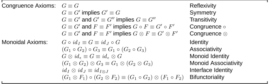
Table 3.1. Axioms
Congruence Axioms: G≡G Reflexivity
G≡G0impliesG0≡G Symmetry
G≡G0andG0≡G00impliesG≡G00 Transitivity
G≡G0andF ≡F0impliesG◦F ≡G0 ◦F0 Congruence◦
G≡G0andF ≡F0impliesG⊗F ≡G0 ⊗F0 Congruence⊗
Monoidal Axioms: G◦idI ≡G≡idJ ◦G Identity
(G1◦G2)◦G3≡G1◦(G2◦G3) Associativity
G⊗id≡G≡id⊗G Monoid Identity
(G1⊗G2)⊗G3≡G1⊗(G2⊗G3) Monoid Associativity
idI ⊗idJ ≡idI⊗J Interface Identity
(G1⊗F1)◦(G2⊗F2)≡(G1◦G2)⊗(F1◦F2) Bifunctoriality
3.1. Models
To evaluate formulae, we consider the terms freely generated from a set of constructorsΘby using the vertical composition (the partial composition ◦) and the horizontal composition (the partial tensor⊗). The order of binding precedence is◦,⊗. BiLog terms are defined asG, G0 ::= Ω|G ◦ G0 |G ⊗G0,
where Ωranges overΘ. We refer to these terms as bifunctorial terms, since the two operations must satisfy the bifunctoriality property of monoidal categories (the last rule in Table 3.1).
Terms are structures built on a monoid(M,⊗, )whose elements are dubbed interfaces and denoted byI, J. To model nominal resources, e.g. heaps or link graphs, the monoid may be partial. Intuitively, terms represent typed structures with a source and a target interface (G:I →J). Each constructorΩin
Θhas a fixed typetype(Ω) = I → J. For each interface I, we assume a distinguished constructidI :
I → I. The types of constructors, together with the obvious rules for composition and tensor [9, 18], determine the type of each term. Terms of type→ J are called ground. We consider only well typed terms.
Terms are defined up to a structural congruence≡(see Tab. 3.1) which subsumes the axioms of (par-tial) monoidal categories. All axioms are required to hold whenever both sides are well typed. Through-out the paper, when using =or≡we imply that both sides are defined; and when we need to remark that a bigraphical expressionEis well defined, we write(E)↓. The congruence will be refined to model specialised structures: place graphs, link graphs and bigraphs.
3.2. Formulae
BiLog internalises the bifunctorial terms in the style of the Ambient Logic [8]. Constructors appear in the logic as constant formulae, while tensor product and composition are expressed by connectives. Thus the logic presents two binary spatial operators. This contrasts with other spatial logics, that have a single operator: Spatial and Ambient Logics [3, 8], with the parallel compositionA|B, Separation Logic [23], with the separating conjunctionA∗B, and Context Tree Logic [5], with the applicationK(P). Both the operators inherit the monoidal structure and non-commutativity properties from the model.
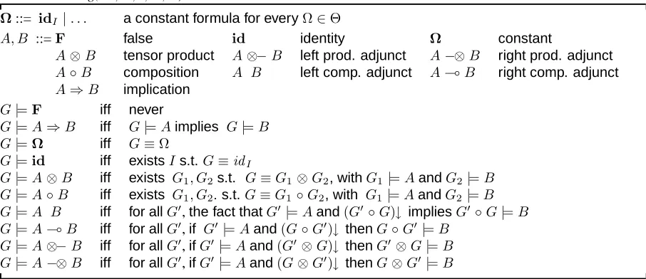
Table 3.2. BiLog(M,⊗, ,Θ,≡)
Ω::= idI |. . . a constant formula for everyΩ∈Θ
A, B ::=F false id identity Ω constant
A⊗B tensor product A⊗−B left prod. adjunct A−⊗B right prod. adjunct
A◦B composition A B left comp. adjunct A(B right comp. adjunct
A⇒B implication
G|=F iff never
G|=A⇒B iff G|=Aimplies G|=B
G|=Ω iff G≡Ω
G|=id iff existsIs.t.G≡idI
G|=A⊗B iff exists G1, G2s.t. G≡G1⊗G2, withG1|=AandG2|=B
G|=A◦B iff exists G1, G2.s.t.G≡G1◦G2, with G1|=AandG2|=B
G|=A B iff for allG0,the fact thatG0|=Aand(G0◦G)↓ impliesG0◦G|=B G|=A(B iff for allG0,if G0|=Aand(G◦G0)↓ thenG◦G0 |=B
G|=A⊗−B iff for allG0,ifG0|=Aand(G0⊗G)↓ thenG0⊗G|=B G|=A−⊗B iff for allG0,ifG0|=Aand(G⊗G0)↓ thenG⊗G0 |=B
semantics. The logic features a constantΩfor each constructΩand an identityidIfor each interfaceI. The satisfaction of logical constants is simply the congruence to the corresponding constructor. The horizontal decomposition formulaA ⊗ B is satisfied by a term that can be decomposed as the tensor product of two terms satisfyingAandB respectively. The degree of separation enforced by⊗between terms plays a fundamental role in the various instances of the logic, notably link graph and place graph. The vertical decomposition formula A ◦ B is satisfied by terms that can be the composition of terms satisfyingAandB. We shall see that in some cases both connectives correspond to well known spatial ones. We define the left and right adjuncts for composition and tensor to express extensional properties. The left adjunct A B expresses the property of a term to satisfy B whenever inserted in a context satisfying A. Similarly, the right adjunct A ( B expresses the property of a context to satisfy B
whenever filled with a term satisfyingA. A similar description holds for⊗−and−⊗, the adjoints of⊗. Clearly, these adjoints collapse whenever the tensor is commutative in the model.
3.3. Logical Equivalence
BiLog induces a logical equivalence =L on terms in the usual sense: we say that G1 =L G2 when
G1 |=Aif and only ifG2 |=Afor every formulaA. By induction on the structure of formulae, we can prove that the relation=Lrespects the congruence. We can prove that the logical equivalence coincides with the structural congruence, as every term admits a characteristic formula. This fact is fundamental to describe, query and reason about bigraphical data structures, as e.g. XML (cf. [11]). In other terms, BiLog is intensional in the sense of [25], namely it can observe internal structures, as opposed to the extensional logics used to observe the behaviour of dynamic system.
Theorem 3.1. (Logical equivalence is congruence)
Proof:
The forward direction is proved by defining the characteristic formula for terms, as every term can be expressed as a formula. The converse holds since=Lrespects the congruence. ut
The logical equivalence may be less discriminating when there are constructors not directly rep-resented by logical constants. The work in [12] show how the framework can be parameterised by a transparency predicate reflecting that not every term can be directly observed in the logic: some terms may be not visible to the logic or may be opaque without allowing inspection of their content. The particular characterisation of the logical equivalence given in Theorem 3.1 can be generalised to a con-gruence ‘up-to-transparency’: we can find an equivalence relation between trees that is ‘tuned’ by the transparency predicate – the more the predicate covers, the less the equivalence distinguishes [9, 18].
4.
Instances and encodings
In this section BiLog is instantiated to describe place graphs, link graphs and bigraphs. A spatial logic for bigraphs is a natural composition of a Place Graph Logic (for tree contexts) and a Link Graph Logic (for name linkings). Each instance admits an embedding of a well known spatial logic.
4.1. Place Graph Logic
Place graphs are essentially ordered lists of regions hosting unordered labelled trees with holes, namely contexts for trees. Tree labels correspond to the controlsK: 1→1belonging to a fixed signatureK. The monoid of interfaces is the monoid(ω,+,0)of finite ordinals, ranged over bym, n. Ordinals represent the number of holes and regions of place graphs. Place graph terms are generated from the set
Θ ={1 : 0→1, idn:n→n, join: 2→1, γm,n :m+n→n+m, K: 1→1forK∈ K}.
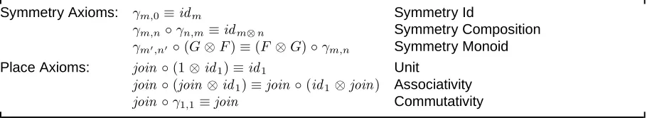
The only structured terms are the controlsK, representing regions containing a single node with a hole inside. All the other constructors are placings and represent trees m → n with no nodes: the place identityidnis neutral for composition; the constructor1represents a barren region;joinis a mapping of two regions into one;γm,nis a permutation that interchanges the firstmregions with the followingn. The structural congruence≡for place graph terms is refined in Tab. 4.1 by the usual axioms for symmetry of
γm,nand by the place axioms that essentially turn the operationjoin◦( ⊗ )in a commutative monoid with 1as neutral element. In particular, the places generated by composition and tensor product from
γm,nare permutations. A place graph is prime if it has typem→1, namely it has a single region. The Place Graph Logic PGL(K) isBiLog(ω,+,0,≡,K ∪ {1,join, γm,n}). Theorem 3.1 extends to PGL, thus the logic describes place graphs precisely. PGL resembles a propositional spatial tree logic as in [4], with the difference that PGL models contexts of trees and that the tensor product is not commutative, thus enabling the modelling of the order among regions. The logic can express a commutative separation by usingjoinand⊗, namely the parallel composition operator
A|B def
=join◦(id1◦A⊗id1◦B).
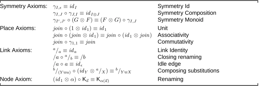
Table 4.1. Additional Axioms for Place Graphs Structural Congruence
Symmetry Axioms: γm,0≡idm Symmetry Id
γm,n◦γn,m≡idm⊗n Symmetry Composition
γm0,n0 ◦(G⊗F)≡(F ⊗G)◦γm,n Symmetry Monoid
Place Axioms: join◦(1⊗id1)≡id1 Unit
join◦(join⊗id1)≡join ◦(id1⊗join) Associativity
join◦γ1,1≡join Commutativity
Table 4.2. Propositional Spatial Tree Logic
T |=STLF iff never
T |=STL0 iff T ≡0
T |=STLA⇒B iff T |=STLA impliesT |=STL B
T |=STL a[A] iff there exists T0 s.t. T ≡a[T0] and T0|=STLA
T |=STL A@a iff a[T]|=STLA
T |=STL A|B iff there exists T0, T00 s.t. T ≡T0|T00 and T0|=STLA and T00|=STLB
T |=STL A . B iff for every T0: if T0|=STLA implies T |T0|=STLB
Encoding STL. Not surprisingly, prime ground place graphs are isomorphic to the unordered trees that model the static fragment of Ambient Logic. Here we show that BiLog, when restricted to prime ground place graphs, is equivalent to the propositional Spatial Tree Logic of [4] (STL in the following). The logic STL expresses properties of unordered labelled trees, ranged over by T, T0, T00 and constructed from the empty tree0, the labelled node containing a tree a[T], and the parallel composition of trees
T |T0. Labelsaare elements of a denumerable set. The obvious congruence≡on trees makes the set of trees with|and 0a commutative monoid. STL is a static fragment of the Ambient Logic [8] and it is characterised by the usual classical propositional connectives, the spatial connectives0,a[A],A |B, and their adjunctsA@a,A . B. The semantics of the logic is outlined in Tab. 4.2.
Table 4.3 encodes the tree model of STL into prime ground place graphs, and STL operators into PGL operators. We assume a bijective encoding between labels and controls, and we associate every labela
with a distinct controlK(a) of arity0. We assume two auxiliary notations: A ◦1 B =def A◦id1 ◦ B
which forces the composition to the interface1, andA 1 B = (def A ◦ id1) B, which guarantees terms
with target type 1. The monoidal properties of parallel composition are guaranteed by the axioms of join (symmetry and unit). The equations are self-explanatory once we remark that: (i) the parallel composition of STL is the structural commutative separation of PGL; (ii) tree labels can be represented by the corresponding controls of the place graph; (iii) location and composition adjuncts of STL are encoded by the left composition adjunct, as they add logically expressible contexts to the tree. This encoding is actually a bijection from trees to prime ground place graphs. In fact, there is an inverse encoding([ ])for prime ground place graphs in trees defined on the normal forms of [21] as we shall see. The theorem of discrete normal form in [21] implies that every ground place graph g : 0 → 1can be expressed, uniquely up to permutations, as g = joinn ◦ (M0 ⊗ . . . ⊗ Mn−1),where every Mj is a molecular prime ground place graph of the form M = K(a) ◦ g, with ar(K(a)) = 0. As an auxiliary notation, joinn is inductively defined asjoin0
def
= 1, andjoinn+1
def
Table 4.3. Encoding STL in PGL over prime ground place graphs
Trees into Prime Ground Place Graphs [[ 0 ]]def
=1 [[a[T] ]]def
=K(a)◦[[T]] [[T |T0]]def
=join ◦([[T]]⊗[[T0]])
STL formulae into PGL formulae [[0]]def
= 1 [[F]]def
=F [[a[A] ]]def
=K(a)◦1[[A]] [[A|B]]def= [[A]]|[[B]] [[A⇒B]]def
= [[A]]⇒[[B]] [[A@a]]=defK(a)1[[A]] [[A . B]]def= ([[A]]|id1)1[[B]]
The bifunctoriality property implies thatjoinn◦(M0 ⊗. . .⊗Mn−1)≡join ◦(M0 ⊗ · · · ⊗(join ◦
(Mn−2 ⊗Mn−1))).The inverse encoding([ ])is defined on the discrete normal form of prime ground
place graphs, and, along with[[ ]], it gives a bijection between trees and prime ground place graphs:
([join0])
def
= 0 ([K(a)◦q]) def
= a[ ([q]) ]
([joins◦(M0 ⊗. . .⊗Ms−1) ]) = ([def M0])|. . .|([Ms−1])
Theorem 4.1. (Encoding STL)
For each treeTand formulaAof STL:T |=STL Aif and only if[[T]]|= [[A]].
Proof:
Structural induction on STL formulae. The basic step involves the constantsFand0. ForFapply the definition. For 0: [[T]] |= [[0]] means[[T]] |= 1, that is[[T]] ≡ 1and soT ≡ ([ [[T]] ]) ≡ ([ 1 ]) def
= 0,
namelyT |=STL0. The inductive steps deal with connectives and modalities.
CaseA ⇒ B. To assume[[T]] |= [[A ⇒ B]]means[[T]] |= [[A]] ⇒ [[B]]; by definition this says that[[T]]|= [[A]]implies[[T]]|= [[B]]. By induction hypothesis, this is equivalent to say thatT |=STLA
impliesT |=STL B, namelyT |=STLA⇒B.
Casea[A]. To Assume[[T]]|= [[a[A] ]]means[[T]]|=K(a)◦1 ([[A]]). Then there existG: 1→1
and g : 0 → 1such that [[T]] ≡ G ◦ g and G |= K(a)and g |= [[A]], that is[[T]] ≡ K(a) ◦ g with
g |= [[A]]. Then T ≡ ([K(a) ◦ g]) def
= a[([g])] with g |= [[A]], as the encoding is bijective. Since
g: 0→1, the induction says that([g])|=A. HenceT |=STLa[A].
CaseA@a. To assume[[T]] |= [[A@a]] means[[T]] |=K(a) 1 A, which says that if(G ◦ [[T]])↓
thenG◦[[T]]|= [[A]], for everyGsuch thatG|=K(a). By definition, this isK(a)◦[[T]]|= [[A]], then
[[a[T] ]]|= [[A]]. By induction, this isa[T]|=STL A. HenceT |=STLA@aby definition.
CaseA|B. To assume[[T]] |= [[A |B]]means[[T]]|= [[A]]|[[B]]. This is equivalent to say that
[[T]] |=join ◦ (id1◦[[A]]⊗id1 ◦[[B]]), namely there existg1, g2 : 0 → 1such that[[T]] ≡ join ◦
(g1 ⊗g2)andg1 |= [[A]]andg2 |= [[B]]. As the encoding is bijective this means thatT ≡([g1])|([g2]), and the induction hypothesis says that([g1])|=Aand([g2])|=B. By definition this isT |=STL A|B.
Case A . B. To assume [[T]] |= [[A . B]] means [[T]] |= join([[A]]⊗id1)) 1 [[B]] – i.e.,
for every G : 1 → 1 if G |= join([[A]]⊗id1) then G ◦ [[T]] |= [[B]]. Now, G : 1 → 1 and G|=join([[A]]⊗id1)means that there existsg : 0→ 1such thatg |= [[A]]andG≡join(g⊗id1).
Hence for every g : 0 → 1 such that g |= [[A]] it holds join(g⊗id1) ◦ [[T]] |= [[B]], that is
join(g⊗[[T]]) |= [[B]] by bifunctoriality. As[[ ]] is bijective, for everyT0 such that [[T0]] |= [[A]]
it holds join([[T0]]⊗[[T]]) |= [[B]] – i.e., [[T0 | T]] |= [[B]]. By induction, for every T0 such that
T0 |=
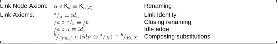
Table 4.4. Additional Axioms for Link Graph Structural Congruence
Link Node Axiom: α◦K~a ≡Kα(~a) Renaming
Link Axioms: a/
a≡ida Link Identity
/a◦a/
b≡/b Closing renaming
/a◦a≡id Idle edge
b/
(Y]a)◦(idY ⊗a/X)≡b/Y]X Composing substitutions
Differently from STL, PGL can also describe structures with several holes and regions. In [11] we show that PGL can describe contexts of tree-shaped semistructured data. Consider, for instance, a function taking two trees and returning the tree obtained by merging their roots. Such a function is represented by the termjoin, which solely satisfies the formulajoin. Similarly, a function that takes a tree and encapsulates it inside a node labelled byK, is represented by the term Kand captured by the formulaK. Moreover, the formulajoin ◦ (K ⊗ (T ◦ id1))expresses all contexts of form 2 → 1that
place their first argument inside the nodeKand their second one as a sibling of such node.
4.2. Link Graph Logic (LGL)
Fixed a denumerable set of namesΛ, we consider the monoid(Pfin(Λ),],∅), wherePfin( )is the finite
powerset operator and]is the disjoint union of subsets. Link graphs are the structures arising from such a monoid. They can describe nominal resources, which are common in many areas: object identifiers, location names in memory structures, channel names, and ID attributes in XML documents. Due to the disjoint union, names cannot be shared implicitly; anyway, they can be referred to or linked explicitly (e.g. as object references, location pointers, fusion in fusion calculi, and IDREF in XML files). Link graphs describe connections between resources performed by means of names, that are references.
Wiring terms are a structured way to map a set of inner namesXinto a set of outer namesY. They are generated by the constructors: /a:{a} → ∅anda/X :X →a. The closure/ahides the inner name
ain the outer face. The substitutiona/X associates all the names in the setXto the namea. We denote wirings byω, substitutions byσ, τ, and bijective substitutions, dubbed renamings, byα, β. Substitution can be specialised ina def
= a/∅, which introduces the namea, ina← b=def a/{b}, which renamesbtoa,
and ina⇔b=def a/{a,b}, which linksaandbtoa.
Another class of constructors for link graphs are the controls Kin the signature K. They represent nodes associated to names, and they have fixed arities to determine the number of ports – i.e., the number of the outer names associated to the control. Arity is given by the arity functionar :K →N. Link graphs
are generated from wirings and the constructorsK~a:∅ →~awith~a=a1, . . . , ak,K∈ Kandk=ar(K). The controlK~arepresents a resource of kindKwith named ports~a. Any ports may be connected to other node ports via wiring compositions. The structural congruence≡is refined as outlined in Tab. 4.4 with the obvious axioms for links, which modelα-conversion and extrusion of closed names. In this case, the horizontal decomposition inherits the commutativity property from the monoidal tensor product.
resources with local (hidden or private) names, and in this sense it is a generalisation of Spatial Graph Logic [6]. To see this it is sufficient to consider the edges as resources.
The formulaA ⊗ B describes a decomposition into two separate link graphs, which share neither resources, nor names, nor connections, and which satisfy AandB respectively. Since it is defined only on link graphs with disjoint inner/outer sets of names, the tensor product is a kind a spatial/separation operator, in the sense that it separates the model into two distinct parts that cannot share names.
If we want a nameato be shared between separated resources, we need to make the sharing explicit, and we can do that only through the link operation. We therefore need a way to first separate the names occurring in two wirings in order to apply the tensor, and then link them back together, as shown next.
As a shorthand, ifW : X → Y and W0 : X0 → Y0 with Y ⊂ X0, we write[W0]W for(W0 ⊗
idX0\Y)◦W and if~a=a1, . . . , anand~b=b1, . . . , bn, we write~a←~bfora1 ←b1 ⊗. . .⊗an←bn, similarly for~a⇔~b. From the tensor product it is possible to derive a product with sharing on~a. Given
G:X→Y andG0:X0 →Y0withX∩X0 =∅, we choose a list~b(with the same length as~a) of fresh names. The composition with sharing on~ais
G⊗~aG0 def
= [~a⇔~b]([~b←~a]G⊗G0).
In this case, the tensor product is well defined since all the common names~ainGare renamed to fresh names, while the sharing is re-established afterwards by linking the names in~awith the names in~b.
By extending this sharing to all names we can define the parallel composition G | G0 as a total operation. However, such an operator does not behave ‘well’ with respect to the composition, as shown in [21]. In addition, a direct inclusion of a corresponding connective in the logic would impact the satisfaction relation by expanding the finite horizontal decompositions to the boundless possible name-sharing decompositions. This is due to the fact that the set of names shared by a parallel composition is not known in advance, and therefore parallel composition can only be defined by using an existential quantification over the entire set of shared names.
Names can be internalised and effectively made private to a bigraph by the closure operator/a. In fact, the effect of the composition with /a is to add a new edge with no public name, and therefore to make a disappear from the outerface and be completely hidden to the outside. Separation is still expressed by the tensor connective. This connective not only separates places, but also ensures that no edge, whether visible or hidden, crosses the separating line.
As a matter of fact, without name quantification it is not possible to build formulae that explore a link, since the closure has the effect of hiding names. For this task, we employ the name variablesx1, ..., xn and the fresh name quantificationNin the style of Nominal Logic [24]. The semantics is defined as
G|=Nx1. . . xn. Aiff there exista1. . . an∈/ fn(G)∪fn(A)such thatG|=A{x1...xn/
a1...an},
whereA{x1...xn/
a1...an}is the usual variable substitution.
By fresh name quantification we define a notion of~a-linked name quantification for fresh names, whose purpose is to identify names linked to~a, as
~aL~x. A def
=N~x.((~a⇔~x)⊗id)◦A.
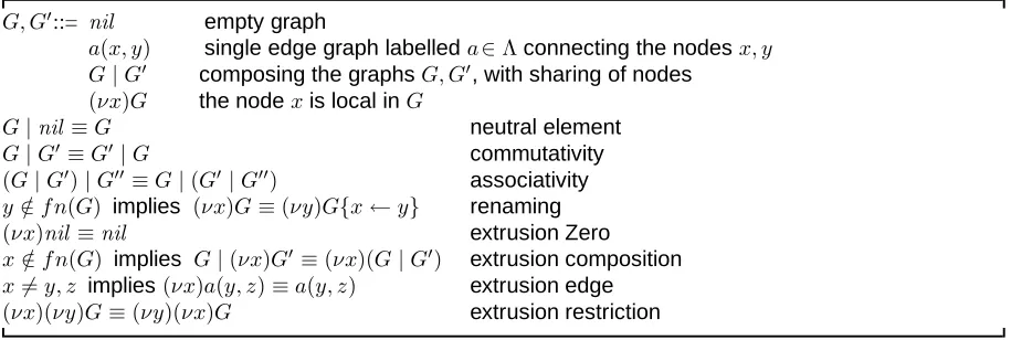
Table 4.5. Spatial graph Terms (with local names) and congruence
G, G0::= nil empty graph
a(x, y) single edge graph labelleda∈Λconnecting the nodesx, y
G|G0 composing the graphsG, G0, with sharing of nodes
(νx)G the nodexis local inG
G|nil ≡G neutral element
G|G0≡G0|G commutativity
(G|G0)|G00≡G|(G0 |G00) associativity
y /∈f n(G) implies (νx)G≡(νy)G{x←y} renaming
(νx)nil ≡nil extrusion Zero
x /∈f n(G) implies G|(νx)G0 ≡(νx)(G|G0) extrusion composition x6=y, z implies(νx)a(y, z)≡a(y, z) extrusion edge
(νx)(νy)G≡(νy)(νx)G extrusion restriction
separation-up-to as the decomposition in two terms that are separated apart from the link on the specific names in~a, which crosses the separation line:
A⊗~aB def
=~aL~x.(((~x←~a)⊗id)◦A)⊗B.
The idea expressed by this formula is that the shared names~aare renamed in fresh names~x, so that the product can be performed and finally~xis linked to~ato actually have the sharing. It is straightforward to prove that the two definitions are consistent.
Lemma 4.1. (Separation-up-to)
Ifg|=A⊗X~ B withg:→ X, andX~ is the vector of the elements inX, then there existg1 :→X
andg2 :→Xsuch thatg≡g1 ⊗X~ g2withg1 |=Aandg2|=B.
Proof:
Apply the definitions and observe that the identities forcing idmust be id, as the outer face of g is
X. ut
The corresponding parallel composition operator is not directly definable by using the separation-up-to. In fact, in arbitrary decompositions the shared names are not all known a priori, hence we would not know the vectorX~ in the operator sharing/separation operator ⊗X~. However, next section shows that a careful encoding is possible for the parallel composition of spatial logics with nominal resources.
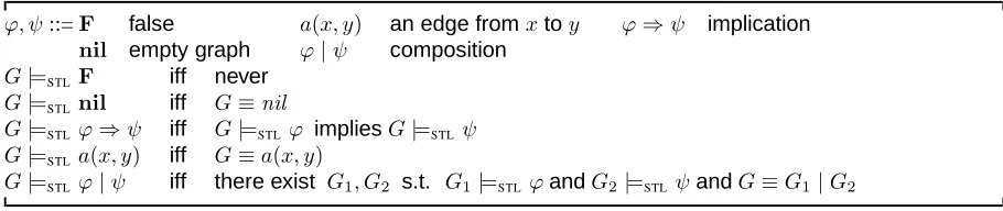
Encoding SGL. Here we show that LGL can be seen as a contextual (multi-edge) version of Spatial Graph Logic (SGL) [6], which expresses properties of directed graphsGwith labelled edges. The syntax of graphs outlined in Tab. 4.5. The notationa(x, y)represents an edge from the nodextoyand labelled by a. The graphs G are built from the empty graph nil and the edge a(x, y) by using the parallel compositionG1|G2 and the binding for local names of nodes(νx)G.
Table 4.6. Propositional Spatial Graph Logic (SGL)
ϕ, ψ::=F false a(x, y) an edge fromxtoy ϕ⇒ψ implication
nil empty graph ϕ|ψ composition
G|=STLF iff never
G|=STLnil iff G≡nil
G|=STLϕ⇒ψ iff G|=STLϕ impliesG|=STLψ
G|=STLa(x, y) iff G≡a(x, y)
G|=STLϕ|ψ iff there exist G1, G2 s.t. G1|=STL ϕandG2|=STLψandG≡G1|G2
Table 4.7. Encoding Propositional SGL in LGL over ground link graphs
Spatial Graphs into Two-ported Ground Link Graphs
[[nil]]X def=X [[ (νx)G]]X def= ((/x⊗idX\{x})◦[[G]]{x}∪X))⊗({x} ∩X)
[[a(x, y) ]]X=defK(a)x,y⊗X\ {x, y} [[G|G0]]X def= [[G]]X⊗X~ [[G0]]X
SGL formulae into LGL formulae
[[nil]]X def=X [[a(x, y) ]]X def=K(a)x,y ⊗(X\ {x, y}) [[ϕ|ψ]]X= [[def ϕ]]X ⊗X~ [[ψ]]X
[[F]]X def=F [[ϕ⇒ψ]]X def= [[ϕ]]X ⇒[[ψ]]X
language for graphs. In addition, the logic is integrated with transducers to allow graph transformations. The applications of SGL include description and manipulation of semistructured data. Table 4.6 depicts the syntax and the semantics of the fragment we consider.
For the encoding, we consider a signature K with controls of arity 2, and we assume a bijective function associating every labelato a distinct controlK(a). The ports represent the starting and arrival node of the associated edge. The resulting link graphs are interpreted as contextual graphs with labelled edges, whereas the resulting class of ground link graphs is isomorphic to the graph model of SGL.
Table 4.7 encodes the graphs that model SGL into ground link graphs and SGL formulae into LGL formulae. The encoding is parametric on a finite setX of names which contains the free names of the graph. As we force the outer face of the graphs to be a fixed setX, the encoding of parallel composition is simply a separation-up-to the elements X~ ofX. Local names are encoded into name closures. The Connected Normal Form of [21] helps in proving that ground link graphs featuring controls with exactly two ports are isomorphic to spatial graph models.
Lemma 4.2. (Isomorphism for spatial graphs)
There is a mapping ([ ])from two-ported ground bigraphs to spatial graphs, such that for every set X
of names: (i) the mapping([ ])is inverse to[[ ]]X; (ii) for every ground link graphg with outer faceX featuring a countable set of controlsK, all with arity2, it holdsf n(([g])) = Xand[[ ([g]) ]]X ≡g; and (iii) for every spatial graphGwithf n(G) =Xit holds[[G]]X :→Xand([ [[G]]X])≡G.
Proof:
[image:13.595.76.528.280.370.2]Kx,y(a)◦1. The inverse encoding is based on this normal form:
([ (/Z|idh1,Xi)◦(X|M0 |. . .|Mk−1) ])= (def νZ) (nil |([M0])|. . .|([Mk−1]))
([Kx,y(a)◦1 ])=def a(x, y)
The encodings[[ ]]and([ ])provide a bijection between graphs with free namesXand ground link graphs with outer faceXand controls of arity two. ut
Theorem 4.2. (Encoding SGL)
For every graph G, every finite set X that contains fn(G), and every formula ϕ of the propositional fragment of SGL:G|=SGLϕif and only if[[G]]X |= [[ϕ]]X.
Proof:
By induction on formulae of SGL. The basic steps deal with the constantsF,nilanda(x, y).The case
Ffollows by definition. For the case nil, [[G]]X |= [[nil]]X means[[G]]X |= X, that by definition is
[[G]]X ≡Xand soG≡([ [[G]]X ])≡([X])=defnil, namelyG|=SGLnil. For the casea(x, y), to assume
[[G]]X |= [[a(x, y) ]]X means [[G]]X |= K(a)x,y ⊗ X \ {x, y}. SoG ≡ ([ [[G]]X]) ≡ ([K(a)x,y ⊗
X\ {x, y}])≡a(x, y), that isG|=SGLa(x, y). The inductive steps deal with connectives.
Caseϕ ⇒ ψ. [[G]]X |= [[ϕ ⇒ ψ]]X means[[G]]X |= [[ϕ]]X ⇒ [[ψ]]X that is: [[G]]X |= [[ϕ]]X implies[[G]]X |= [[ψ]]X. By induction, this means thatG |=SGL ϕimpliesG |=SGL ψ – i.e.,G |=SGL
ϕ⇒ψ.
Caseϕ|ψ. [[G]]X |= [[ϕ|ψ]]X means[[G]]X |= [[ϕ]]X ⊗ ~ X [[ψ]]
X. By Lemma 4.1 there existsg1,
g2such that[[G]]X ≡g1 ⊗ ~
X g2and g1 |= [[ϕ]]
X andg2 |= [[ψ]]X. LetG1 = ([g1])andG2 = ([g2]), then[[G1]]X ≡ g1 and[[G2]]X ≡ g2. Hence[[G1]]X |= [[ϕ]]X and [[G2]]X |= [[ψ]]X. By induction:
G1 |=SGL ϕandG2 |=SGL ψ. Now,[[G1 |G2]]X ≡[[G1]]X ⊗X~ [[G2]]X ≡g1 ⊗X~ g2 ≡ [[G]]X, thus
G|=SGLϕ|ψ. ut
LGL enables the encoding of Separation Logic for heaps: names used as identifiers of location are forcibly separated by tensor product, while names used for pointers are shared/linked. However we do not encode it explicitly since in§4.3 we will encode a more general logic: the Context Tree Logic [5].
4.3. Pure Bigraph Logic
By combining link graphs and place graphs we generate all the (abstract pure) bigraphs of [17]. In this case the underlying monoid is the product of link and place interfaces, namely(ω× Pfin(Λ),⊗, )where
hm, Xi ⊗ hn, Xi def
= hm+n, X]Yiand def
=h0,∅i. As a short notation, we useXforh0, Xiandn
forhn,∅i.
A set of constructors for bigraphical terms is obtained as the union of place and link graph con-structors. Only controls are subsumed by the new discrete ion constructors, which are denoted by
K~a : 1 → h1,~ai and represent prime bigraphs containing a single node with ports named~a and an hole inside. Bigraphical terms are thus defined in relation to a control signatureKand a set of namesΛ, as detailed in [21].
Table 4.8. Additional axioms for Bigraph Structural Congruence
Symmetry Axioms: γI,≡idI Symmetry Id
γI,J ◦γJ,I ≡idI⊗J Symmetry Composition
γI0,J0 ◦(G⊗F)≡(F ⊗G)◦γI,J Symmetry Monoid
Place Axioms: join ◦(1⊗id1)≡id1 Unit
join ◦(join ⊗id1)≡join◦(id1⊗join) Associativity
join ◦γ1,1≡join Commutativity
Link Axioms: a/
a≡ida Link Identity
/a◦a/
b≡/b Closing renaming
/a◦a≡id Idle edge
b/
(Y]a)◦(idY ⊗a/X)≡b/Y]X Composing substitutions
Node Axiom: (id1⊗α)◦K~a ≡Kα(~a) Renaming
PGL excels at expressing properties of unnamed resources, that are resources accessible only by following the structure of the term. On the other hand, LGL characterises names and their links to resources, but it has no notion of locality. A combination of this two logics is useful to model nominal spatial structures, either private or public.
BiLog promises to be a good (contextual) spatial logic for (semi-structured) resources with nominal links, thanks to bigraphs’ orthogonal treatment of locality and connectivity. To testify this, next section shows how the Context Logic for Trees (CTL) [5] can be encoded into bigraphs.
Encoding CTL. In [5] the authors propose a spatial context logic to describe programs manipulating a tree structured memory. The model of the logic is the set of unordered labelled trees T, T0, T00 and linear contexts C, C0, C00 which are trees with a unique hole. Every node has a name, so to identify memory locations. The logic is dubbed Context Tree Logic, CTL in the following. Given a denumerable set of labels and a denumerable set of identifiers, trees and contexts are defined in Tab. 4.9:arepresents a label and x an identifier. The insertion of a tree T in a context C, denoted by C(T), is defined in the standard way by filling the unique hole of C withT. A well formed tree or context is one where the node identifiers are unique. The model of the logic is composed by well formed trees and contexts. Composition, node formation and tree insertion are partial as they are restricted to well-formed trees. The structural congruence between trees and contexts is the smallest congruence that makes the parallel operator to be commutative, associative and with the empty tree as neutral element.
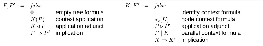
The logic exhibits two kinds of formulae: P, describing trees, andK, describing tree contexts. It has two spatial constants, the empty tree forP and the hole forK, and four spatial operators: the node formation ax[K], the application K(P), and its two adjunctsK . P and P1 / P2. The formulaax[K] describes a context with a single root labelled byaand identified byx, whose content satisfiesK. The formulaK . P represents a tree that satisfiesP whenever inserted in a context satisfying K. Dually,
P1/ P2 represents contexts that composed with a tree satisfyingP1 produce a tree satisfyingP2. The complete syntax of the logic is outlined in Tab. 4.10, the semantics in Tab. 4.11.
Table 4.9. Trees with pointers and Tree Contexts
T, T0 ::= 0 empty tree
ax[T] a tree labelledawith identifierxand subtreeT T |T0 partial parallel composition
C ::= − an hole (the identity context)
ax[C] a tree context labelledawith identifierxand subtreeC
T |C context right parallel composition
C|T context left parallel composition
T |0≡T neutral element
T |T0≡T0|T commutativity
(T |T0)|T00≡T |(T0|T00) associativity
(T |T0)↓ if and only if identifiers ofT andT0are disjoint
similarly for contexts
Table 4.10. Context Tree Logic (CTL)
P, P0::= false K, K0::= false
0 empty tree formula − identity context formula
K(P) context application ax[K] node context formula
K / P application adjunct P . P0 application adjunct
P ⇒P0 implication P |K parallel context formula
K⇒K0 implication
location in the memory. This property is obtained with bigraphs by encoding the identifiers as names and the composition as tensor product. This structure is then encoded in BiLog by lifting the application between contexts and trees to a particular kind of composition.
The tensor product on bigraphs is both a spatial separation, like in the models for STL, and a partially-defined separation on names, like pointer composition for Separation Logic. Since we deal with both names and places, we define a formulaidhm,ito represent identities on places by constraining the place part of the interface to be fixed and leaving the name part to be free: idhm,i =def idm ⊗ (id∧ ¬(T ⊗
id1 ⊗ T)). The semantics says thatG |=idhm,−iif and only if there exits a set of namesXsuch that G ≡ idm ⊗ idX. By using such an identity formula we define the corresponding typed composition
A ◦hm,i B =def A ◦ idhm,i ◦ B and the typed adjuncts: A hm,i B = (def idhm,i ◦ A) B andA (hm,i B def
= (A◦idhm,i) B.
We then encode the operator for the parallel composition by the separation operator∗defined as both a term constructor and a logical connective: G∗G0 def
= [join](G⊗G0)on prime bigraphs, and
A∗B def
= (join⊗idh0,i)◦(idh1,i ◦A⊗idh1,i ◦B)
on formulae. The operator ∗ enables the encoding of trees and contexts into bigraphs. Finally, we consider a signature with controls of arity1 and we assume a bijective function from tags to controls:
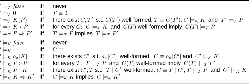
[image:16.595.67.521.336.416.2]Table 4.11. Semantics for CTL
T |=T false iff never
T |=T 0 iff T ≡0
T |=T K(P) iff there existC, T0 s.t.C(T0)well-formed,T ≡C(T0), C|=KK and T0|=T P T |=T K / P iff for everyC: C|=KK and C(T)well-formed imply C(T)|=T P
T |=T P ⇒P0 iff T |=T Pimplies T |=T P0 C|=K false iff never
C|=K − iff C≡ −
C|=K ax[K] iff there existsC0 s.t.ax[C0] well-formed, C≡ax[C0]and C0 |=KK C|=K P . P0 iff for everyT: T|=T P and C(T)well-formed imply C(T)|=T P0
C|=K P|K iff there existC0, T s.t. T|C0 well-formed,C≡T |C0,T |=T P and C0|=K K C|=K K⇒K0 iff C|=KKimplies C|=KK0
Paper [21] shows that the normal form, up to permutations, for ground prime discrete bigraphs is
g= (joink⊗idX)◦(M1 ⊗. . .⊗Mk),whereMi are called discrete ground molecules and are of the formM = (K(a)x ⊗idY)g.Thanks to this result, we can define the reverse encoding([ ])of[[ ]], from ground prime discrete bigraphs to trees, just by considering such a normal form:
([join0])
def
= 0
([ (K(a)x ⊗idY)◦g]) =def ax[ ([g]) ]
([ (joink⊗idY)◦(M1 ⊗. . .⊗Mk) ]) = ([def M1])∗. . .∗([Mk])
Moreover, the encodings of linear contexts are the unary discrete bigraphs G – i.e., bigraphs with open links and type h1, Xi → h1, Yi. Again, [21] says that the normal form, up to permutations, for unary discrete bigraphs is: G= (joink ⊗ idY) ◦ (R ⊗ M1 ⊗ . . . ⊗Mk−1),whereMi are discrete ground molecules andRcan be eitherid1 or(K~a ⊗idY)◦ Q. Again, we can define the reverse encoding([ ])
of[[ ]], from unary discrete bigraphs to linear contexts, just by considering such a normal form:
([id1]) =def −
([ (K(a)x⊗idY)◦Q]) =def ax[([Q])]
([ (joink ⊗idY)◦(R⊗M1 ⊗. . .⊗Mk−1) ]) = ([def R])|([M1])|. . .|([Mk−1])
As the model is specialised to context trees, so BiLog is specialised to the Context Tree Logic. The encoding of the logic is in Tab. 4.12, and the proof of soundness mimes Theorems 4.1 and 4.2.
Theorem 4.3. (Encoding Context Tree Logic)
For each tree T and formulaP of CTL,T |=T P if and only if[[T]] |= [[P]]P. Moreover, for each contextCand formulaKof CTL,C|=KKif and only if[[C]]C |= [[K]]K.
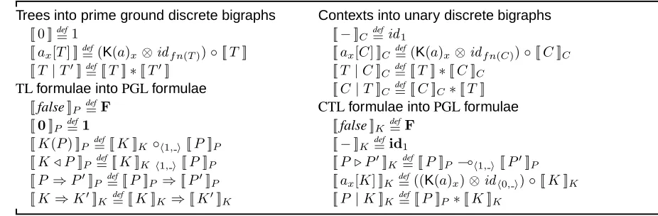
Table 4.12. Encoding CTL in BiLog over prime discrete ground bigraphs
Trees into prime ground discrete bigraphs Contexts into unary discrete bigraphs
[[ 0 ]]def
= 1 [[−]]Cdef=id1
[[ax[T] ]]= (def K(a)x⊗idf n(T))◦[[T]] [[ax[C] ]]C def= (K(a)x⊗idf n(C))◦[[C]]C
[[T |T0]]def
= [[T]]∗[[T0]] [[T |C]]C= [[def T]]∗[[C]]C
TLformulae intoPGLformulae [[C|T]]C= [[def C]]C∗[[T]]
[[false]]P def=F CTLformulae intoPGLformulae
[[0]]P =def1 [[false]]K def=F
[[K(P) ]]P def= [[K]]K ◦h1,i[[P]]P [[−]]K=defid1
[[K / P]]P def= [[K]]K h1,i[[P]]P [[P . P0]]K= [[def P]]P (h1,i[[P0]]P
[[P ⇒P0]]
P = [[def P]]P ⇒[[P0]]P [[ax[K] ]]K def= ((K(a)x)⊗idh0,i)◦[[K]]K
[[K⇒K0]]
K = [[def K]]K ⇒[[K0]]K [[P|K]]K= [[def P]]P∗[[K]]K
5.
BiLog and separation
The notion of separation in BiLog is not fixed a priori, but it relies on the projection of the tensor product to the logical level. The operators of the model, along with their logical projections, inherit the characteristics and the behaviour from the underlying resource monoid. This fact is fundamental to express the notions of separation/composition of other logics. When the resource monoid is partial, then the tensor product of terms is partial as well, and thus its logical projection describes only well-defined structures. Take for instance the heap memory addresses formalised by sets of names and consider their disjoint union. In this case we find the operator ∗of Separation Logic, which says nothing about the structures that do not have disjoint set of names, because they are not well-defined heaps. When the resource monoid is commutative, then also the tensor product is commutative, its logical projection is commutative and its two adjuncts collapse.
When we consider ordinals (as for place graphs) the tensor product is total, as it corresponds to placing two structures one next to the other, and the separation is total and purely structural, like for the Spatial Tree Logic. Notice that a commutative monoid combined with bifunctoriality has a peculiar behaviour with respect to composition: for instance, given the controlsK1 and K2, commutativity and
bifunctoriality would say that (K1 ◦ K1) ⊗ (K2 ◦ K2) and (K1 ◦ K2) ⊗ (K2 ◦ K1) are congruent
as both are congruent to (K1 ⊗ K2) ◦ (K1 ⊗ K2). Thus commutativity cannot hold when controls
are intended as places. While the parallel composition for ground structures is commutative, the tensor product for placing contexts is not commutative. Consequently, the left and right tensor adjuncts have different semantics in place graphs.
When ordinals and names are combined, the logic inherits their orthogonality. The resulting monoid can be seen as the product of two monoids, the one for ordinals (e.g. place graph) and the other for names (e.g. link graph). The constructive character of this approach says that, independently of the complexity of the underlying algebra and the resource model, we can split the model into ‘smaller’ parts and combine the corresponding logics to obtain a spatial logic for the desired model in a compositional way.
heaps, and thus to have a natural encoding of Separation Logic. The separation induced by the tensor product would be more strict than heap separation, as it forces also values to be separated. The heap composition can be achieved by forcing the sharing of pointers and values and by preserving the sepa-ration of addresses. The derived logical operators would behave as the tensor product on the names in the first sort (the addresses) and as a (kind of) parallel composition for the names in the second sort (the values/pointers). We do not necessarily need closure or restriction to model heaps. Open link graphs are sufficient. Similarly, open discrete bigraphs are sufficient for trees with pointers.
6.
Conclusions and related work
This paper moves a first step towards describing global resources by focusing on bigraphs. Our final objective is to design a general dynamic logic able to cope uniformly with all the models bigraphs have been proved useful for, as of today these include Petri-nets [20], CCS [22], π-calculus [17], ambient calculus [16], and context-aware systems [1]. Here we introduce the static fragment of BiLog, a logic founded on bigraphs, whose formulae describe arrows in monoidal categories.
BiLog may at first appear complex and ‘over-provided’ of connectives. On the contrary, the backbone of the logic is relatively simple, consisting of two connectives regulated by elementary monoidal and interchange laws. This structure gives rise to many – occasionally complex – derived connectives. This is a fundamental expressiveness property that does not put us off, as BiLog is meant to be a comprehensive meta-level framework in which several different logics can be isolated, understood and compared.
In particular, here show how the ‘separation’ plays in various fragments of the logic. For instance, in the case of Place Graph Logic, where models are bigraphs without names, the separation is purely structural and coincides with the notion of parallel composition in Spatial Tree Logic. Dually, as the models for Link Graph Logic are bigraphs with no location, the separation in LGL is disjointness of nominal resources. Finally, for Bigraph Logic, where nodes of the model are associated with names, the separation is not only structural, but also nominal, since the constraints on composition force port identifiers to be disjoint. In this sense, it can be seen as the separation in memory structures with pointers, like Separation Logic’s heap structures [23], and trees with either pointers [5] or hidden names [7].
The work in [10] proves that unrestricted sharing combined with name restriction makes the logic undecidable. The sharing/separation operator provided here hints that the real cause of undecidability is the quantification on the set of names and suggests that the decidability result of [4] can be extended to logics with explicit sharing and name revelation. We leave the this issue for future work.
In§3 we observed that the induced logical equivalence coincides with the structural congruence of terms. This property is fundamental to describe, query and reason about bigraphical data structures. For a more detailed discussion we refer to [11], where we sketch the application of BiLog to XML data.
To be as free as possible in choosing the level of intensionality and to ‘tune’ the power of the logical equivalence, the general definition for BiLog (c.f. [12]) is parameterised on a transparency predicate, whose role is to identify the terms allowing inspection of their content, transparent terms, and the ones that do not, opaque terms. Theorem 3.1 says that the logical equivalence is the structural congruence if every term is transparent, but [9, 18] show how BiLog becomes less discriminating with opaque terms.
is ‘intensional’ in the sense of [25], as it can observe internal structures. In the case of the bigraphical system describing CCS [22], BiLog can be so intensional that its static fragment directly expresses a temporal modality. A transparency predicate specifies which structures can be directly observed by the logic, while a temporal modality, along with the spatial connectives, allows to deduce the structure by observing the behaviour. It would be interesting to isolate some fragments of the logic and investigate how the transparency predicate influences their expressivity and intensionality, as done in [15]. Finally the papers [13, 14] suggest applications and extensions for BiLog.
References
[1] Birkedal, L., Debois, S., Elsborg, E., Hildebrandt, T., Niss, H.: Bigraphical Models of Context-aware Sys-tems, FOSSACS, 2006.
[2] Birkedal, L., Debois, S., Hildebrandt, T.: Sortings for Reactive Systems, CONCUR, 2006.
[3] Caires, L., Cardelli, L.: A Spatial Logic for Concurrency (Part I), TACS, 2001.
[4] Calcagno, C., Cardelli, L., Gordon, A.: Deciding Validity in a Spatial Logic for Trees, TLDI, 2003.
[5] Calcagno, C., Gardner, P., Zarfaty, U.: A Context Logic for Tree Update, POPL, 2005.
[6] Cardelli, L., Gardner, P., Ghelli, G.: A Spatial logic for querying graphs, ICALP, 2002.
[7] Cardelli, L., Gardner, P., Ghelli, G.: Manipulating Trees with Hidden Labels, FOSSACS, 2003.
[8] Cardelli, L., Gordon, A.: Ambient Logic, Mathematical Structures in Computer Science, To appear.
[9] Conforti, G.: Spatial Logics for Semistructured Resources, PhD Thesis, Univ. of Pisa, 2005.
[10] Conforti, G., Ghelli, G.: Decidability of Freshness, Undecidability of Revelation, FOSSACS, 2004.
[11] Conforti, G., Macedonio, D., Sassone, V.: Bigraphical Logics for XML, SEBD, 2005.
[12] Conforti, G., Macedonio, D., Sassone, V.: Spatial Logics for Bigraphs, ICALP, 2005.
[13] Damgaard, T., Birkedal, L.: Axiomatizing binding bigraphs, Nordic Journal of Computing, 13(1), 2006.
[14] Grohmann, D., Miculan, M.: Directed Bigraphs, MFPS, 2007.
[15] Hirschkoff, D.: An Extensional Spatial Logic for Mobile Processes, CONCUR, 2004.
[16] Jensen, O.: Forthcoming PhD Thesis, Aalborg Univ.
[17] Jensen, O., Milner, R.: Bigraphs and mobile processes (revised), Tech. rep., Univ. of Cambridge, 2004.
[18] Macedonio, D.: Logics for Distributed Resources, PhD Thesis, Univ. Ca’ Foscari of Venice, 2006.
[19] Milner, R.: Bigraphical Reactive Systems, CONCUR, 2001.
[20] Milner, R.: Bigraphs for Petri nets, Lectures on Concurrency and Petri Nets: Advances in Petri Nets, 2004.
[21] Milner, R.: Axioms for bigraphical structure, Mathematical Structures in Computer Science, 15(6), 2005.
[22] Milner, R.: Pure bigraphs: Structure and dynamics, Information and Computation, 204(1), 2006.
[23] O’Hearn, P., Reynolds, J., Yang, H.: Local Reasoning about Programs that Alter Data Structures, CSL, 2001.
[24] Pitts, A.: Nominal Logic: a First Order Theory of Names and Binding, TACS, 2001.