Microflow valve control system design

http://pii.sagepub.com/

Control Engineering

Engineers, Part I: Journal of Systems and

http://pii.sagepub.com/content/225/3/431

The online version of this article can be found at:

DOI: 10.1177/2041304110394519

2011 225: 431

Proceedings of the Institution of Mechanical Engineers, Part I: Journal of Systems and Control Engineering

R Zante and X T Yan

Microflow valve control system design

Published by:

http://www.sagepublications.com

On behalf of:

Institution of Mechanical Engineers

can be found at:

Engineering

Proceedings of the Institution of Mechanical Engineers, Part I: Journal of Systems and Control

Additional services and information for

http://pii.sagepub.com/cgi/alerts

Email Alerts:

http://pii.sagepub.com/subscriptions

Subscriptions:

http://www.sagepub.com/journalsReprints.nav

Reprints:

http://www.sagepub.com/journalsPermissions.nav

Permissions:

http://pii.sagepub.com/content/225/3/431.refs.html

Citations:

What is This?

- Jun 13, 2011

Version of Record

431

Microflow valve control system design

R Zante1_{* andX T Yan}1

1_{Department of Design Manufacture and Engineering Management, University of Strathclyde, Glasgow, UK}

The manuscript was received on 22 May 2010 and was accepted after revision for publication on 3 September 2010.

DOI: 10.1177/2041304110394519

Abstract: A design synthesis for a microflow control system is presented based on the inter-rogation of an analytical model, testing, and observation. The key issues relating to controlling a microflow using a variable geometry flow channel are explored through the implementation and testing of open and closed-loop control systems. The reliance of closed-loop systems on accurate flow measurement and the need for an open-loop strategy are covered. A valve and control system capable of accurately controlling flowrates between 0.09 and 400 ml/h and with a range of 900:1 is demonstrated.

Keywords: system modelling, microflow, flow control, valve design, control synthesis

1 INTRODUCTION

The accurate control of microflows is key to the functionality of microfluidic devices and some types of microelectromechanical systems (MEMS) and plays a part in micro heat exchangers, reactors for separating biological cells, blood analysis, drug delivery, and the lubrication of chain drives [1–3]. The control of a microflow requires the flow channel geometry to have a commensurate scale. The prefix micro is considered appropriate for devices with prominent features having length scales in the order of 100mm or less [2]. While MEMS systems seek to shrink the whole system, including the actuation system, to a scale on a par with the flow to be controlled, the traditional means is to use scale actuation of a micro-channel in the form of a needle valve. The advantage of needle valves is their robust nature and relative simplicity; however, the key parameters governing their design are not well understood. This has particular implications on the valve architecture and a corresponding effect on the control system strategy. The heart of a needle valve is the variable geometry of the flow channel. Movement of the needle alters the

geometry and hence alters the flowrate of the fluid. This is influenced by the valve architecture and the actuator, which in turn, is influenced by the control system. Other factors that influence flowrate are the fluid pressure head, fluid viscosity, and ambient temperature. The relations between these factors and the corresponding effect on valve design and control is not well described in the literature. The geometry of the flow channel determines the flow characteristic of the valve. The key parameters of the valve flow characteristic are: the maximum flowrate, the minimum controllable flow-rate, and the change in flowrate per incremental change needle position throughout the range, all of which are closely related to the flow control strategy and valve control system. The valve flow character-istic can be expressed as a plot of flowrate against needle position. Existing microvalves generally suffer from low rangeability and control accuracy is often not specified in the corresponding literature [1].

Industrial control valves share many similarities with needle valves including their basic mode of operation and architecture. Industrial control valves also have a well developed flow model; however, this assumes flow with a high Reynolds number and so uses a model based on orifice area [4–7]. This is not valid for the very low Reynolds number flow of vis-cous fluids in microchannels as the channel length has a significant effect on the flowrate. The relation-ship between orifice geometry and flowrate has been little explored and only in the context of high Reynolds number flow [8–10].

An inherent problem with microflow control using a channel geometry that can be varied such as a needle

*Corresponding author: Department of Design Manufacture and Engineering Management, University of Strathclyde, James Weir Building, 75 Montrose Street, Glasgow G1 1XJ, UK.

email: [email protected]

This paper was originally commissioned for a Special Issue on Research and Education in Mechatronics and is an extended version of a paper presented at the 10th International Workshop on Research and Education in Mechatronics (REM 2009) held in September 2009.

valve is that the channel geometry must be controlled to an equal or higher degree to the flow it is influencing. In a practical sense this means that it is difficult to create a variable geometry valve flow channel using traditional macro-scale machining and assembly tech-niques. The main problems lie with the difficulty in manufacturing very small-scale geometries and the subsequent accurate measurement of the geometry while in use. Valve flow model verification becomes difficult as it is difficult to determine the geometry of the flow channel of test valves during use.

The flow control accuracy of the valve is depen-dent on the accuracy of the geometry of the flow channel formed by the needle in the orifice. As tighter manufacturing tolerances incur a cost pen-alty, this creates a link between production costs and the flow control accuracy. Using an appropriate control system severs the link between flow channel accuracy and flow control accuracy. It follows that the relationship between the accuracy of the flow control and production costs is also severed, thereby emphasising the need for an appropriate control sys-tem. This paper explains how this can be achieved through the generation of a valve flow model and understanding of the interactions between the main elements of the flow control system.

The valve flow model can be used to develop a valve design synthesis; a holistic understanding of the factors affecting the control of microflows derived from analytical valve modelling, numerical modelling, ex-perimental results, and observations. While it is possible to design a theoretically ideal flow geometry using analytical or numeric flow models, creating working examples that conform to the theoretical geometry can

be technically challenging and therefore costly. This also makes it difficult to use the analytic model as the basis of a control system. In this case the analytic model is used indirectly to understand the implications of the valve design on flow control, rather than forming the basis of the control system.

2 ANALYTICAL FLOW MODEL

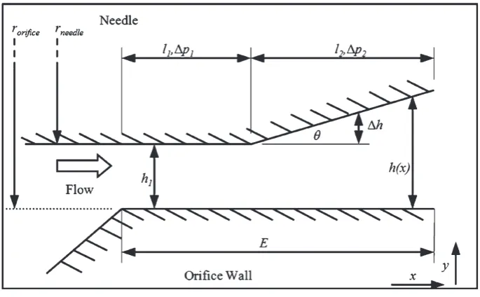
The flow channel geometry under investigation (see Fig. 1), consists of a needle with a straight (l1) and

tapered profile (l2), located within a cylindrically walled

orifice. As the needle is moved within the orifice the flow channel length varies in accordance with the level of engagement of the needle within the orifice (E in Fig. 1). The flow model has been verified against test data for flow channel heights (h1andh(x)) between 9

and 250mm andEvalues between 0 and 3.2 mm. The pressure differential across the tapered and parallel sections of the flow channel can be defined in terms of flowrateQ, taper angleh, fluid viscositym, lengths:l1,l2,h1,h(x), and mean channel

circumfer-enceW, whereW5p(ro+rn), see equation (1)

Dp~l112mQ

Wh3 1

{12m Q

W2 tanh

1

h1ztanhl2

ð Þ2{

1

h2 1

" #

ð1Þ

The first Q term represents the pressure differ-ential across the parallel section of the flow channel whereas the second Q term represents the tapered section. This can be rearranged to give the overall flowrateQ,see equation (2)

Q~1

6DpWh1

3 h21z2h1|tanh|l2ztanh2|l22

m 2l1h21z4l1l2h1tanhz2l1tanh2l22z2l2h21zl22h1tanh

ð2Þ

3 DESIGN SYNTHESIS

The design of the flow control system requires the integration of a number of elements which include: the flow channel geometry through the design of the needle and orifice profile, the needle position by means of the actuator, the actuator control algo-rithm, and the valve architecture which accounts for the linkages and construction of the valve compo-nents. Through these elements, the system design must achieve the desired flow characteristics of range, accuracy, controllability, and stability.

The flow effects of the needle profile geometry and its location in the orifice, fluid viscosity, and tem-perature are explored further. It can be seen from equation (2) that there is a cubic relationship be-tween the channel height h1and the valve flowrate.

This means that the valve characteristic is particu-larly sensitive to the orifice and needle diameters. This can be problematic as the minimum clearance between the needle and the orifice is typically be-tween 9 and 15mm, making part tolerance a critical factor in valve performance. In practical terms, this makes it very difficult and expensive to manufacture

the critical geometry of the needle valve to an accuracy which will not adversely affect the flow characteristics of the valve. As an example of the effects of valve tolerance on flowrate, a 1mm reduction in needle radius from nominal, increases flow rate by 25 per cent.

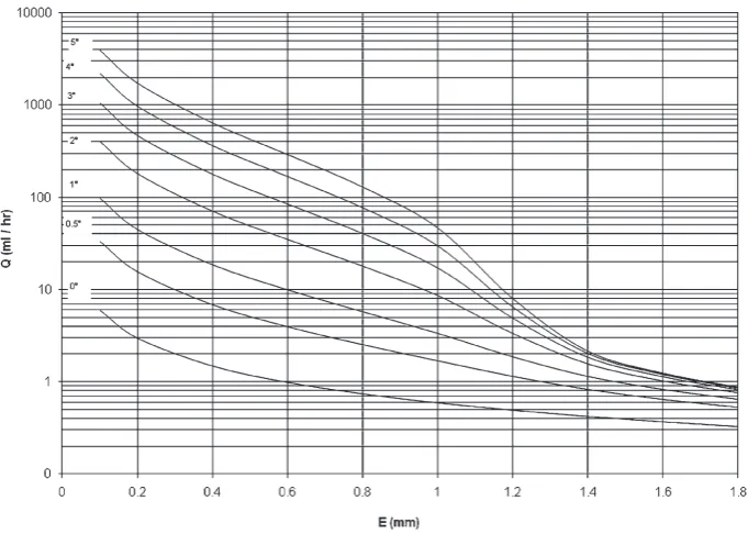
The needle profile and its relative position within the orifice determine the flow channel geometry and subsequently the valve flow characteristic. This has significant implications for the needle positioning system and control system of the valve. Figure 2 illustrates the effect on flowrate of changing the needle profile via the taper angle. It can be seen that increasing the taper angle results in a slight increase of the minimum flowrate and a significant increase in the maximum flowrate of the valve. In terms of controllability this means that there is a trade-off between fine flow control (as per a 0utaper) and a range of flows with a large taper.

It is possible to alter the needle and orifice geometry to suit different actuator and control strategies whilst essentially maintaining the flow characteristic of the valve. For example, if a high range of flow is required, this can be achieved by increasing the taper angle.

Fig. 2 Flow range is linked to the angle of the taper. The transition from composite profile to taper only occurs atE51.2 mm

However, this may lead to control stability problems as there would be an increased change in flowrate for a given change in needle position. Flowrate would then become highly sensitive to needle position and therefore increase the precision requirements of the actuator. It would also make the system sensitive to noise such as the effects of changes in ambient temperature (which is discussed later in this section). Figure 3 shows how the controllability of a 5u taper valve can be improved by increasing the orifice diameter and maximum engagement. The flow range generated by the 5u taper is maintained but the flowrate sensitivity is decreased and therefore is less susceptible to noise affecting needle engagement. Enlarging the orifice counteracts the effects of increased fluid friction caused by increasing the maximum engagement length. The increased engage-ment and similar range are clearly visible in the example shown in Fig. 3.

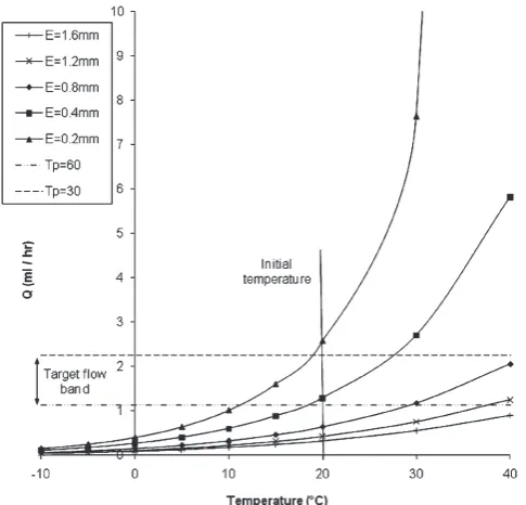
From equation (2) it can be seen that viscosity is inversely proportional to flowrate. This means that the effects of viscosity are particularly noticeable at low viscosities. In addition to this, fluid viscosity is often particularly sensitive to temperature, espe-cially in the mineral oils used for lubrication applications. This has implications for how the valve is used, as outdoor applications can see significant temperature variations over daily and yearly cycles. Using ISO32 mineral oil as an example, a 1uC change in temperature at 15uC causes a viscosity change of

about 6 per cent. Assuming a temperate climate where a daily change in temperature could be 10uC, this would result in a viscosity-induced flow change in excess of 50 per cent based on equation (2).

The valve body is also susceptible to tempera-ture changes and its effects are dependent on the valve configuration and material. The valve used in this study was arranged such that any expansion of the valve body translated directly into needle move-ment by disengaging the needle from the orifice. The valve body is 119 mm long and made of a polymer with a coefficient of linear thermal expansion of 861025mm/mm/uC. In this way, a 10uC increment in temperature would result in a valve expansion and needle movement of 0.095 mm or about 3 per cent of full travel. The temperature effect on needle position and hence on flowrate depends on the needle geometry and the engagement length but is in the region 2–5 per cent of flow rate per degree Celsius.

The temperature effects on flowrate can be illus-trated by modelling the change in viscosity and the valve expansion. Figure 4 illustrates the effects of temperature change on a valve at an initial tem-perature of 20uC. It can be seen that a change of 10uC results in a change in flowrate that is greater than the width of the desired flow band for motorcycle chain lubrication. It can also be seen that low engagement lengths (e.g. E50.2) are particularly sensitive to changes in temperature.

4 VALVE CONTROL

There are two performance criteria that an auto-mated valve control system must fulfil. The first is the ability to reach a given flowrate under a specified set of operating conditions. Whilst high-speed dyna-mic response is not normally critical for low-flow lubrication applications, it is still important for the system to be able to reach a specified flowrate within a reasonable amount of time and without unstable fluctuations. The second is the ability to maintain a given flowrate under the influence of outside disturbances such as temperature fluctuations and pressure changes.

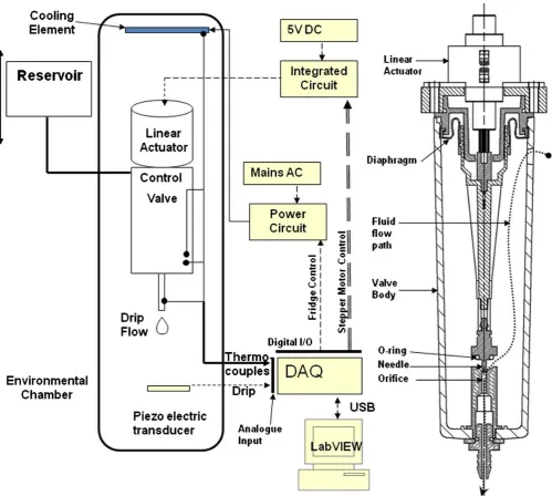
In order to develop an understanding of needle valve dynamics, a manually operated commercial valve used for motorcycle chain lubrication was modified so that the needle could be positioned using a Haydon 26000 Series, high-resolution linear actuator with travel limit switch (Fig. 5). This bipolar 5 V motor has a 7.5u step angle that translates to a linear step distance of 0.006 43 mm. Approximately 450 steps are required for full needle travel from open (step number Sn50) to closed (Sn5450). The main control profile of the needle is active at 100,Sn,420, atSn,100 the needle is not engaged with the orifice, atSn.420 the valve seal begins to seat and interrupts normal controlled flow. A stepper motor driver and valve controller was developed in

LabVIEW. This allowed the valve needle to be moved to a known position relative to the orifice whilst limiting the travel so that the valve opened and closed fully without overloading the actuator.

Flow feedback is required if a closed-loop system is to be used. A flow sensor based on the time period (Tp) between the drips from a nozzle was integrated into the test rig shown in Fig. 5. Using this apparatus, the flowrate can be inferred from the interval between drips. Drip volume was calibrated for drip intervals between 0.22 and 60 s to account for flowrate effects on drip volume. Tests conducted at 18.5, 10, and 5uC showed that drip volume is temperature-invariant.

4.1 Closed-loop control design

A closed-loop control system was developed that allows for the particular constraints of the hardware. The main features being:

(a) flow sensor: feedback from the flow sensor is available at discrete intervals and is propor-tional to the flowrate;

(b) valve actuator: the needle position is limited to dis-crete intervals due to the stepper motor actuator; (c) needle profile: the percentage change in

flow-rate per step is dependent on the engagement length of the needle.

A proportional control system was implemented by adjusting the output (actuator step number, Sn) in proportion to the error between the desired time interval Tpdand measured time intervalTpa. While

there are several types of control philosophy that can be applied to valves, such as proportional-integral-derivative and neural networks, a simple variable gain control algorithm was found to produce good results. The main elements of the closed-loop con-trol system are the linear actuated valve and the drip-interval-based flow measurement and the con-trol system must account for the particular char-acteristics of these devices. This includes the variable feedback intervals of the drip-based flowmeter, the incremental nature of the actuator, and the non-linear response of the flowrate to needle position. The closed-loop control was implemented in Lab-VIEW and used the variables:

(a) measured drip interval:Tpa;

(b) desired drip interval:Tpd;

(c) actual step number:Sna;

(d) desired step number:Snd;

(e) step correction:Snk;

(f) gain:G. Fig. 4 Valve flowrate in response to changes in

The following conditions were found to give good results.

Snd~SnazSnc ð3Þ

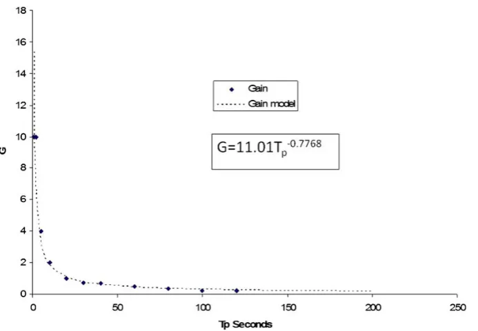
Snk~G Tpð d{TpaÞ ð4Þ

where (see Fig. 6)

G~11:01Tp{0:7768 ð5Þ

unless

Snk§50 in which caseSnk~50 ð6Þ

or

Snk¡{50 in which caseSnk~{50 ð7Þ

A suitable level of G (equations (4) and (5)) to produce a Tpaclose to that ofTpdwithout unstable

fluctuations with a reasonable response time was found by trial and error. The resulting data points were then modelled using regression to give a continuous gain range that was easily implemented in the control program.

The step correction numberSnk(equations (6) and

(7)) must be limited to damp the system in the case where large step number corrections are required. If Fig. 5 Experimental test rig incorporating linear actuated control of the valve with detail of the

there is a sudden change inTpdemand, the resulting large step change can cause unstable oscillations in needle position. There is normally sufficient damp-ing within the automatic gain controller when moving from low Tpa to high Tpd (gain is in the

region of 0.25 atTpd5100), however, any overshoot

could inadvertently cause the valve to close and therefore stop responding. Conversely, when moving from highTpato lowTpd, the gain can be as high as

15 which would cause a step correction number well in excess of permissible travel. As such, the step correction number is limited to approximately 25 per cent of full travel. There are also additional inter-ference effects from the valve itself due to the valve architecture. Moving the valve needle causes a pumping action of the diaphragm within the valve (Fig. 5), this causes a sudden peak or dip in flowrate before normal flow is re-established. The control program will react to localized peaks or troughs in the flowrate, but a fortunate effect caused by this particular valve architecture is that the peak or trough is normally in the opposite direction to the one requested. This normally has the positive effect of increasing the step correction slightly, thereby speed-ing up reaction times.

4.2 Closed-loop control testing

There are two main requirements of a valve: to reach a desired set point and to maintain that set point despite outside disturbance. Tests were devised to

gauge the ability of the valve and control system to achieve these targets.

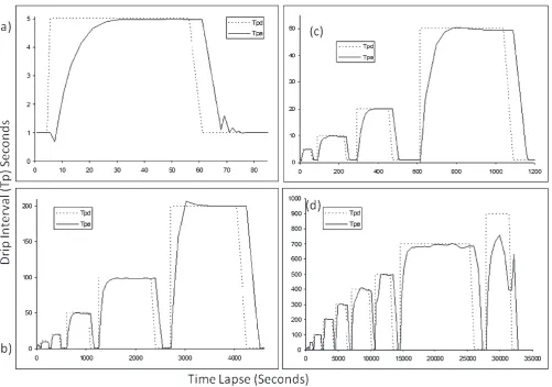
The first test consists of reaching an ever increas-ing drip interval (flow reduction) whilst returnincreas-ing to a low set-point (high flow) between each increment; in this case the low set-point isTp51 s or equivalent to approximately 80 ml/h (Fig. 7). The challenge is to be able to cope with large changes in demand at the same time as reduced feedback intervals. Very long feedback intervals can be a cause of flow instability if the control algorithm is not robust. Figure 7(a) shows a typical Tparesponse to a demand of Tpd5

5 (or approximately 13 ml/h).

The following points should be noted.

1. The system is critically damped and so overshoot is minimal or non-existent.

2. The downward response is much faster than the upwards response where damping is more evi-dent.

3. A small dip inTpajust after an upwards demand

is clearly evident and is due to the pumping effect of the diaphragm. There is a similar effect at the end of the downwards stroke, but it is not clear if this is also due to pumping effects.

4. The response lag after the demand is equal to the drip interval, i.e. 1 s atTp51 and 5 s atTp55.

From Fig. 7(b) and (c) it can be seen that the trend is consistent through ever increasing demand levels. The difference being that at higher Tpd levels, the

good match with Tpais achieved. This is due to the

increased feedback intervals and the accumulation of disturbing factors over the extended feedback period. From Fig. 7(d) it can be seen that byTp5700 the fluctuations about the set-point are more pro-nounced and that by Tp5900 the control becomes ineffective.

Above step number 400, the O-ring begins to contact the valve seat and becomes fully closed at step number 470. In this caseTpd5700 calls for step

numbers greater than 400 resulting in an unstable flow, the effects of which increase atTpd5900 to the

point where accurate control is no longer possible. Despite this, satisfactory control was achieved at

Tp5700, equal to a flow rate of 0.09 ml/h or 1 litre per 15 months. The greatest stable percentage error was 2 per cent at Tpd510, while the average error

was only 1 per cent, well within the levels required for a lubrication application and of potential use in high-accuracy applications.

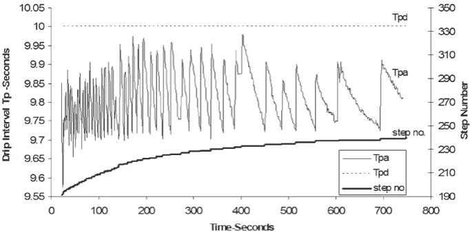
The second test investigates the systems ability to maintain a set-point while the system is disturbed by

ambient temperature change. Figure 8 shows the valve self-adjusting to compensate for a temperature rise from 5 to 20uC. The saw-tooth pattern ofTpais

caused by the reduction in drip interval caused by the rise in the ambient temperature and the cor-responding step change as the valve self-compensates. The step number can be seen rising, closing the valve to compensate for the reduction in viscosity of the fluid and the expansion of the valve body. The flow is maintained within 3 per cent of desired flowrate.

4.3 Open-loop control design

It is not always possible or practical to incorporate an inline flow sensor in a low-flow system as required for closed-loop control. In this case some form of model is required to guide the control process in terms of the main inputs. Traditional approaches to open-loop con-trol include response surface mapping to correlate the desired outcome to a number of related inputs. While it is relatively easy to implement a response surface in a control application, the difficulty lies in efficiently Fig. 7 Drip interval response compared with demand. (a), (b), and (c) show enlarged portions of

and accurately mapping the response surface to the characteristics of the physical system, and this problem intensifies as the number of control para-meters increases. Neural networks have been used in this way to capture the characteristics of a flow control system [11] although like all mapping pro-blems they require large data sets when there is a large number of control parameters. There is also the risk of over-fitting, where the mapped solution is too similar to the actual data to the extent where it is not useful for more general applications. Generating large numbers of data sets can require time-consuming and expensive tests and may not capture the full variability between different samples as required by control systems.

Reducing the data sets required to capture the full flow variability of the flow control system by using the inherent characteristics of valve flow would sim-plify and increase the accuracy of the data-fitting process. Understanding the interrelationship between the factors that affect flowrate allows the equations that represent the flow characteristics of the valve to be defined using just a few data points. The method described here uses a relatively small number of ex-perimental readings to capture the valve flow char-acteristic which is then represented in the form of a graph. This graphical representation of the valve flow characteristic can, in turn, be represented by a mathematical equation using regression. In this way it is possible to summarize the valve flow in a single equation that can be easily incorporated into a simple microprocessor for onboard control without the need for a large look-up table database.

The experimentally derived valve coefficient, Cv

[12–14], used to describe the flow characteristic of industrial control valves is used as a means of

defining flowrate in terms of differential pressure, but is used mainly for valve size selection rather than for control purposes. Thananchai [10] used a simi-lar experimental procedure to characterize the flow properties of a ball valve in terms of orifice area by plotting the flowrate in terms of pressure differential and orifice area. This was performed as part of a study to alter the flow characteristics of a valve and not used in the implementation of a control system. The minimum requirement for an open-loop control system is to be able to determine the valve position required to achieve a desired flowrate for a given pressure head at a constant temperature. The addition of the temperature variable is desirable but adds a significant level of complexity.

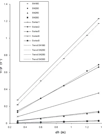
A clear pattern emerges if flowrate (represented by 1/Tpin Fig. 9) is plotted against change in pressure head (dh) and for a selection of valve positions (Sn) representing the travel range of the valve needle. As expected for negligible velocities, in agreement with Bernoulli’s principle, there is a straight line relation-ship between the flowrate and pressure head. By exploiting the linear relationship between (1/Tp) and

dh, the valve flow characteristics represented in Fig. 9 can be captured in a simple equation.

If the gradient of each step number series is calculated and called the gravity-fed needle valve coefficientGv

1=Tp~Gv|dhzj ð8Þ

wherej50 as all lines cross at the origin, then each value can be plotted against the step number in natural log form as shown in Fig. 10. This graph is the defining characteristic of the valve and as long as it can be modelled in some form, it is possible to Fig. 8 Automatic adjustment of needle position in response to a continuous increase in

predict the flowrate for any combination of valve position and pressure differential within the bounds of the initial training data. As can be seen in this example, the model is particularly straightforward due to the linear relationship between Gv and the

valve position when using a natural log scale. It takes the form

lnð ÞGv ~m|Snzk ð9Þ

where m is the gradient of the line and k is the intercept. Using equations (8) and (9) it is possible to predict the flowrate for any given valve position and pressure head, a selection of which are shown

in Fig. 9. Alternatively, it is possible to combine equations (8) and (9) and rearrange for the step number as shown in equation (10). In this way the needle position can be defined for any desired flow-rate for a given pressure head

Sn~ln ½ð1=TpÞ{j=dh�

m

{k ð10Þ

This was implemented in software and tested in an open-loop control system. A number of discrete values were predicted and checked by re-measuring flowrate and making a comparison. Average error was approximately 10 per cent of the set-point with a Fig. 9 This figure clearly shows the linear relationship between the flow variable 1/Tp and

maximum error of 25 per cent. Although 25 per cent may seem large, when considered in the context of the flow range of 1:900, this is well within the required accuracy for most lubrication applications and within the levels of expectation of accuracy for an open-loop system.

The valve coefficient profile (Gv) can be defined by

two points, which, in turn, are derived from two lines in the (1/Tp)2dhchart, each of which requires two data points. It is therefore possible to characterize the flow properties of the valve using a minimum of four data points. In practice more data points would be used to improve the reliability of the model.

5 CONCLUSIONS

The practical difficulties in reconciling flow channel geometry with analytic models makes analytic models unattractive for control purposes. However, modelling is a powerful tool for flow control system design since it allows system variables to be explored and enables the prediction of valve flow character-istics. Two methods of control have been developed: a closed-loop process and an open-loop control based on an enhanced mapping process that allows efficient mapping of valve performance and conver-sion into a form that is easily implemented in a control algorithm.

For stable operation of both open and closed-loop flow control it is necessary to consider the interac-tions between the actuator, feedback transducer and control algorithm, and flow characteristics of the needle geometry.

Based on the control system, the analytic model creates a cost relationship with the accuracy of the

system as the flow accuracy is linked to how closely the flow channel geometry matches the model inputs. It has been shown that the valve flow is particularly sensitive to the needle and orifice tolerances. Using closed-loop control removes this link as needle geo-metry is only responsible for the overall flow character-istics, while the fine adjustment of the flowrate can be accomplished by the actuator and control algorithm. It has also been shown how the needle profile can be altered to suit different actuator requirements. Alter-natively, using the enhanced mapping techniques described here means that individual valves can be efficiently calibrated for open-loop control.

A valve and control system capable of accurately controlling flow rates between 0.09 and 400 ml/hr and with a range of 900:1 was demonstrated. The control principles described here through the use of a macroscopic actuator are generally applicable and so equally relevant to microscopic counterparts.

F Authors 2011

REFERENCES

1 Oh, K. W.andAhn, C. H.A review of microvalves.

J. Micromech. Microengng, 2006,16(5), 13–39. 2 Laser, D. J.and Santiago, J. G. A review of

micro-pumps.J. Micromech. Microengng, 2004,14(6), 35–64. 3 Kidd, M. D. Bicycle chain efficiency. PhD Thesis, Department of Mechanical and Chemical Engineer-ing, Heriot-Watt University, Edinburgh, UK, 2000. 4 Stiles, G. F.Liquid viscosity effects on control valve

sizing, 19th Annual Symposium on Instrumenta-tion for the Process Industries, Texas, 1964. 5 Baumann, H. D.Viscosity flow correction for small

control valve trim. Trans. ASME, J. Fluids Engng, 1991,113(1), 86–89.

6 George, J. A. Sizing and selection of low flow control valves.InTech, 1989,36(11), 46–48. 7 Rahmeyer, W.andDriskell, L. Control valve flow

coefficients. J. Transp. Engng, 1985, 111(4), 358– 364.

8 Sondh, H. S., Singh, S. N., Seshadri, V., and Gandhi, B. K.Design and development of variable area orifice meter. Flow Meas. Instrum., 2002, 13(3), 69–73.

9 Singh, S. N., Gandhi, B. K., Seshadri, V., and Chauhan, V. S. Design of a bluff body for development of variable area orifice-meter. Flow Meas. Instrum., 2004,15(2), 97–103.

10 Thananchai, L. Design factors for ‘linear’ ball valve: theoretical and experimental studies. Songk-lanakarin J. Sci. Technol., 2005,27(2), 353–361. 11 Thananchai, L.Flow-sensorless control valve: neural

computing approach. Flow Meas. Instrum., 2003, 14(6), 261–266.

12 BS EN 60534-1:2005.Industrial-process control valves - part 1: control valve terminology and general considerations.

13 BS EN 60534-2-1:1999.Industrial-process control valves - part 2-1: flow capacity - sizing equations for fluid flow under installed conditions.

14 BS EN 60534-2-3:1998.Industrial-process control valves - part 2-3: flow capacity - test procedures.

APPENDIX

Notation

Cv valve coefficient

dh pressure head (m)

E needle engagement (m)

G gain

Gv gravity-fed needle valve coefficient

l1,l2,h1,h2 lengths (m)

p pressure (N/m2)

rn needle radius (m)

ro orifice radius (m)

Sn step number

Sna actual step number

Snd desired step number

Snk step correction

Tpa measured drip interval (s)

Tpd desired drip interval (s)

Q volumetric flowrate (m3/s)

W channel circumference (m)

h taper angle (deg. rad.)