The Variation of Software Survival Time for Different Operational Input Profiles

City, University of London Institutional Repository

Citation

:

Bishop, P. G. (1993). The Variation of Software Survival Time for Different

Operational Input Profiles. Fault-Tolerant Computing, 1993. FTCS-23. Digest of Papers., The

Twenty-Third International Symposium on, pp. 98-107. doi: 10.1109/FTCS.1993.627312

This is the accepted version of the paper.

This version of the publication may differ from the final published

version.

Permanent repository link:

http://openaccess.city.ac.uk/14345/

Link to published version

:

http://dx.doi.org/10.1109/FTCS.1993.627312

Copyright and reuse:

City Research Online aims to make research

outputs of City, University of London available to a wider audience.

Copyright and Moral Rights remain with the author(s) and/or copyright

holders. URLs from City Research Online may be freely distributed and

linked to.

City Research Online: http://openaccess.city.ac.uk/ [email protected]

The Variation of Software Survival Time for

Different Operational Input Profiles

(or why you can wait a long time for a big bug to fail)

P. G. Bishop Adelard, Coborn House, London, E3 2DA, England

Abstract—This paper provides experimental and theoretical evidence for the existence of contiguous failure regions in the program input space (‘blob’ defects). For real-time systems where successive input values tend to be similar, blob defects can have a major impact on the software survival time because the failure probability is not constant. For example, with a ‘random walk’ input sequence, the probability of failure decreases as the time from the last failure increases. It is shown that the key factors affecting the survival time are the input ‘trajectory’, the rate of change of the input values and the ‘surface area’ of the defect (rather than its volume).

I. INTRODUCTION

This paper is an extension of earlier experimental studies on the failure characteristics of some known software defects [1], [2], [3]. The results of these studies cast doubt on the general validity of an assumption of constant probability of failure for software. In conventional reliability theory, it is often assumed that an item fails with a fixed probability per unit time (λ), and the mean interval between failure is

1/λ. When this assumption was tested experimentally, it was found that the failure probability was not constant for some input distributions. This variability could be explained by an assumption of defects which occupy contiguous regions of the input space (‘blobs’). The paper begins by summarizing some of the relevant reliability theory together with the main results of the earlier study. The remainder of the paper presents evidence to back up the assumption of ‘blob’ defects and presents a more detailed analysis of effect of ‘blobs’ on failure behaviour.

II. SOMERELEVANTRELIABILITYTHEORY

Software reliability theory differs from conventional theory because it operates in discrete rather than continuous time [4]. Most software operates on an input-process-output cycle, so failures are only meaningful in terms of software execution cycles rather than absolute time. In this paper the ‘time unit’ is deemed to be one execution cycle.

In this study we are primarily concerned with embedded operational software where repair is infeasible in the short term or where transient failures (‘glitches’) occur which are hard to diagnose. In these circumstances, software operation is a sequence of ‘successes’ and ‘failures’ for successive execution cycles. This sequence can be analysed to derive:

λ the mean probability of failure per exe-cution

λS(n) the instantaneous probability of failure

aftern successful executions

λf(n) the instantaneous probability of failure

aftern failed executions

Note that survival intervals are measured from the first suc-cessful execution cycle, which could be the first execution of the program, or the first successful execution after a succession of failure cycles.

The calculation of λ is simply the ratio of failure cycles to total cycles.λS(n)is calculated by deriving the probability

density functionP(NS ≥n)whereNSrepresents the survival

interval in program execution cycles. The instantaneous failure probability aftern successful cycles is computed as:

λS(n) =

P(NS =n)

P(NS ≥n)

This hazard function is simply the ratio of periods that survive exactlyncycles (i.e. fail on cyclen+ 1) against total number of periods that reach n cycles. λf is calculated in a

similar way.

The above analysis applies whether the failure rate is constant or fixed. Of course if the software failure rate is constant then, for all n >0:

λ=λS(n) =λf(n)

While direct measurements of λS are feasible, it is often

difficult to get sufficient accuracy. As an alternative, the distributionP(NS ≥n)can be compared with the distribution

expected for the constant failure rate assumption. If we assume that the probability of failure per execution of the program is a constant, λ0, then survival interval probability follows a

Bernoulli distribution, where the probability of observing a survival interval ofncycles or more is:

P(NS > n) = (1−λ0)n

and the probability of surviving exactlyncycles is:

P(NS =n) =λ0(1−λ0)n

III. SUMMARY OFEARLIERWORK

function specified by the UK Atomic Energy Authority. The failure rate behaviour of the various faults was examined for two types of random input data.

The first set of tests used totally arbitrary data; input values were randomly selected from a uniform distribution for each program input. The observed survival time distribu-tion matched an assumpdistribu-tion of constant failure rate to 95% confidence. The failure rate for sequences of failures (λf(n))

were also analysed. For around half the faults, there was a 95% confidence fit to an assumption of constant failure rate. However the remaining faults exhibited avariableλf(n). This

was explained by the fact that these particular faults damaged the ‘internal state’ of the program (variables used from one cycle to the next).

The second set of tests attempted to be more realistic. In most real-time applications (and certainly for this particular application) the input values do not change greatly from execution cycle to the next. We chose to model this by performing a ‘random walk’ over each set of input values. On each execution, all the input parameters were altered by a random ‘step’ which was a small percentage of the input range. While λwas very similar to the uniform random case, the survival interval density distribution could no longer be expressed as a Bernoulli distribution. However the distribution was found to be a good fit to a power law:

P(NS =n) =A.n−k

where 1.2 < k < 1.8 for the different faults examined. Translated back in terms of λS(n) this meant that chance

of failure decreased rapidly as n increased. At first this was extremely puzzling, but thinking back to the idea of a ‘defect’ in the program domain a credible explanation was obtained. Evidence existed to support the theory that a program fault creates a ‘blob’-shaped defect in the state space (i.e. the individual points of the defects are close to each other) [5], [6], [7]. If this were true for the PODS defects, then it was clear that the probability of failure would no longer be constant. Immediately after recovery from a failure, the program operating point is close to a defect. As the number of steps without failure increases, the mean distance from the defect is increased so it is plausible that the probability of failure for subsequent steps is reduced.

To get a more analytic explanation of this phenomenon we turned to the theory of coin tossing [8]. Coin tossing is analogous to a simple linear model of a program state space where positive and negative steps replace heads and tails, and the cumulative winnings represent the distance from the defect. Using this theory, the probability of returning to the defect after nfailure-free steps is:

P(NS =n) =A.n−1.5

which was close to the observed behaviour. However it is clear that this model is not a complete explanation because it is easy to show that the mean survival interval will be infinite after an infinite number of steps. This arises because the simple model assumes an infinite linear program state space. In practice the program operating point is constrained to move within a finite input range. If a program survives long enough to traverse

the complete input range, the mean distance from the defect should tend to a fixed value. Thus the probability of failure per execution is likely to become constant. For a random walk, the mean distance moved from the start point is s√n where

nis the number of steps andsis the mean step length. Thus the complete rangershould be traversed when:

n= (r/s)2

As an example, for a mean step length of 10%, the full range should be traversed in 100 steps. Experiments to check this hypotheses confirmed the factλS(n)stabilized after this point.

However it was noted thatλS(n)was much less thanλ.

It was clear that further work was needed to both to justify the hypothesis that the software defects were indeed ‘blobs’ in the input space of these programs, and to investigate the impact of blobs on failure behaviour in general. The remainder of the paper describes an investigation into these aspects.

IV. EXPERIMENTALJUSTIFICATION OFBLOBDEFECTS

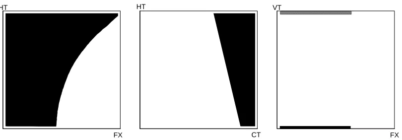
The TRIPC and TRIPV test harnesses were both adapted to plot out the software failure regions in 15 two-dimensional slices of the input space around a detected failure point. The experiment showed that all the defects in the TRIPC and TRIPV programs occupied contiguous regions of the input space. Some two-dimensional views of typical faults are shown in figures 1 to 3. It can be seen that the term ‘blob’ is not particularly appropriate since the shapes are often angular and elongated. An analysis was made to establish the factors affecting the shapes of the faults and a number of factors were identified.

A. Input Variable Dependency

One factor which emerged clearly from this analysis was that a bug which has a quite low overall failure rate can look quite large when viewed as a series of two-dimensional slices through the input space. For example TRIPV fault 9 (figure 1) has a failure rate of 10−4 per cycle under uniform random test conditions, but occupies a significant fraction of the input range in some dimensions. This occurs when the fault is only dependent on one or two of the input variables. The values of the remaining variables do not contribute to the failure. Since the one or two key variables are kept constant at the point of failure when plotting the remaining two-dimensional slices, these plots are completely black (i.e. a faulty result is returned whatever input values are selected). Hence it is actually the plots containing thesmallestdefect regions which tend to contain the variables most likely to activate the bug.

B. Dependency on Combined Input Variables

For other faults, the faulty computed output variable(s) depend on a higher proportion of the input variables combined according to some equation. For these faults, the failure regions tended to be more similar in size and skewed with respect to the axes. TRIPC Fault 10 is an example of this (see figure 2).

This particular fault is readily explained since the main analogue input variables are combined using linear and non-linear equations to compute a reactor power (see figure 4). If contour lines of constant reactor power are drawn through the input space, they are skewed with respect to all the axes which affect the calculation. Any faults within or ‘downstream’ of this calculation tend to have edges aligned with these contours.

C. Effect of Error Masking

One notable feature of the analysis was the effect of error masking. This effect has been noted in earlier studies [3]. In essence, quite large internal errors can result in much smaller external failures because some downstream program logic corrects the error. Simple examples of this are:

• the OR of several binary values – where a correct ‘1’ value overrides any number of faulty inputs.

• Range-clipping – where an analogue value is clipped within a maximum and minimum range. Faulty internal values can be clipped to the correct external value. Both of these error-masking functions are present within the PODS reactor trip example (see figure 4).

One example of error-masking can be seen in TRIPC Fault 19 (figure 3). This causes a failure in the out-of-range signal (RE) . The RE signal is formed from the OR of several out-of-range indications. Whenever any correct out-of-range indication is generated, it masks the faulty input to the OR logic. This causes straight portions to be sliced off the failure region close to the upper and lower boundaries of the input dimensions.

V. THEORETICALJUSTIFICATION FORBLOBDEFECTS

All 30 defects analysed in the two diverse programs were ‘blobs’; similar faults have also been observed by other re-searchers [5], [6], [7], so there is strong experimental evidence on the existence of blob defects. Admittedly, the PODS application is fairly simple and many of the defects are quite large faults which were detected during development and are therefore atypical the faults remaining in operational software. This section presents a supporting theoretical justification for the existence of blob defects. Furthermore I will argue that the general shapeof such defects should be predictable.

Any computation can be regarded as the composition of a set of functions. The data flow diagram for the PODS application (figure 4) illustrates this. For a function computing analogue values, it is probable that failures occur over contigu-ous ranges of input values. Typical reasons for this might be:

• Incorrect positioning of the boundary between two types of calculation.

• Missing boundaries.

• Incorrect table values.

• Inadequate calculation precision (e.g. for small values). • Algorithm approximations.

Provided the functions ‘upstream’ and ‘downstream’ of the faulty function are smooth continuous functions, the observed failure regions will also be contiguous. More generally, each function is a mapping between a domain and a range, for example the ‘program’f maps the input domainsAandB to the output domainP, i.e:

(A×B) →f P

This might be implemented as the following composition of functions, shown schematically below:

A →f1 X

× →f3 Z →f4 P

B →f2 Y

If we replace f1 by a faulty function f10 there will be a

failure subset Af ⊂A for which incorrect values in X will

be generated. It might be assumed that the observed failure regionF in the program input space will be:

F =Af×B

However this presupposes that all the values in Af ×B

will generate incorrect final values. This can be the case when the downstream functions all have one-to-one mappings. However most practical programs condense information rather than expand it, and this implies that many-to-one mapping functions are more likely to be used. In this case ‘error masking’ can occur which has the of cutting off portions of the original failure region. A simple example of this is where f3

implements the MAX function. Whenever theyvalue exceeds thexvalue, thecorrectvalue ofzis computed. More formally, the other functions in the program constitute a ‘failure mask’

MAB ⊂A×B and the observablefailure region is:

Fobs= (Af×B)∩MAB

A many-to-one mapping function ‘upstream’ of an error region has a different effect. For example, if there was an erroneous single point inZ, this would ‘project back’ through the inverse mapping function f₃−1 to many points in the do-mainX×Y. If the function is continuous, the ‘projected back’ single point becomes a contour in the domain X ×Y. Take the simple example where f3 implements the ‘+’ function,

the back-projected contour satisfies the equation x+y =z0

wherez0is the erroneous value. Shifting the single point to an

adjacent value shifts the contour in a direction at right-angles to the contour. So a contiguous range of error values in Z

projects to a solid diagonal band inX×Y. In general, if the back-projection space has a large number of extra dimensions compared to the error, the contour becomes a hypersurface. A contiguous range of values in the error domain generates a hypersurface of finite thickness which is probably skewed with respect to dimensions of the input space. Any non-linearity in the upstream functions, f1 and f2, will further distort the

hypersurface when it is projected back to the input space

masking in downstream computations (e.g.f4). So the overall

failure regionZf when observed at the input space would be:

Fobs= (f1×f2)−1 f3−1 (Zf ∩MZ)

To some extent therefore, it should be possible to predict the shape of a defect (if not the thickness normal to the surface). The shape should align with contours of equal value for the function upstream from the fault. In addition we should be able to predict the boundaries of any masking functions which can truncate this error region.

The difficulty of predicting the actual defect shape increases with the complexity of the application. Complex functions feeding into further complex functions can lead to very distorted contours of equal output value. If the upstream mapping functions are many-to-one anddiscontinuousor non-monotonic, a contiguous error range for a faulty internal func-tion may map backwards into multiple and entirely distinct regions in the input space (i.e. there can be many ‘blobs’ for one software defect). Thus a simple internal error region can be distorted and replicated when its image is projected back on to the input space (like viewing a simple object through a multi-faceted distorting lens).

The overall conclusion is that the shape of the fault depends more on where the fault is located (in a functional sense) within the program. Thus the likely defect shape at a particular program point might also be deduced by ‘seeding’ an artificial defect at that point. In addition it is reasonable to expect a failure region to:

• be a hypersurface of finite thickness with some edges aligned with contours of equal output value for the function upstream of the error.

• exhibit sharp angles where the failure regions have been truncated by down-stream masking functions.

VI. IMPACT OFBLOBS ONSOFTWAREFAILURE

Having demonstrated that ‘blob’ defects are likely to occur in software, the impact of this observation was explored in greater detail. It is clear that key factors in the failure behaviour of the software will be:

• the input distribution

• the ‘trajectory’ through the input space • the actual shape of the blobs.

A. Effect of the Input Distribution

It is well-known that mean failure rate λ will be affected by the distribution of input values. Specific input values are either faulty or correct, so altering the activation probability for an input value will clearly change the overall failure rate. However the existence of ‘blobs’ may well result in a greater sensitivity to changes in the input distribution. The distribution of operational input values will cover a subset of the input space which may or may not coincide with the blobs in the input failure region. If the operational distribution is close to blob, even a small shift in the distribution could alter the proportion of the failure region that is covered hence changing

λvery significantly.

B. Effect of Trajectories

For a given input distribution, it is possible to have many different types of trajectory, from totally random to entirely deterministic. For a trajectory that proceeds in small ‘steps’ through the input space, the software survival time can be regarded as the ‘transit time’ between the blobs. For a given trajectory of lengthd, executed in steps of mean lengths, the mean transit time (or mean time of continuous success) will be

tS=d/s

Note that d can be very large since it is possible to traverse the input range many times before hitting the fault. In practice there will be a distribution of different trajectories of different lengths, but for a fixed distribution of trajectory lengths, it is clear that:

tS ∝1/s

A similar argument can be applied to the times of continuous failure,tF, i.e.

tF ∝1/s

This implies that the mean time for continuous success,

tS, is actually proportional to the rate of change of the

input variables. Thus if the ‘external world’ conditions change more rapidly, the interval between failures will decrease. One possible interpretation of this phenomenon is that software is more likely to fail just when you need it, i.e. when the external conditions are changing rapidly.

Note that this apparently counter-intuitive behaviour is consistent with the idea of a mean rate of failure per execution cycle, λ, that stays the same. From the definitions of tS and

tF it is clear that:

λ=tF/(tS+tF)

because this represents the ratio of the failure time to the total time. SincetS andtF maintain a fixed ratio,λremains

unchanged as sis varied.

C. Effect of Defect Shape

For a deterministic or semi-deterministic trajectory, the volume of a defect does not have such a dominant effect on the survival time; it is actually the effectivecross-sectional areaof the defect that is most important. The effective cross-sectional area can vary depending the direction of the trajectory. For example, a pencil-shaped defect has very different cross-section when viewed end-on or sideways. The distribution of trajectories across the surface also affects the effective cross-section. For a random walk motion, the whole surface area of the defect contributes to the effective cross-sectional area, since the trajectories are even distributed in all directions. With such evenly distributed trajectories, the effective cross-sectional area is directly related to the surface area of the de-fect. However for any given set of trajectories, some effective mean cross-sectional area,A0 should exist, so:

tS ∝1/A0s

step is large enough. This will occur if the width of the blob,

wi, is smaller than the step,si in any dimension of the input

space i. The relationship derived above has to be qualified:

tS∝1/A0s, si< wi for alli

If the mean step length si becomes greater thanwi, the blob

becomes ‘semi-transparent’. In the limit, the mean transit time (tF) through the defect will be one execution cycle. Hence

from the earlier equation:

tS≈(1−λ)/λ, si>> wi for any i

D. Survival Interval Distribution

The previous analysis applies regardless of the specific trajectories employed. Furthermore, only the mean success interval (tS) has been examined. Now the impact of trajectories

and blobs on the distribution of survival intervals (P(NS ≥

n)) will be examined. The key item of interest is whether the

very factof survival can provide any further information about the chance of further survival. We have chosen the measure

M T CS(n), which is the mean time for continued survival. This measure takes the mean of all survival periods for which

NS ≥ n and subtracts the prior survival time (n−1). This

definition implies that tS =M T CS(1).

For uniform random input data, the prior survival time is irrelevant. The probability of failure remains constant, so for all n:

M T CS(n) =tS =

1−λ λ

For a deterministic trajectory, the probability of failure in-creases as the number of steps increases, so assuming an exponentially distributed set of trajectory lengths, one would expect a relationship of the form:

M T CS(n) =tSe−K0(n−1)

Finally in the ‘random walk’ case, the fact of survival after a failure increases the chance of being further away from a defect, so the probability of failuredecreaseswith the number of cycles. However, when the number of cycles is sufficient to span the complete input range (i.e. nmax > 1/s2i) in all

dimensions, there is no possibility of moving further from the defect, so the distribution of any surviving operating points in input space becomes stationary, resulting in a constant probability of failure.

The very fact of survival tells us that the program operating point is outside the blob. After a sequence of successes, failure is only possible when the program operating point lies within a small ‘skin’ with a thickness of one step si around the

blob. Assuming that the defect lies in an unit input space, the instantaneous failure probability is:

λS(nmax)∝

X

i=1,k

ρiAisi, nmax>>1/s2i

whereρis the probability of the program operating point lying within the ‘skin’, k is the number of dimensions, and Ai is

the surface area of the defect normal to dimension i.

With a stationary input value distribution, ρ is constant. However the actual value of ρ varies with the step size. A

simulation to derive the stationary distribution for different step lengths showed there was an approximate relationship of:

ρ∝s

for the density of program operating points within the ‘skin’. Assuming the step length is identical in all dimensions, we obtain the approximate relationship:

λS(nmax)∝As2

where A is the total surface area of the defect. It follows that, approximately:

M T CS(nmax)∝

1

As2

VII. SIMULATIONSTUDY

The results of the above analysis are quite a surprising; for uniform random input sequences, it is volume of the defect that matters, but for other types of input trajectory thesurface area that affects the survival time. In addition the rate of change of input data affects the survival time. So very long survival periods are possible even with very large faults. This is consistent with the experimental observations made in the earlier random walk study.

To check the predictions made by this analysis, a series of random walk simulations were made using n-dimensional defects for different values of n. The input space was of unit length in each dimension, and the defect was located at the centre of the unit space with an identical length in each dimension. The program operating point started at the defect boundary, and the failure sequences were recorded and analysed to obtainM T CS(n)andM T CF(n).

Figure 5 shows the distribution ofM T CS(n)of a 0.1 vol-ume linear defect for different step lengths. The very large 0.3 length step approximates to a uniform random distribution and

M T CS(n)remains virtually constant. For steps smaller than 0.1 (the width of the defect), it can be seen that M T CS(1)

increases as 1/s with the step length and M T CS(n) rises asymptotically to a value which is approximately proportional to1/s2_.

Figure 6 plots the distribution of M T CS(n) at a fixed step length, for defects with the same volume but different dimensions (and hence surface area). It can be seen that

M T CS(1)can differ by an order of magnitude for differently shaped defects. This ratio remains roughly the same for all values of n, which would be expected if M T CS(n) was proportional to the surface area.

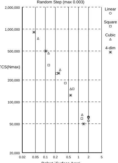
Figure 7 plots M T CS(nmax) against surface area for

differently shaped defects. It can be seen thatM T CS(nmax)

for differently shaped defects with the same surface area is roughly the same. The relationship is probably not exact be-cause higher order defects have quite large linear dimensions. For example, a four-dimensional defect with a volume of10−2, has linear dimensions of 0.31. This ‘squeezes’ the available space (making the effective step size bigger). This ‘squeeze effect’ is less significant for smaller surface areas and better agreement can be seen. It can also be seen thatM T CS(nmax)

defect. Again the ‘squeeze effect’ for large surfaces, together with different stationary distributions at the ‘corners’ of higher order defects are likely to cause deviations from the simple inverse relationship.

VIII. DISCUSSION

It is clear from the analysis and simulation results that ‘blobs’, combined with correlated input sequences, can have a dramatic effect on the survival characteristics of software. As an example, in one simulation run using a maximum step of 3% per cycle and a defect occupying 10% of the input space, that the mean time for continued survival at first successful execution, M T CS(1), was over 100 execution cycles. After a survival period of 100 cycles (i.e. n=100)M T CS(n)rose to more than 1000 execution cycles, and the asymptotic value of M T CS(n) was over 5000 execution cycles. The results would be even more pronounced with smaller step sizes.

Assuming the overall results are valid there are a number of practical implications to what, to date, has just been a theoretical exercise. With the blob model, failures are likely to come in ‘bursts’ interspersed by long periods without failure. During a failure, restarting the software will have little effect if the input conditions are similar, the system could be unavailable for far longer periods than might be expected.

If the input conditions change more rapidly, the intervals of continuous success or failure shorten. This could have unfortunate consequences. Given that the software is working successfully (which should be the norm) the time to failure will be long when conditions are stable (e.g. flying straight and level), and shorten just when you need them (e.g. aborting a landing, etc).

On the other hand, the same property could be useful for final system and reliability testing. For some real-time systems a few execution failures are sufficient to cause a failure of the entire system (e.g. a dynamically unstable aircraft). In this case the actual length of the failure ‘burst’ is irrelevant, but the length of the survival time is of great relevance (especially to the pilot). In these circumstances, it may be legitimate to argue that system testing using input data with far larger steps than normal (up the credible limit for blob size) is a form of accelerated testing. Time has effectively been speeded up by the use of larger steps. Thus the survival time estimate obtained in accelerated testing can be ‘scaled up’ in inverse proportion to the step size to gain an estimate for the mean survival time under the expected operational conditions.

Some reliability estimation methods [9], [10], [11] assume a constant failure rate over time for any given set of faults and input distribution, This study indicates the failure rate will vary, so current reliability estimation methods may need to be modified to take account of the effect of ‘blob’s.

The shape of blobs may be relevant to software diversity. Previous theoretical work [12], [13] has shown that diverse programs will exhibit correlated failures if some input values are more ‘error prone’ than others. The analysis of blobs shows that that similar internal ranges of error may back-project to cover very different amounts of the input space, so some portions of input space are more error-prone. Thus a priori

predictions of ‘error proneness’ and failure correlation should be possible.

IX. SUMMARY ANDCONCLUSIONS

This study has shown that:

• The hypothesized ‘blob’ defects were present in the PODS application programs.

• On theoretical grounds, such blobs are likely to exist in any program and, to some extent, the general shape of the fault can be predicted from the program function and the location of the fault within the program.

• The existence of ‘blob’ defects implies that a constant failure rate assumption is not justifiable, especially for when successive input values are strongly correlated (as they are in many real-time systems).

• By definition, the mean times for continuous success and failure (tS and tF) maintain a fixed ratio for a given

mean failure rate. However the existence of ‘blob’ defects combined with correlated input sequences (trajectories) can lead to some surprising results:

– For small enough trajectory steps, tS is inversely

related to the cross-sectionalareaof the ‘blob’ and the step length.

– For random walk sequences, if a program sur-vives n cycles, the mean continued survival time,

M T CS(n), increases as n increases. In the limit, for largen,M T CS(n)tends to an asymptotic value which is inversely proportional to the blob surface area and thesquareof the step length.

– For deterministic trajectories M T CS(n) decreases

with increased survival periods.

If these results are generally valid, it has some interesting implications for the likely failure behaviour of software-based systems. In particular:

1) Failures are likely to come in ‘bursts’ interspersed by long periods without failure.

2) Given that the software is operating successfully, the chance of continued operation is greatly improved if there are only small changes in input conditions (e.g. flying straight and level in an aircraft).

3) Conversely failures become more likely if there are major changes in the external conditions (e.g. take-off, landing, evasive action).

4) It may be possible to justify ‘accelerated testing’ using large rates of change, where the measured survival time can be scaled in proportion to the maximum rate of change expected in normal operation.

5) Software reliability theory may need to be modified to take account of the effects of ‘blobs’.

Acknowledgements

This work was undertaken at Adelard as part of the SHIP project (EV5V 103, the Assessment of the Safety of Hazardous Industrial Processes in the Presence of Design Faults) which has financial support from the CEC in the framework of Major Industrial Hazards.

REFERENCES

[1] P.G. Bishop,et al,PODS – A Project on Diverse Software, IEEE Trans. Software Engineering, Vol SE-12, No 9, 1986.

[2] P.G. Bishop and F.D. PullenProbabilistic Modelling of Software Failure

Characteristics, IFAC SAFECOMP 88, Fulda, Germany, Nov 1988.

[3] P.G. Bishop and F.D. Pullen,Failure Masking: A Source of Dependency

in Multi-version Programs, Paper in: Dependable Computing and Fault

Tolerant Systems, Vol 4. ”Dependable Computing for Critical Applica-tions”, (ed. A. Avizienis and J.C. Laprie), Springer Verlag, Wien-New York, 3-211-822249-6, 1991.

[4] A.A. Salvia and R.C. Bollinger, On Discrete Hazard Functions, IEEE Trans. Reliability, Vol 31, No 5, 1982.

[5] J.C. Knight and S. BrilliantGraphs of Failure Regions in the Input Space, private communication, 1986.

[6] P.E. Amman and J.C. Knight,Data Diversity: An Approach to Software

Fault Tolerance, IEEE Trans. Computers, Vol 37, No 4, April 1988.

[7] G. Finelli,NASA Software Failure Characterisation Experiments Relia-bility Engineering and System Safety, Vol 32, 1991.

[8] W. FellerAn Introduction to Probability Theory and its ApplicationsJohn Wiley and Sons, New York, 1957.

[9] W. Ehrenberger and K. Pl¨ogert,Statistical Verification of Reactor

Pro-tection Software, International Symposium on Nuclear Plant Control,

Cannes, April 1978.

[10] D.L. Parnas, A.J. van Schouen and Shu Po Kwan,Evaluation of Safety

Critical SoftwareComm. ACM, Vol 33, No 6, June 1990.

[11] C.W. Ramamoorthy and F.B. Bastani,Software Reliability - Status and

Perspectives, IEEE Trans. Software Engineering, Vol SE-8, No 6, 1981.

[12] D.E. Eckhardt and L.D. Lee, A Theoretical Basis for the Analysis

of Multi-version Software Subject to Coincident Failures, IEEE Trans.

Software Engineering, Vol SE-11, No 12, 1985.

[13] B. Littlewood and D. Miller, A Conceptual Model of the Effect of Diverse Software Methodologies on Coincident Failures in Multi-Version

Software, Proc. Third Int. Conference on Fault-Tolerant Computing

GT

CT GF

VT HT

FX

VT FX HT

HT

FX CT

HT VT

FX

CT GF

Fig. 1 TRIPV Defect 9 (2-d Slices through the Failure Region)

Fig. 2 TRIPC Defect 10 (2-d Slices through the Failure Region)

Operator Inputs Plant Inputs

Staticise Input

Power

Calculation

Range

Clip

Trip

Logic

Trip Outputs

Conversion OR

OR

OR

Diagnostics

(Linear Defect, volume 0.100)

1 10

100 1,000

10,000 100,000

1,000,000

Observed successes (N) MTCS(N)

0.003

0.01

0.03

0.1

0.3

Step

1 10 100 1,000 10,000 100,000 1,000,000

Step

Step

Step

Step

Fig 4. PODS Trip Example Fig. 5 MTCS(N) for Different Step Sizes

Volume 0.003, Random Step (max 0.003)

1 10

100 1,000

10,000 100,000

1,000,000 1

10 100 1,000 10,000 100,000 1,000,000

Observed successes (N) MTCS(N)

Cubic Square

Linear

Random Step (max 0.003)

0.02 0.05 0.1 0.2 0.5 1 2 5 20,000

50,000 100,000 200,000 500,000 1,000,000 2,000,000

Defect `Surface Area' MTCS(Nmax)

Linear

Square

Cubic

4-dim