City, University of London Institutional Repository
Citation: Becerra, V.M. (1994). Development and applications of novel optimal control algorithms. (Unpublished Doctoral thesis, City University London)
This is the accepted version of the paper.
This version of the publication may differ from the final published version.
Permanent repository link: http://openaccess.city.ac.uk/8377/
Link to published version:
Copyright and reuse: City Research Online aims to make research outputs of City, University of London available to a wider audience. Copyright and Moral Rights remain with the author(s) and/or copyright holders. URLs from City Research Online may be freely distributed and linked to.
City Research Online: http://openaccess.city.ac.uk/ publications@city.ac.uk
DEVELOPMENT AND APPLICATIONS OF
NOVEL OPTIMAL CONTROL ALGORITHMS
By
Victor Manuel Becerra
A THESIS SUBMITTED FOR THE DEGREE OF DOCTOR OF PHILOSOPHY
CONTROL ENGINEERING RESEARCH CENTRE DEPARTMENT OF ELECTRICAL, ELECTRONIC
AND INFORMATION ENGINEERING
CITY UNIVERSITY, LONDON
To
TABLE OF CONTENTS
Page
T ABLE OF CONTENTS . . . 3
LIST OF TABLES . . . 9
LIST OF FIGURES . . . 10
ACKNOWLEDGMENTS . . . 13
DECLARATION . . . 1..+
ABSTRACT . . . 15
LIST OF SYMBOLS . . . 16
LIST OF ABBREVIATIONS . . . 21
CHAPTER 1. INTRODUCTION . . . 22
1.1 Control systems in industrial processes . . . . . 22
1.2 System identification and adaptive control. . . 24
1.3 Optimisation of industrial processes . . . . . . 24
1.4 Predictive control . . . 26
1.5 Dynamic optimal control . . . 27
1.6 ISOPE algorithms . . . 29
1.7 Scope and aims of the thesis ... . . . .. 30
1.8 Outline of the thesis . . . . . . . 33
1.9 Summary . . . 35
CHAPTER 2. CONTINUOUS TIME DISOPE ALGORITHM . . . 37
2.1 The optimal control problem . . . 37
2.1.1 Problem formulation . . . 38
2.1.2 Necessary optimality conditions . . . 39
2. 1.3 Linear-Quadratic optimal control . . . 40
2.2 Dynamic ISOPE . . . . . . . ..+2
2.2.1 Problem formulation and solution . . . ..+3
2.2.2 Performance index augmentation . . . 48
2.2.3 Terminal state constraints . . . .. 50
2.3.2 Terminal state constraints . . . 53
2.3.3 DISOPE algorithm with LQ model-based problem . . . 55
2.4 Simulation examples . . . . . . . . . 57
Example 2.4.1: Continuous stirred tank reactor (CSTR) . . . 58
Example 2.4.2: Third order nonlinear system . . . 63
2.5 Summary . . . 67
CHAPTER 3. DISOPE WITH CONSTRAINED CONTROLS . . . 68
3.1 Optimal control with input-dependent constraints . . . 68
3.1.1 Problem formulation . . . 68
3.1.2 Necessary optimality conditions (the minimum principle) 69 3.2 Dynamic ISOPE approach . . . 70
3.2.1 Problem formulation and solution . . . 70
3.3 Case of simple bounds on the controls . . . 73
3.4 Simulation examples . . . 74
Example 3.4.1: Continuous stirred tank reactor (CSTR) with bounded control . . . 75
3.5 Summary . . . 79
CHAPTER 4. HIERARCHICAL DISOPE ALGORITHM . . . .. 81
4.1 Large-scale systems and hierarchical control . . . 81
4.2 Problem formulation and solution approach . . . .. 82
4.3 Case with Linear-Quadratic model-based problem . . . 88
4.3.1 Formulation . . . 88
4.3.2 Hierarchical DISOPE algorithm with LQ model-based problem . . . 90
4.4 Simulation example . . . 92
Example 4.4.1: Seventh order nonlinear system . . . 93
4.5 Summary . . . 101
CHAPTER 5. DISCRETE-TIME DISOPE ALGORITHM . . . 102
5.1 Digital computer control . . . .. 102
5.2 Discrete-time DISOPE algorithm . . . .. 102
5.2.2 Performance index augmentation . . . .. 109
5.2.3 Terminal state constraints . . . .. 110
5.3 Case with Linear-Quadratic model-based problem . . . 111
5.3.1 Formulation . . . 111
5.3.2 Terminal state constraints . . . .. 113
5.3.3 Discrete-time DISOPE algorithm with LQ model-based problem · . . . .. 115
5.4 Exact discretization of continuous time systems . . . .. 117
5.5 Simulation examples. . . . .. 117
Example 5.5.1: Nonlinear discrete-time system . . . 118
Example 5.5.2: Continuous stirred tank reactor (CSTR) with bounded control . . . . . . . .. 122
Example 5.5.3: CSTR with bounded control and terminal constraints · . . . 126
5.6 Summary . . . 128
CHAPTER 6. SET-POINT TRACKING DISOPE ALGORITHM . . . 130
6.1 Tracking optimal control . . . .. 130
6.2 Set-point tracking DISOPE algorithm . . . . .. 130
6.2.1 Formulation in discrete time 130 6.3 Incremental control weighting . . . 135
6.4 Simulation examples . . . . .. 135
Example 6.4.1: Exothermal CSTR . . . .. 136
6.5 Summary . . . 144
CHAPTER 7. HANDLING OF STATE DEPENDENT CONSTRAINTS WITHIN THE DIS OPE FRAMEWORK . . . 146
7.1 Formulation . . . . . . . .. 146
7.2 Simulation examples. . . .. 150
Example 7.2.1: Linear system with time-varying state constraint
· ... .
150CHAPTER 8. APPLICATION OF DISOPE IN THE OPTIMISATION OF BATCH
PROCESSES . . . .. 155
8.1 Batch processes . . . .. 155
8.2 DISOPE approach . . . 156
8.3 The Shadow Model concept . . . 158
8.4 Estimation of derivatives. . . .. 159
8.5 Choice of the dynamic model for the optimisation step . . . .. 159
8.6 Choice of the algorithm for solving the model-based problem . .. 160
8.7 Simulation examples. . . . . . . . . . . .. 161
Example 8.7.1: Batch chemical reactor. . . .. 161
8.8 Summary . . . 166
CHAPTER 9. APPLICATION OF DIS OPE IN NONLINEAR PREDICTIVE CONTROL . . . 167
9.1 Predictive control . . . 167
9.2 Nonlinear predictive control . . . 170
9.2.1 Formulation . . . 170
9.2.2 Nonlinear predictive control algorithm (NLP-DISOPE) . 172 9.3 Dynamic optimisation algorithm . . . 174
9.3.1 Choice of the LQ model-based problem in set-point tracking DISOPE . . . 174
9.3.2 Handling of control magnitude constraints . . . 174
9.3.3 Handling of state dependent constraints . . . 174
9.3.4 DIS OPE algorithm initialization (nominal solution) . . .. 175
9.4 State/parameter estimation algorithm . . . 175
9.4.1 Extended Kalman Filter . . . . . . . .. 175
9.4.2 Kalman Filter tuning . . . 177
9.5 Simulation examples. . . .. 178
Example 9.5.1: Exothermal CSTR . . . 178
Example 9.5.2: Exothermal CSTR with parametric uncertainty 182 Example 9.5.3: Exothermal CSTR under load disturbance ... 185
Example 9.5.4: Optimisation of two CSTR in series . . . 187
9.6 Summary . . . 191
CHAPTER 10. ~OVEL DEVELOPMENTS IN STEADY-STATE PROCESS
OPTIMISATION USING DYNAMIC INFOR,\1ATION . . . 192
10.1 Linear state-space model identification schemes . . . .. 192
10.2 Preliminary assumptions . . . 195
10.3 Initial formulation . . . .. 195
10.3.1 First order necessary optimality conditions of SSOP .. 197
10.3.2 First order necessary optimality conditions of RHDOP. 198 10.4 First approach: DSSO, a steady state optimiser . . . 199
10.4.1 Steady-state optimality of a RHDOP controller with N=l . . . 199
10.4.2 Development of a steady-state optimiser based on the above analysis . . . 202
10.4.3 Analysis of the converged Algorithm 10.4.2 when the control is saturated . . . .. 205
10.4.4 DSSO Algorithm with rate constraints . . . . . . .. 206
10.4.5 Comments on the structure of the control law . . . .. 207
10.5 Second approach: Long range prediction with a linearized state-space model of the process (DISOPE as a steady-state optimiser) . . . 208
10.5.1 Formulation . . . 209
10.5.2 Optimality . . . 212
10.5.3 Practical considerations . . . 216
10.5.4 A link between LP-DISOPE and DSSO . . . 217
10.6 Simulation studies . . . 218
Example 10.6.1: Second order nonlinear system . . . 218
Example 10.6.2: Optimisation of a multicomponent distillation column . . . . I I I
---Example 10.6.3: Optimisation of two CSTR in series . . . 23-+10.7 Remarks . . . 238 10.8 Summary . . . .. 2-+0
CHAPTER 11. COMPARISONS OF DISOPE WITH OTHER ALGORITHMS
...
11.1.1 Comparison between DISOPE and the quasilinearization approach . . . 2-.+2
11.1.2 Comparison with previous work by Hassan and Singh (1976) . . . 2-.+3
11.1.3 Comparison with previous work by Mahmoud et al (1980)
. . . 248
11.2 Summary . . . .. 253
CHAPTER 12. CONCLUSIONS ... . . . .. 254
12.1 Conclusions . . . .. 254
12.2 Suggestions for further research . . . .. 258
REFERENCES . . . 260
APPENDIX . . . 269
A. Derivation of Procedure 2.3.1 269 B. Derivation of Procedure 2.3.2 271 C. A conjugate-gradient optimal control algorithm. . . .. 274
D. Derivation of Procedure 5.3.1 . . . . .. 278
E. Derivation of Procedure 5.3.2 . . . .. 280
F. Derivation of Procedure 6.2.1 287
LIST OF TABLES
Table No. Page
2.4.1: Algorithm's performance for example 2.4.1 . . . 60
2.4.2: Algorithm's performance for example 2.4.2 . . . 64
3.4.1: Performances for example 3.4.1 . . . 77
4.4.1: Performances for example 4.4.1 . . . 96
5.5.1: Algorithm's performance, example 5.5.1 5.5.2: Algorithm's performance, example 5.5.2 5.5.3: Algorithm's performance, example 5.5.3 119 123 126 6.4.1.1: Description of cases in example 6.4.1 . . . . .. 138
6.4.1.2: Algorithm's performance, example 6.4.1 . . . .. 138
7.2.1.1: Tuning parameters for example 7.2.1 . . . 151
7.2.1.2: Performances for example 7.2.1 . . . . . . .. 152
8.7.1: Performances for example 8.7.1 . . . 163
9.5.1.1: Example 9.5.1, controller performance . . . 180
9.5.2.1: Extended Kalman Filter tuning parameters for example 9.5.2 . . . . .. 182
9.5.3.1: Extended Kalman Filter tuning parameters for example 9.5.3 . . . 185
9.5.4.1: Extended Kalman Filter tuning parameters for example 9.5.4 . . . . .. 190
10.6.1.1: Optimal results obtained using DSSO and MA TLAB' s optimisation toolbox . . . 220
10.6.2.1: LP-DISOPE tuning parameters . . . .. 223
10.6.2.2: DSSO tuning parameters . . . . . . . . .. 223
10.6.2.3: Identifier tuning parameters . . . . .. 224
10.6.2.4: Results obtained as compared with the design case and the MTS method
...
22510.6.3.1: DSSO tuning parameters . . . .. 235
10.6.3.2: LP-DISOPE tuning parameters. . . . . . . .. 235
LIST OF FIGURES
Figure No. Page
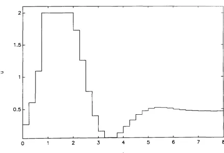
2.4.1.1: Example 2.4.1, final state vector . . . 60
2.4.1.2: Example 2.4.1, final and nominal control signals . . . . . . . 61
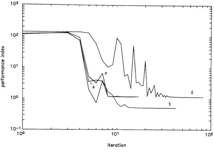
2.4.1.3: Example 2.4.1, convergence of the real performance index . . . 61
2.4.1.4: Example 2.4.1, convergence of the control variation norm. . . 62
2.4.2.1: Example 2.4.2, final state response . . . 65
2.4.2.2: Example 2.4.2, final control signals . . . 65
2.4.2.3: Example 2.4.2, convergence of the control variation norm, cases (a) and (b) . . . 66
3.4.1.1: Example 3.4.1, final control signal . . . 78
3.4.1.2: Example 3.4.1, Convergence of the performance index . . . 78
3.4.1.3: Example 3.4.1, control variation norm versus iterations. . . 79
4.3.2: Information exchange in Algorithm 4.3.2 . . . 92
4.4.1.1: Example 4.4.1, subsystem 1 state vector . . . 97
4.4.1.2: Example 4.4.1, subsystem 2 state vector . . . 97
4.4.1.3: Example 4.4.1, subsystem 3 state vector . . . 98
4.4.1.4: Example 4.4.1, subsystem 1 final control signal . . . 98
4.4.1.5: Example 4.4.1, subsystem 2 final control signal . . . 99
4.4.1.6: Example 4.4.1, subsystem 3 final control signal . . . 99
4.4.1.7: Example 4.4.1, control variation norm vs. iteration (hierarchical case)
...
1004.4.1.8: Example 4.4.1, interaction norm vs. iteration (hierarchical case) '" 100 5.5.1.1: Example 5.5.1, final state response . . . .. 120
5.5.1.2: Example 5.5.1, final control vector. . . .. 120
5.5.l.3: Example 5.5.1. control variation norm vs. iterations . . . .. 121
5.5.1.4: Example 5.5.1 performance index vs. iterations . . . 121
5.5.2.1: Example 5.5.2, final state response . . . .. 12.+
5.5.2.2: Example 5.5.2, final control signal 12.+ 5.5.2 . .3: Example 5.5.2, control variation norm VS. iterations . . . .. 125
5.5.2.'+: Example 5.5.2 performance index VS. iterations . . . 125
5.5.3.1: Exan1ple 5.5 . .3. final state response. . . .. 127
5.5.3.2: Example 5.5.3, final control signal . . . .. 127
5.5.3.3: Example 5.5.3, control variation norm vs. iterations . . . . . . .. 128
6.4.1.1: Example 6.4.1.a, dimensionless temperature and set-point 6.4.1.2: Example 6.4.1.b, dimensionless temperature and set-point 139 140 6.4.1.3: Example 6.4.1.e, dimensionless temperature and set-point . . . .. 140
6.4.1.4: Example 6.4.1.a, final control signal . . . .. 1.+ 1 6.4.1.5: Example 6.4.1.b, final control signal. . . .. 1.+ 1 6.4.1.6: Example 6.4.1.e, final control signal . . . 1.+2 6.4.1. 7: Example 6.4.1, control variation norm vs. iterations . . . . .. 1.+2 6.4.1.8: Example 6.4.1, performance index vs. iterations . . . .. 143
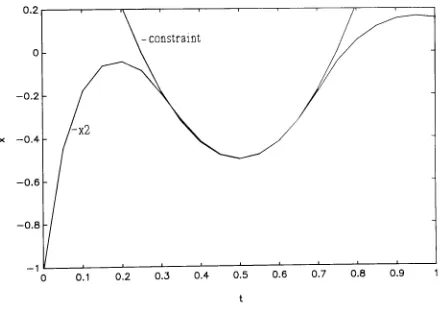
7.2.1.1: Example 7.2.1, constrained state and constraint . . . 152
7.2.1.2: Example 7.2.1, final control signal . . . 153
7.2.1.3: Example 7.2.1, control variation norm vs. iterations . . . 153
7.2.1.4: Example 7.2.1, penalized performance index vs. iterations . . . .. 154
8.7.1.1: Example 8.7.1, final concentration responses . . . .. 164
8.7.1.2: Example 8.7.1, final temperature profile . . . 164
8.7.1.3: Example 8.7.1, control variation norm vs. iterations . . . 165
8.7.1.4: Example 8.7.1 performance index vs. iterations . . . 165
9.2.1: Predictive control approach . . . 169
9.2.2: Schematic diagram of the controller . . . 173
9.5.1.1: Example 9.5.1, dimensionless temperature and set-point . . . 180
9.5.1.2: Example 9.5.1, control signal . . . 181
9.5.1.3: Example 9.5.1, number of DISOPE iterations per sample interval .. 181
9.5.2.1: Example 9.5.2, dimensionless temperature and set-point, case (a) . .. 183
9.5.2.2: Example 9.5.2, dimensionless temperature and set-point, case (b) . .. 183
9.5.2.3: Example 9.5.2, parameter estimate, case (b) . . . lR.+ 9.5.2.4: Example 9.5.2, control signal case (b) . . . .. 184
9.5.3.1: Example 9.5.3, dimensionless temperature and set-point. cases (aL (b)
...
1869.5.3.2: Exan1ple 9.5.3, parameter estimate, case (b) . . . 186
9.5.3.3: Example 9.5.3, control signal for cases (a) and (b) . . . 187
10.1: Simplified diagram of shadow model approach for plant dynamic optimisation · . . . .. 194 10.6.1.1: Example 10.6.1, control signals
10.6.1.2: Example 10.6.1, state trajectory
220 221 10.6.1.3: Example 10.6.1, evolution of the performance index . . . 221 10.6.2.1: Example 10.6.2.a, Top vapour flow rate trajectory . . . 225 10.6.2.2: Example 10.6.2.a, concentration of methane trajectory . . . 226 10.6.2.3: Example 10.6.2.a, condenser temperature controller set:-point . . . .. 226 10.6.2.4: Example 10.6.2.a, reboiler temperature controller set-point . . . 227 10.6.2.5: Example 10.6.2.a, top pressure controller set-point . . . .. 227 10.6.2.6: Example 10.6.2.a, evolution of the steady-state objective function . 228 10.6.2.7: Example 10.6.2.a, top vapour flow rate predicted and actual trajectories · . . . 228 10.6.2.8: Example 1 0.6.2.a, concentration of methane predicted and actual trajectories · . . . 229 10.6.2.9: Example 10.6.2.a, predicted and applied condenser temperature controller set-point . . . .. 229 10.6.2.10: Example 10.6.2.a, predicted and applied reboiler temperature controller set-point . . . .. 230 10.6.2.11: Example 10.6.2.a, predicted and applied top pressure controller set-point · . . . 230 10.6.2.12: Example 10.6.2.b, top vapour flow rate trajectory . . . .. 231 10.6.2.13: Example 10.6.2.b, concentration of methane trajectory . . . 231 10.6.2.14: Example 10.6.2.b, condenser temperature controller set-point .... 232 10.6.2.15: Example 10.6.2.b, reboiler temperature controller set-point . . . 232 10.6.2.16: Example 10.6.2.b, top pressure controller set-point . . . 233 10.6.2.17: Example 10.6.2.b, evolution of the steady-state objective function 233 10.6.2.18: Example 10.6.2, schematic diagram of the process . . . 234 10.6.3.1: Example 10.6.3.a, trajectory of concentration of B in the second reactor
·
...
"... .
23610.6.3.2: Example 10.6.3.a, control signals, temperatures in reactors 1 and 2 237 10.6.3.3: Example 10.6.3.b, trajectory of concentration B in the second reactor
· ...
" " " " " " . " " " " . " " " .. " " " " ... "..
" " " " " " ".
"..
" " " ... " " 23710.6.3'-+: Example 10.6.3.b, control signals, temperatures in reactors I and 2 23X
ACKNOWLEDGMENTS
I wish to express my sincere gratitude to my research supervisor, Prof. Peter David Roberts, for his guidance, advice, understanding and kindness given throughout this work. His professionalism and high standards have provided me with a source of inspiration.
I am indebted to Mr. G.W. Griffiths and Dr. 1. Lin from SAST Ltd. for the interest they showed in my project, for their valuable suggestions and for having allowed me to implement new developments using the facilities at SAST and to test them using industrial scale process simulations.
I am grateful to the following organizations for their financial support which made this project a reality:
*
CEPET (Centro de Formacion y Adiestramiento de Petroleos de Venezuela y susFiliales).
*
SAST Ltd., U.K. (Special Analysis and Simulation Technology).*
Gilchrist Educational Trust, U.K.Special thanks to Mrs. 1. Rivellini from City University, for her kindness and caring attitude.
DECLARA TION
The author grants power of discretion to the University Librarian to allow this thesis to be copied in whole or part without further reference to him. This permission covers only single copies made for study purposes only, subject to normal conditions of acknowledgement.
ABSTRACT
The main concern of this thesis is to advance and improve the existing knowledge of a dynamic optimal control technique known as DISOPE. so as to make it attractive on one hand for its implementation in the process industry and, on the other hand, as a novel nonlinear optimal control algorithm. The main feature of the technique is that it has been designed so as to achieve the correct optimum of the process in spite of inaccuracies in the mathematical model employed in the computations.
Several extensions of the basic continuous time DIS OPE technique are proposed in this work. For the development of the algorithms, emphasis is placed on making the techniques implementable in digital computer based industrial process control problems. These extensions include discrete-time. and set-point tracking versions, extensions for handling control and state dependent inequality constraints. and a hierarchical version.
Applications of DISOPE are proposed in the following areas: nonlinear predictive control, predictive optimising control based on adaptive state-space linear dynamic models, and batch process optimisation.
All the algorithms and techniques proposed in this thesis have been implemented in software and tested with relevant simulations. These studies include dynamic simulations of low order chemical reaction systems and studies on the dynamic optimisation of an industrial-scale multicomponent distillation column using a rigorous process simulator.
Symbol
n
m
n o u x f*
f
L* L J*J m
H* H p <p A B
Q
(Q)R (R)
ex
y
LIST OF SYMBOLS
Description
Order of the system
N umber of control inputs
Number of output variables
Control vector
State vector
Initial state vector
Real state mapping
Model-based state mapping
Real performance measure function
Model-based performance measure function
Real performance index
MOP performance index
EOP performance index
MMOP performance index
Real Hamiltonian
Model-based or augmented Hamiltonian
Costate vector
Terminal weighting function
Model-based system matrix
Model-based control distribution matrix
Intermediate state weighting matrix (augmented)
Control weighting matrix (augnlented)
Terminal state weighting matrix
State related time-varying parameter vector
Performance related time-varying parameter
z
v
-A (-A)
-~ (-~) t k k(t) S h G g
w
F vr ,
k \'
k :
k
I'
£ \'
C(li,t)
State separation vector
Control separation vector
Costate separation vector
Lagrange multiplier vector
Lagrange multiplier
Lagrange multiplier vector (augmented)
Lagrange multiplier vector (augmented)
time
time index
time interval
discrete time interval
Continuous time Riccati matrix
Continuous time Riccati vector
Discrete time Riccati matrix
Discrete time Riccati vector
State feedback gain matrix
Driving input vector
Time varying matrix
Time varying matrix
Lagrange multiplier
Control convexification factor
State convexification factor
Control relaxation gain
State relaxation gain
Costate relaxation gain
Control con\'crgcnce tolerance
u . , mm U max
SAT, sat
S. I W. I M .. I) Q. I y
sex)
c
J (]
p
P
£
k r
A, B
F*
t I
N
('N.N
{'Set of admissible control trajectories
Control bounds
Saturation functions
State distribution mapping i-th subsystem
Interactions distribution mapping i-th subsystem
Interaction input vector for i-th subsystem
Coupling matrix from subsystem j to subsystem i
Interaction distribution matrix i-th subsystem
Lagrange multiplier for interactions, i-th subsystem
Convergence tolerance for interactions
Output vector
Output mapping
Output matrix
Output reference trajectory
SCROP performance index
SCROP performance measure function
State dependent constraint mapping
Penalty factor
Smoothed penalty relaxation function
A small scalar value
Convexification gain factor
Estimated jacobian matrices
Estimated state vector
Continuous state mapping
Continuous time variable
Control horizon
Prediction horizon
J r Receding horizon performance index d y Prediction error
G
f Noise distribution matrix
Ym Measured output W
p Process noise vector
V m Measurement noise vector
Qf Process noise covariance matrix
R
f Measurement noise covariance matrix
Xo Expected value of initial state
Po Initial state covariance matrix
AI' Cf Jacobian matrices
K
f Kalman gain A
9 Vector of estimated parameters
A
90 Expected value of initial parameter vector
Po Parameter vector covariance matrix
11 Pseudo-noise vector
Q
O Pseudo-noise covariance matrixN u Moving horizon identifier update period
Nd Moving horizon identifier data length
q -I Backward shift operator A(q -I) Polynomial matrix
B(q -I) Polynomial matrix
C(q -I) Polynomial matrix
AI' BI ,
C
I Matrix polynomial coefficientsN* Steady state objective function
<t> Linear terminal weighting vector
A* , B* Exact jacobian matrices
9\n n-dimensional real space
I n Identity matrix of order n
x
VH x
[aH]
T=
[aH ... aH]
T whereH
and Xj are scalarsax
aXI
aX
nafl
afl
aXI
ax
naf
where
f.
and x. are scalarsax
I Jaf
naf
naXI
ax
nAbbreviation ISOPE DISOPE ROP MOP EOP MMOP SCROP EKF DMC MAC GPC PID LQ LQG SSOP RHDOP DSSO NLP-DISOPE LP-DISOPE MTS CDC CPU mIn lim
LIST OF ABBREVIATIONS
Description
Integrated system optimisation and parameter estimation Dynamic ISOPE
Real optimal control problem
Model-based optimal control problem Expanded optimal control problem
Modified model-based optimal control problem State constrained real optimal control problem Extended Kalman Filter
Dynamic Matrix Control Model Algorithmic Control Generalized Predictive Control Proportional-Integral-Deri vati ve Linear -Quadratic
Linear -Quadratic-Gaussian
Steady-state optimisation problem
Receding horizon dynamic optimisation problem Steady-state optimiser based on dynamic information Nonlinear predictive DIS OPE
Linear predictive DIS OPE Modified two step method Central difference formula Central processing unit Minimize
CHAPTER 1
INTRODUCTION
1.1 CONTROL SYSTEMS IN INDUSTRIAL PROCESSES
The purpose of control systems is to influence physical processes in such a way that certain control objectives may be achieved. Such control objectives reflect the goals of the industry which operates the process. Those goals are usually related to product quality, safety, economics, environmental regulations and operational constraints.
A physical process is a combination of operations carried out to change something in the physical world. Processes are characterized by their input and output elements in ternlS of matter, energy and information. An industrial process outputs products from raw materials and energy input. The input information to a process is a set of variables that influence or control the behaviour of the process. The output information of a process is a set of measured variables that characterize the operation of the process. Factors which cannot be manipulated but influence the process are called disturbances and they reflect the effects of the surrounding environment. The undesirable effects of external disturbances on the process must be suppressed. Control systems are used to achieve this.
Many processes are essentially unstable and must be equipped with control systems to ensure stable and, hence, safe and reliable operation.
Product quality and economic goals are of paramount importance. An industrial process should produce the desired amounts of the final products with certain minimum levels of quality. Also, the operation of the plant must correspond with the market conditions. Further, the operation should be as economical as
possible in its use of energy, raw materials and labour.
Quality and economics can be defined by means of optimisation. The most comnlon form of optimisation is steady-state optimisation, in which the optimum operating points are calculated and sent to the control systems as reference values
such optimum set-points. Often, the econOmIC objectives which are pursued by optimisation yield optimum operational conditions which lie at the intersection of
process constraints. Such constraints arise due to physical limitations inherent to process equipment and their operation, safety considerations and environmental regulations. Thus control systems should be able to take into account constraints in some way.
In the last few decades, there has been a rapid development in the field of digital computers and microelectronics. The application of digital computers in process control has evolved from the pioneering works in the 1950' s to becoming a standard technique for implementation of new control systems in the 1980' sand 90' s. This involves from single loop controllers to large-scale distributed control systems. Digital computers are also being used increasingly as means for the design and analysis of control systems.
During the 1930' s proportional-integral-derivative (PID) controllers first appeared. They were originally implemented using pneumatic technology and have passed through several development stages. Today, most new PID controllers are
implemented digitally. They are the standard tool for solving process control problems. They are relatively easy to tune and no explicit model of the process model is required. In the presence of process nonlinearities a change in operating conditions may produce loss of performance of the PID controller. The presence of
time-delays and multiple interacting control loops complicates the tuning process and may also limit controller performance. Today PID controllers which possess
o
automatic tuning capabilities are becoming increasingly popular (Astrom and
Hagglund, 1988).
In the model-based approach for control, a process model is developed which
1.2 SYSTEM IDENTIFICATION AND ADAPTIVE CONTROL
System identification is the field of mathematical modelling of systems from experimental data. It has acquired widespread applications in many areas. In control engineering system identification methods are used to obtain appropriate models for the design of control systems and simulation (Soderstrom and Stoica, 1989).
Ever since the beginning of systematic controller design there has been the problem of finding the proper controller structure and parameters for a given process. Another difficulty has been the fact that the controller must perform well for a range of operating points. Automatic adjustment of the controller parameters was first proposed in the 1940' s. The term adaptive control was first used at that time (lsermann et ai, 1992).
Given a process model structure, on-line system identification may be integrated with controller design. Thus, the parameters of the identified model and the performance requirements of the system are used in a controller design stage in order to obtain the controller parameters. The controller parameters may be updated on-line. This gives rise to a class of adaptive controller called self-tuning controller. In this class of adaptive controller the uncertainty in the estimated parameters of the process model is not accounted for in the controller design stage (Astrom and
Wittenmark, 1989).
1.3 OPTIMISATION OF INDUSTRIAL PROCESSES
The process industry has experienced important changes during the last few decades due to the increased costs of energy and raw materials, and increasingly strict environmental regulations. It is believed that emphasis should be on improving efficiency and increasing profitability of existing plants rather than on plant expansion (Edgar and Himmelblau, 1988). To achieve such a goal, one of the most
important means is optimisation.
Moreover, the computing power required for implementing such systems has been made available at reasonable prices during the last decade (Balchen and Mumme.
1988).
Steady-state process optimisation, often named optimising control, can be
situated within the functional hierarchy of the overall plant management and control system at a level called supervisory control.
The economic objective which is pursued by steady-state optimisation IS usually the maximisation of net profit, given the product demand, prices of final products, raw materials, energy, equipment wearing, pollution taxes, operational costs, etc.
The basis for optimising control is the economic objective which is quantified by means of a performance index (or objective function), a (steady-state) mathematical model of the plant and knowledge of the relevant process constraints. The result from steady-state optimisation is a set of optimal controller set-points. at which the process should be regulated until a change in economic parameters determines a new optimum operating point.
Optimising control is particularly common in large integrated process systems (oil refineries, petrochemicals, etc.).
Dynamic optimisation is more complicated. It takes into account the dynamic behaviour of the process and intends to manipulate the input of the process during transient conditions in such a way that some dynamic criterion is optimized. Hence, a dynamic model of the plant is required. Dynamic optimisation is often termed
optimal control.
Dynamic optimisation may be applied in the process industry, for instance. In the following cases which are directly related with economic objectives
(Rijnsdorp, 1991):
*
Optimisation of total process run, In cases when process behaviourdeteriorates with time.
*
When switching continuous processes from one mode of operation to another.trying to minimize the amount of off-specification product.
*
Optimisation of the operation of batch processes. seeking to maximize. for*
When disturbances with economic impact have a frequency such that the process rarely reaches steady state.However, dynamic optimisation with econorruc objectives is not widely applied in the process industry (Arkun and Stephanopoulos, 1980). Some reasons for this are (i) dynamic models are more difficult to develop than steady-state models: (ii) The solution of a dynamic optimisation problem is far more complicated and time consuming than steady state optimisation. The latter is becoming less important due to the increasing computer power becoming available at decreasing prices.
One particular class of dynamic optimisation, with regulatory rather than economic objectives, is a technique called LQG (linear-quadratic-gaussian). This is an established method for the design of multivariable control systems which has the advantages that the input-output pairing problem is avoided, for the structure of the controller is given by the design; stability is guaranteed if the model is perfect, and it may easily handle systems with time-delays and non-minimum phase behaviour (Anderson and Moore, 1989). Nevertheless, this technique has not become popular in the process industry because a good process model is required, and hence lacks robustness. Additionally, it may not handle constraints explicitly. For a survey of LQG applications in the process industries see the paper by Johnson (1993).
1.4 PREDICTIVE CONTROL
A particular technique which has been widely applied within the last two
decades in the process industry is Predictive Control based on linear input-output models of the plant. Predictive control belongs to the class of model-based controller design concepts, because a model of the plant is used to compute the control action. Some well known predictive controllers are Dynamic Matrix Control, DMC (Cutler and Ramaker, 1979), and Model Algorithmic Control, MAC (Richalet {'( ai, 1978).
The reasons for their acceptance are many, but the main ones are: they are easy to tune: they nlay handle systematically process constraints. multi variable processes and time delays: knowledge of future set-point changes can be included: their
conlputational requirenlents are modest (Soeterboek, 1992: Garcia et ai, 1989).
Linear predictive controllers, such as DMC, have been extended to handle input and output constraints (Garcia and Morshedi, 1986) and some of them, such as
Generalized Predictive Control (GPC) have adaptive features (Clarke et ai, 1987).
Predictive controllers implement dynamic optimisation in a receding-horizon
framework. If the objective is to follow a set-point, the process model is linear, the performance index is quadratic, and in the absence of process constraints, then predictive controllers allow a relatively simple analytical solution. Otherwise, iterative methods have to be used (Mayne and Michalska, 1990).
There have been growing interest in the last few years on extending predictive control concepts to take into account process nonlinearities. Some of those schemes have been presented in the literature (Sistu and Bequette, 1991: Gattu and Zafiriou, 1992; Balchen et ai, 1992). A common characteristic is their increased computational load. Most of them are based on nonlinear state space models of the process and some of them include state and parameter estimation to give robustness, adaptability, and stability to the controller. If the dynamic optimisation scheme allows for general performance index specifications, economic criteria can be included (Balchen et ai, 1992).
1.5 DYNAMIC OPTIMAL CONTROL
Optimal control theory is the mathematical tool used for addressing and solving dynamic optimisation problems.
In the seventeenth century Bernoulli studied the brachistocrone problem and then initiated the classical calculus of variations. After three centuries of developments, optimal control theory has been formalized as a general extension of the calculus of variations. It has developed into a very mature field and it has attracted the attention of numerous researchers from very diverse disciplines. Many
solutions to optimal control problems. Thus, algorithms implemented on digital computers have to be used.
The classical tool for solving optimal control problems is the calculus of variations. However, it cannot deal with control magnitude constraints. Two yery important developments were Pontryagin's minimum principle (Pontryagin et ai,
1962) and Bellman's dynamic programming (Bellman and Dreyfus, 1962). The minimum principle solves problems without control constraints in a similar way to the calculus of variations. However, the method is more general because it can work with control constraints. Dynamic programming can handle control and state constraints. Its main disadvantage is the so called "curse of dimensionality" which implies that the approach requires too much computer memory even with relatively low order problems.
Numerous algorithms have been proposed in the last two decades for solving optimal control problems. It is not the purpose to review here all of them. Nonetheless, it is worth mentioning a rather general classification according to the approach used for the solution:
*
Function space algorithms: The necessary optimality conditions obtained from the application of the maximum principle are enforced iteratively in some way. Some examples here are quasilinearization methods, function space gradient algorithms, variation of extremals methods (Bryson and Ho,1975~ Sage & White, 1977~ Kirk, 1970).
*
Parametrization methods: Here control (and sometimes state) variables are parametrized in an approximated way (usually in terms of basis functions) and then the objective function is minimized (or maximized) by using finite dimensional mathematical programming (Sisirena and Tan, 1974~ Sargent and Sullivan, 1978~ Teo et ai, 1991 ~ Biegler, 1984).Key algorithmic issues are convergence rates, memory requirements, computational load, handling of constraints, suboptimality, handling of large-scale systems and numerical precision.
Provided the dynamic model is linear, the performance index is quadratic (in terms of state and control variables) and constraints are absent, then the optin1al control problem has a relatively straightforward non iterative solution usually based
on the solution of matrix differential (or difference) equations. This is a very important particular case of optimal control problems and is usually termed as LQ (linear-quadratic) optimal control (Anderson and Moore, 1989; Lewis, 1986a).
1.6 ISOPE ALGORITHMS
As has been mentioned in Section 1.2 the optimal set-points calculated by steady-state optimisation are based on a mathematical model of the controlled plant. Because, in general, the model will not be a faithful representation of the real physical process, the set-points so obtained will only be optimal for the model and not for the real plant. Moreover, the process operates in an environment which keeps changing. Hence it is important to provide the mathematical model of the process with some adaption.
In order to take into account differences between the mathematical model and the real process a technique called the two-step method has been proposed. Here the steady-state model contains parameters which are estimated by comparing model-based and measured outputs. Then the system optimisation and parameter estimation problems are treated separately and solved repeatedly until convergence is achieved. However, there is interaction between the optimisation and parameter estimation problems and the solution so obtained will be, in general, suboptimal. The reason for this lies in the fact that inadequate output derivative information (with respect to the manipulated variables) from the plant is used in the model-based optimisation.
In order to allow for the interaction between parameter estimation and system optimisation, the interacting variables are separated and, as a consequence, a modifier is introduced in the model-based optimisation. This modifier takes into account differences between the real process and model-based output derivatives with respect to the manipulated inputs. This enables the iterative technique to achieve the correct optimal operating point of the real process in spite of model-reality differences. This technique was originally introduced by Roberts (1979) and is called integrated
system optimisation and parameter estimation (ISOPE).
have been rigorously investigated (Brdys and Roberts, 1987). Several simulations and laboratory pilot-plant implementations have been carried out and the utility of the technique has been demonstrated. Furthermore, on-line implementation on large-scale process plants seems very likely in the near future (Lin and Griffiths. 1992: Griffiths et ai, 1993).
Since the origin of the ISOPE technique its extension to dynamic optimisation has been suggested (Roberts, 1979). More recent works have also recommended such an extension (Amini-Largani, 1990). In recent research by Roberts (1992) a dynamic extension of ISOPE has been introduced. It has been termed DISOPE (Dynamic-ISOPE) and, as an extension, the philosophy behind the techniques remains very similar. However, DISOPE is in itself a new technique with a different range of applications. It can be considered as a distinctive field of research. Furthermore, as it has been mentioned in Section 1.2, dynamic optimisation is more complicated.
The development of novel optimal control algorithms, mainly new extensions of the DISOPE approach, and the study of their potential applications in process control have been the central areas of research of the doctoral work described in this thesis.
1.7 SCOPE AND AIMS OF THE THESIS
As it was mentioned in Section 1.5 ISOPE is a well established technique for optimising control of industrial processes. Dynamic ISOPE, on the other hand, is
relatively recent.
As it was originally developed and published (Roberts, 1992), DISOPE addressed continuous-time, unconstrained, centralized and time invariant optimal
control problems.
The central aIm of this thesis is to advance and Improve the existing knowledge on the technique so as to make it attractive on one hand for its implementation in the process industry and, on the other hand, as a novel nonlinear optimal control algorithm. Additionally, as a result of research work carried out during the project, a new technique for steady-state process optimisation based on dynamic information (DSSO) has been developed.
*
*
*
*
*
*
*
*
The means through which the central objective is to be achieved are:
To develop discrete-time versions of DIS OPE so as to make it suitable for digital computer on-line implementations.
To extend the DISOPE technique to handle control and state dependent constraints.
To develop hierarchical extensions of DISOPE so as to make it applicable in large-scale systems.
To extend the DISOPE algorithm for taking into account reference trajectories which should be tracked.
To investigate the ways the techniques developed can be applied in the process industry, particularly in the fields of nonlinear predictive controL batch process optimisation and predictive optimising control.
To implement in software the algorithms developed and to test their performance through simulation studies.
To investigate the ways the inherent flexibility of the DISOPE approach can be exploited.
To compare the structure and performance of DISOPE with other existing techniques.
The scope and original contributions of this thesis are briefly summarized
below.
Contribution to algorithm development
Several DISOPE control algorithms have been developed. This contribution includes theoretical derivation, development of implementable versions and actual software implementation of: discrete time, set-point tracking, hierarchical, control
constrained, state constrained and receding horizon DISOPE algorithms. Emphasis has been given to make the technique suitable for industrial implementation. Furthermore, a steady-state optimiser based on dynamic information (DSSO) has been developed, implemented in software and tested with simulation examples.
Contribution to DISOPE approach flexibility exploitation
performance indexes have been developed and investigated. This includes: (i) the use of saturation functions for handling control magnitude constraints by using (straightforward) unconstrained linear-quadratic model-based calculations (ii) The exact discretization scheme by which continuous time systems are dynamically optimized in an exact way while using model-based calculations in the (convenient) discrete domain. (iii) The use of penalty functions to take into account state or
output magnitude constraints. (iv) The use of quadratic incremental control weighting
in the dynamic performance index to provide zero off-set tracking for constant set-points.
Contribution to the prospective industrial application of the techniques developed
Several topics directly related with the application of DIS OPE in the process industry have been addressed in this doctoral work. The most relevant are: (i) the study of the application of the technique in nonlinear predictive control, in which the suitability of DISOPE to be used as a dynamic optimiser in a receding horizon scheme is investigated. (ii) The application of DISOPE in batch process optimisation, where the real dynamic optimum of the batch process is achieved by integrating the algorithm with the batchwise operation of the plant. (iii) The application of DISOPE in receding horizon as a predictive optimising controller, based on adaptive linear models of the controlled plant. (iv) The application of DSSO for adaptive process optimisation. All the topics are supported by relevant simulations and in cases (iii) and (iv) realistic simulations of an industrial distillation column using a rigorous,
high fidelity process simulator are presented.
Contribution to software implementation and algorithm testing
All the algorithms proposed have been implemented in software. The main tools used have been the C and C++ programming languages. The use of object oriented programming has allowed a natural way of handling matrices and their operations which, in this framework, has facilitated the programming and debugging stages while keeping a high speed of execution. Code reusability principles has been used. Some of the algorithms developed in this work have been implemented and tested on an industrial process simulator environment (OTISS™). bearing in mind prospective on-line implementations. Several simulations with different le\'cls of coo1plexity ha\'e been carried out using the software de\'cloped. These simulations
have allowed us to gain a greater understanding of the DISOPE technique, to test experimentally the algorithms developed and ideas proposed, and to compare the results obtained with those reported in published works by using other methods.
1.8 OUTLINE OF THE THESIS
An outline of the thesis is given below. A more detailed introduction is given at the beginning of each individual chapter.
Chapter 2: reVIews the development and algorithmic details of DIS OPE as originally published (Roberts, 1992), in its continuous time, unconstrained and centralized versions. Simulation studies are presented which illustrate the basic algorithm capabilities for solving highly nonlinear systems with model-reality differences. The effect of the tuning parameters (relaxation gains, convexification factors, etc.) is investigated.
Chapter 3: seeks to extend the basic DISOPE algorithm for handling control dependent constraints. An extension is developed using the minimum principle and the resulting algorithm remains basically unchanged, the main difference being the explicit handling of constraints in the model-based optimisation step. An alternative and more convenient way of handling control magnitUde constraints by using a variable transformation based on a saturation function is introduced. Both approaches are implemented in software and tested with simulations.
Chapter 5: reports the development of a discrete-time DISOPE algorithm. An implementable version, using an LQ model-based problem, is also developed. The exact discretization scheme is introduced. This allows the application of discrete-time DISOPE to continuous time systems by integrating the nonlinear model dynamics between sampling times, so avoiding the use of approximate discretization techniques, such as Euler's method. A software implementation is developed and the algorithm's performance is studied by means of simulations.
Chapter 6: describes the use of discrete-time DISOPE for developing a new technique for solving the optimal set-point tracking problem for nonlinear systems. This is achieved by solving a sequence of LQ tracking problems with converge to the correct optimal solution. The algorithm is implemented in software and numerical simulations are carried out. The use of quadratic incremental control weighting, which provides zero off-set tracking for constant inputs, is introduced exploiting the algorithm's flexibility, while the model-based calculations use quadratic absolute control weighting. Its suitability to be used in a nonlinear predictive control scheme is emphasized.
Chapter 7: Extends the DISOPE technique for handling optimal control problems with state dependent inequality constraints. The approach used is the penalty relaxation technique. A state constrained simulation example is presented.
Chapter 8: reports the application of DIS OPE in batch process optimisation. This is achieved by integrating the algorithm's iterations with the batchwise operation of the plant, in such a way that the correct dynamic optimum of the plant is achieved in a sequential manner in spite of model-plant mismatch. The problem of measuring the time-varying jacobian matrices is addressed by using the shadow model concept (Griffiths, 1993). Comprehensive simulation studies are provided.
Chapter 9: describes the application of set-point tracking DIS OPE in nonlinear predictive control. The receding horizon dynamic optimisation is carried out at every sampling interval by using DISOPE. State and uncertain parameters are estimated fron1 the possibly noisy output measurements by using an Extended Kalman Filter
(Lewis, 1986b). The controller IS implemented In software and comprehensiye simulation studies are provided.
Chapter 10: describes the development of two optimising controllers which are able to drive a process from a suboptimal operational condition to its steady-state optimum. The controllers use derivative and state information from the plant via a shadow model and an adaptive state-space linear model identifier. The new algorithms are developed from the basis that a nonlinear model of the process is not available for prediction purposes. One approach, known as DSSO, does not requires predictions. The second algorithm, known as LP-DISOPE, uses predictions based on an adaptive linear model of the process. The steady-state optimality of the procedures is analyzed. Both techniques are tested with simulation examples, including realistic industrial-scale simulations of the optimisation of a multicomponent distillation column.
Chapter 11: compares the DISOPE technique with a well established nonlinear optimal control technique such as quasilinearization. Furthermore, comparisons with previous work by Hassan and Singh (1976) and Mahmoud et al (1980) are discussed.
Chapter 12: draws conclusions from the results obtained in this thesis and presents a series of suggestions for further work in this area.
1.9 SUMMARY
The development and applications of novel optimal control algorithms is the central subject of the research work described in this thesis. The main objective is to advance and improve the existing knowledge of a dynamic optimisation technique called DISOPE, so as to make it attractive on one hand for its implementation in the process industry and, on the other hand, as a novel nonlinear optimal control
algorithm.
control systems in industrial processes has been related to an overview on the use of optimisation in the process industry. Further, some historical background on system identification and adaptive control, model-based predictive control and on dynamic optimal control have also been presented. Moreover, a brief review on the ISOPE technique, which is the steady-state predecessor of DISOPE, has been given. This has been followed by a discussion on the aims, scope and original contribution of this doctoral work. Finally, the contents and structure of the thesis have been described.
CHAPTER 2
CONTINUOUS TIME DISOPE ALGORITHM
In this chapter, we shall deal with the original DISOPE algorithm as was introduced by Roberts (1992, 1993a). Initially, a brief introduction on the theory of optimal control is given. The formulation addresses the continuous time , unconstrained and centralized optimal control problem, with fixed terminal time and terminal state value constraints. The basic mathematical tool is the calculus of variations. Simulation examples are given illustrating the basic properties of the algorithm.
2.1 THE OPTIMAL CONTROL PROBLEM
Before introducing the DIS OPE theory, it is convenient to present some background on the basic optimal control problem. To solve an optimal control problem we must first define a goal or performance index for the process we intend to optimize. The performance index is selected to make the plant exhibit a desired kind of behaviour. This requires an appropriate definition of the problem from the physical point of view and a translation into convenient mathematical terms. To be able to apply optimal control to a process in an effective way we must estimate the current state of the process from the (very often incomplete and noisy) output measurements. This is called state estimation. Further, we must obtain a
mathematical model with the appropriate structure and parameters so that it describes properly the dynamics of the process. This is called system identification. The optimal control problem consists in finding the best control inputs (manipulated
variables) so as to minimize (or maximize) the performance index, given knowledge of the system state, and the mathematical model of the process (Sage and White,
2.1.1 Problem formulation
Suppose that the plant is described by the nonlinear time-varying differential equation
x
=
f*( x(t), u(t), t) (2,1)where f* : ~nx~mx~~~n represents a set of state equations which describe the
process with state X(t)E ~n and control input U(t)E ~m. Further assume that the
following performance index has been chosen:
t,
J * = q>(x(9) +
J
L *(x(t) , u(t) , t) dt (2,2)to
where [to' tIl is the fixed time interval of interest, q> : ~n~~ is a scalar valued
terminal weighting function and L * : 9\flx9\mx9\~9\ is a continuous performance
function.
If the state of the system at the initial time to is assumed known (being
measured or estimated), with value x(to) =xo' and if no constraints on the values of
control and state variables are taken into consideration, apart from the dynamic constraint (2,1), the optimal control problem can be formulated as follows:
mIn u(t)
subject to
t,
J *
=
q>(x(tI)) +J
L *(x(t) , u(t), t) dtto
x
= f*(x(t), u(t), t)x(to)
=
Xo2.1.2 Necessary optimality conditions
The problem so formulated is by no means general but will suffice our introductory purposes. The problem as stated can be treated by using the classical
calculus of variations. For convenience, a scalar function H * (the Hamiltonian) is
defined as follows:
H*(x(t),u(t),p(t),t)
=
L *(x(t),u(t),t) + p(tff*(x(t),u(t),t) (2,3)where p(t) is a multiplier function usually termed as the costate. By using calculus of variations and relatively straightforward algebraic manipulations (see, for example, (Lewis, 1986a: 150-153) for the derivation), the following well known necessary optimality conditions are obtained.
Stationarity:
V H*
=
0 (2,4)u
Costate equation:
V H* + p(t) = 0
x
(2,5)
State equation:
V H * - x(t) = 0
p
(2,6)
Boundary conditions:
x(to) = Xo
(2,7)
Thus, in order to obtain a control function u(t) to ffilnlffilze the value of the
performance index i * one must solve the differential equations (2,5) and (2,6), with u(t)
given by the algebraic equation (2,4). The boundary conditions for the coupled
differential equations to be solved are split, because x(to) is given and p(tj) can be
computed from (2,7). This is known as a two-point boundary value problem (TPBVP). In general, it is difficult to solve these problems.
2.1.3 Linear-Quadratic Optimal Control
An important family of unconstrained optimal control problems is that of the linear-quadratic type. The name of the linear-quadratic (often termed as LQ) problems arises because the system dynamics are represented by linear differential equations while the performance index is quadratic in terms of state and control variables. The linear quadratic optimal control theory will be very important for the developments presented in this thesis and therefore a brief introduction to the topic is relevant. There are two types of LQ problems: regulator and tracking problems. The linear-quadratic regulator problems are usually formulated as follows:
subject to
tf
~lt~
it =~
x(tjr<l>x(tj ) +f~
[
x(tr Qx(t)+u(tr Ru(t) ] dtto
i = Ax(t) + B u(t)
x(to)
=
Xowhere <1»0, Q>O and R>O are symmetric weighting matrices of the appropriate dimensions, A is the system dynamic matrix and B is the control distribution
matrix. The corresponding Hamiltonian function is:
HI
=
~(
xur Q x(t) +u(tr R fl(t) ) + p(tr ( A x( t) + B u(t) ) (2,8)In this case, the two point boundary value problem is relatively easy to soln:,. A popular method of solution. given its computational efficiency, is known ~IS the
backward sweep method (Bryson and Ho, 1975~ Lewis, 1986a). Here a linear relationship between the costate and state variables of the form p(t)
=
K(t)x(t),where K(t) is a time-varying nxn matrix, is assumed. Application of the necessary
optimality conditions and boundary conditions outlined in Section 2.1.2 gives rise to the following noniterative solution procedure:
Step a:
Step b:
Step c:
1989):
Procedure 2.1.3: Simple LQ regulator solution
Solve backwards from tf to to the following Ricatti differential
equation, with terminal condition K(9 =<1>:
Compute the state x(t), tE [to,t
f] by integrating from the initial
condition x( to)
=
Xo the following equation:x
= (A - B G(t) )x(t)Compute the optimal control u( t), tE [to' tf] from the state feedback
control law:
u(t) = -G(t) x(t)
where the Kalman gain is given by G(t) =R -I B T K(t).
*
*
*
*
Nearly all LQ optimal control problems have solutions achievable with relatively little computing effort, as opposed to some nonlinear optimal control problems.
LQ optimal control results can be applied to nonlinear systems operating in a small signal basis.
Under certain conditions, LQ optimal controllers possess a number of attractive properties regarding the stability of the system and the robustness of the controller.
The relatively simple computational procedures used in LQ optimal control can sometimes be carried over to nonlinear optimal control problems.
2.2 DYNAMIC ISOPE
A key issue of the ISOPE techniques is that the computations based on an approximated model of the process converge to the real optimum of the plant, in spite of deficiencies in the mathematical model. In the DISOPE approach this particular aspect continues to be very important as will be shown in this thesis. The distinction between reality and model plays a crucial role in the DIS OPE framework. The definition of reality will have basically two interpretations in this thesis. On the one hand reality may be taken as the actual plant dynamics which are normally unknown and uncertain. On the other hand, reality may be interpreted as a known but difficult to tackle dynamic description of the plant. The differentiation between model and reality extends also to the performance index. There will be a distinction between the performance index associated to the real dynamics and the performance index which corresponds to the dynamic model. Thus we can refer to real and
model-based performance indexes. In any case, the model represents an (sometimes convenient and intentional) approximation of reality, whatever reality means. In the particular applications presented in this thesis this duality should not cause any confusions. The particular interpretation of the term reality will be implicit or clearly
stated.