A model-based approach for multiple QoS in scheduling: from models to implementation

City, University of London Institutional Repository

Citation

:

Kloukinas, C. and Yovine, S. (2011). A model-based approach for multiple QoS

in scheduling: from models to implementation. Automated Software Engineering, 18(1), pp.

5-38. doi: 10.1007/s10515-010-0074-8

This is the unspecified version of the paper.

This version of the publication may differ from the final published

version.

Permanent repository link:

http://openaccess.city.ac.uk/2883/

Link to published version

:

http://dx.doi.org/10.1007/s10515-010-0074-8

Copyright and reuse:

City Research Online aims to make research

outputs of City, University of London available to a wider audience.

Copyright and Moral Rights remain with the author(s) and/or copyright

holders. URLs from City Research Online may be freely distributed and

linked to.

City Research Online:

http://openaccess.city.ac.uk/

[email protected]

(will be inserted by the editor)

A Correct-by-Construction MDE Approach for QoS-Aware Scheduling:

From Models to Implementation

Christos Kloukinas · Sergio Yovine

Received: date / Accepted: date

Abstract Meeting multiple Quality of Service (QoS) re-quirements is now an important factor for the success of complex software systems. This paper presents a correct-by-construction, automated, model-driven scheduler synthesis approach for scheduling system tasks so as to meet multi-ple QoS requirements. As a first step, it shows how soft-ware engineers can meet deadlock-freedom and timeliness requirements, in a manner that (i)does not over-provision resources,(ii)does not require architectural changes to the system, and that (iii)leaves enough degrees of freedom to pursue further properties. The synthesis methodology directly associates each scheduler with a specific pair ofQoS prop-ertyand underlying platform execution model, so as to fa-cilitate theirvalidationand theunderstandingof the overall system behaviour, required to meet further QoS properties.

The paper shows how the methodology is applied in prac-tice and also presents the implementation infrastructure needed for executing an application on top of common operating systems, without requiring modifications of the operating system.

CR Subject Classification D.2.2.a. CASE·D.2.4.e. Model Checking·D.4.1. Process Management·D.4.7.e. Real-time systems and embedded systems

1 Introduction

The importance ofQuality of Service (QoS)and, in general quantitative non-functionalrequirements, is increasing

ev-C. Kloukinas

City University London, London EC1V 0HB, UK. E-mail: [email protected]

S. Yovine

Universidad de Buenos Aires, Argentina. E-mail: [email protected]

ery day, as computer systems move far away from the sci-entific and office applications of the past. Nowadays most aspects of our lives depend on the correct behaviour of com-puterised systems, which have a number of, sometimes quite stringent, QoS requirements, e.g., computational power, mem-ory size, power consumption, etc. Software engineers face these QoS requirements in different application domains -from mobile embedded systems running on batteries to big server farms, like those of Google [6] and of Second Life, whose avatars are estimated to consume “considerably more” electricity than people at developing countries do [10]. As sometimes these QoS requirements are conflicting, it be-comes imperative to develop analysis methods that enable software engineers to tackle complex systems and their mul-tiple QoS requirements [15, 21], without imposing artificial constraints on either the design or the implementation.

re-sources, which leads to systems that have fewer capabilities and are more expensive than need be.

Classic scheduling analyses forR-T(e.g., RMA/EDF [31], used with the PIP/PCP [37] synchronisation protocols), make assumptions that are hardly realistic nowadays. Furthermore, since they use only a very small part of the overall system state, much detail is lost and additional resources are needed for guaranteeing task timeliness, even though this is not re-ally necessary. This is also true for extensions handling task dependencies, such asHKLanalysis [17]. For instance, [38] reported thatHKL-based analysis failed to schedule an auto-mated vehicle control software safely, whereas an automata-theoretic, tool-assisted Model-Driven Engineering (MDE) framework succeeded [40].

Another problem is that it is not obvious how to extend classic scheduling analyses, so as toeasilymeet other QoS requirements such as memory minimisation or power con-sumption, because these analyses arerigid. That is, they re-move all possible choices in scheduling the tasks, demand-ing either to fix task priorities accorddemand-ing to their periods or dynamically allocate priorities according to deadlines alone, without taking into account other system aspects. By re-moving all degrees of freedom in scheduling tasks, classic scheduling analyses effectively require software engineers to either restructure their system or to try to work against the analysis method, by artificially changing some of the in-puts it considers, e.g., the WCET or periodicity of a task. Restructuring is not an easy task - not only because of the transformation steps themselves but also because it is not clear what the transformation goal should be for a given sys-tem. Indeed, software engineers are called upon to correctly identify which case among the massive (and ever-growing) body of analysed systems better fits their own system [8]. Given that systems are becoming heterogeneous, trying to continuously adapt the basic theory to accommodate each and every new sub-case is a Sisyphean task - asking soft-ware engineers to search among these cases for the one that best matches their needs is simply unrealistic.

This picture calls for a more automated framework based on a generic solution instead of a case-by-case one. Automa-tion liberates software engineers from the pressure of mas-tering a sophisticated and ever-expanding body of analyses, allowing them to concentrate instead on designing the sys-tem correctly and expressing its QoS requirements. From the analysis tool vendor’s viewpoint, the applicability of a generic solution means that the tool need not be constantly extended each time research delivers another specialised anal-ysis for some case that had not been considered so far. On the contrary, tool evolution can be devoted now to improving performance and usability.

An appealing approach in this direction is to automat-ically synthesisea scheduler [1] for amodelof the system given in an automata-based formalism. This solution fits into

the more general paradigm of MDE [36], leading to systems that arecorrect by construction, while greatly reducing the effort required from software engineers. Due to the ongo-ing advances in model-checkongo-ing, this alternative is becom-ing more and more interestbecom-ing for real-world systems. Here, we show how one can use it to perform afine-grain analy-sis of systems and implement these in a wayguaranteeing safety properties (i.e., deadlocks, deadlines) and that can fur-thermore beeasily extendedto support other quality aspects of the system (e.g., jitter, memory, energy). We show how one can achieve these goals through a new methodology, which increases the applicability and benefits of scheduler synthesis [29]. Our system analysis and scheduler synthesis methods do not make any assumptions on the tasks com-prising the system, their periodicity (or lack thereof), their synchronisation patterns, etc. Thus, they are easily appli-cable to systems where classic scheduling analysis proves to be problematic. Indeed, one of the main advantages of scheduler synthesis is that the application does not need to be restructured to facilitate the analysis and control of the system, nor does it require software engineers to make error-prone choices, such as where to enable PIP, that can lead to problems like those faced by Mars Pathfinder [35].

Our methodology synthesises successive scheduler lay-ers for guaranteeing different QoS requirements, by consid-ering a number of system models and platform execution policies. Thus, each synthesised scheduler is linked directly to a specific QoS property andplatform execution policy, making it easier tounderstandandvalidatethe schedulers themselves, as well as the system behaviour under various operational conditions.

Instrumentation Application

OS

Application specific Scheduler Subsystem

(synchro/comm)

scheduling constraints

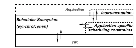
Fig. 1 System architecture

2 Overall System Architecture

The overall system architecture we consider is depicted in Fig. 1. The application code isinstrumentedso as to be able toobserve and control it. The instrumentation code keeps track of the state of the application and intercepts applica-tion requests for lower level mechanisms of interest for the scheduler (e.g., synchronisation, communication). The in-tercepted requests are redirected to a subsystem which is responsible for controlling the system. Thisscheduler sub-system uses a number ofscheduler constraints, which are application specific, to make a decision. These decisions are about whether it should block the application requests, when they may lead to an unsafe (or suboptimal) system state, or forward them to the underlyingOS. Finally, theOS primi-tives are effectively our means toobserve and interactwith the environment and the application.

This is a general system architecture for reactive sys-tems and closed-loop control. In the RMA/PCP framework, the “instrumented” synchronisation, etc. primitives use a set of scheduler constraints that together form the RMA/PCP priorities. In our context, the dynamic, application-specific scheduling constraints are automatically synthesised from a stopwatch automata model of the application and its envi-ronment.

The primitives of interest for control are the synchro-nisation by means of monitors (monitorEnter, monitor-Exit) and the communication by means of condition

vari-ables through notification, broadcasting, waiting for a notifi-cation and waiting for a notifinotifi-cation until some timeout ( no-tify,notifyAll,wait,timed wait), with the well-known POSIX[23] or Java [25] semantics. Finally, with waitFor-Periodperiodic application tasks wait for the arrival of their next period.

2.1 Scheduler Architecture

The architecture of theapplication-specific scheduling con-straintsthemselves is depicted in Fig. 2. As shown there, the application tasks make some request that is forwarded to one of two scheduler stacks. The left scheduler stack is responsible for electing some application task for execution, whereas the right stack elects a task as a target for a pending signal/notification. Both of these stacks have the same struc-ture; they are effectively subdivided into three main

lay-Safe−Exec

Quality−Notif Safe−Notif Ready−Notif

Quality−Exec Ready−Exec

SAFE TASKS SAFE TARGETS

TASKS READY

TO EXECUTE TASKS READY TOBE NOTIFIED

Blocked for I/O, etc. Mutual Exclusion Rules,

Condition Var. Notification Rules

CANDIDATES FOR

EXECUTION CANDIDATES FORNOTIFICATIONS

Application Application Tasks

Scheduler Scheduler Scheduler

Scheduler Scheduler

Scheduler

Increase System Quality

TASKS TO WAKE UP EXECUTING TASKS

OS

Execution Scheduler Stack Notification Scheduler Stack

Avoid Deadlocks Guarantee Deadlines

Increase System Quality

Avoid Deadlocks Guarantee Deadlines

Provide low−level mechanisms Sexec⊆ Rexec

Cexec Cnotif

Snotif ⊆ Rnotif

Rexec⊆ Cexec Rnotif ⊆ Cnotif

Choose one amongQexecfor execution Notify tasks inQnotif

Qexec⊆ Sexec Qnotif ⊆ Snotif

Fig. 2 Scheduler architecture

ers. The topmost scheduler layers (Ready-Exec, resp. Ready-Notif) identify application tasks which are eligible either for execution (Rexec) or for notification (Rnotif). They

effec-tively model in user-space the ready queue of the OSand its waiting-for-notification object queues respectively. The middle layers (Safe-Exec, resp.Safe-Notif) are the most im-portant in a critical system. They elect among the eligible tasks those that will not lead the system to a bad state (task

setsSexecandSnotif respectively). That is, the middle layers

are responsible for guaranteeing thesafetyproperties of the system (e.g., deadlock-freedom, meeting deadlines). Finally, the lower layers (Quality-Exec, resp.Quality-Notif) are re-sponsible for imposing further constraints, which are needed for guaranteeing other QoS system requirements, e.g., jitter minimisation, energy consumption minimisation, etc. The sets of safe tasks meeting these further quality constraints (Qexec, resp.Qnotif) form the final output of the application

dependent scheduler constraints subsystem. The scheduler subsystem passes them to theOS, which chooses tasks for execution, resp. notification, using someOSdependent rule. From the point of view of the scheduler, theOS choice is non-deterministic. It is exactly this non-determinism that al-lows designers to easily explore further scheduling strategies for the extra QoS requirements.

that is still occupied by the notifier. However, the left stack needs to be given control after notifications when scheduling for deadlines and other QoS, so as to ensure some hard to meet deadline/constraint by preempting the notifying task.

2.1.1 Increasing System Quality

As aforementioned, the bottomQuality-Exec and Quality-Notif layers of the scheduler, allow designers to easily ex-periment with and introduce additional constraints for in-creasing the quality of the system. Software engineers con-trol the complexity of these layers directly and can employ abest-effortpolicy or a more contract-like QoS one, where specific bounds for certain values of the system state must be guaranteed. In the latter case, the QoS policy must be ver-ified as a safety policy, to ensure that the system will never break its QoS contract.

A simple example of a (best-effort) quality policy is the local minimisation of context switches(LMCS), in order to speed-up the execution and (hopefully) minimise cache miss-es/flushes and, thus, also energy consumption. This policy can be implemented quite easily, by examining whether the currently executing task,ti, is in the setSexecof tasks which

are safe to execute next. If this is the case, then we can let it continue its execution, by setting the setQexec equal to

the singleton {ti}. Note, that LMCS differs from a

non-preemptive platform execution policy, since LMCS allows preemption when the currently executing task is not in the safe set.

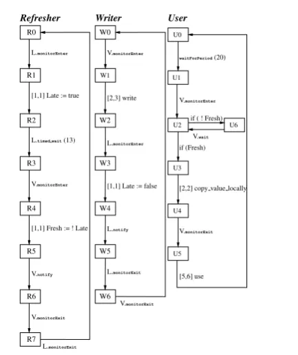
3 A Simple System

This section introduces the simple system of Fig. 3, to be used for illustrating the various notions through concrete ex-amples. The system consists of the Writer, User and Re-fresher tasks. The Writer produces values for variable V continuously (e.g., by reading a sensor or retrieving a stock price), which the periodic task User consumes. However, User needs the values of V to be fresh, i.e., they must have been produced recently and as such represent the current state of the environment. For that, the Refresher task uses an auxiliary variable L, to distinguish values of V that are too old, from these that are fresh enough for User. It does so by marking the current value of V as not fresh and then doing a timed wait for 13 time units. If the Writer produces a new value for V during that time, the freshness of V will be true, otherwise it will be false.

There is a potential deadlock between Writer and Re-fresher, as they obtain V and L in the opposite order, which arises when the Writer is at state W2 and the Refresher at state R3.

Refresher Writer User

U0

U1

U2 U6

U3

U4

U5 W1

W0

W2

W3 R0

W6 R1

W4 R2

W5 R3

R4

R6 R5

R7

L.monitorEnter

V.wait

[1,1] Fresh := ! Late

if ( ! Fresh)

L.notify

L.monitorExit [2,3] write

L.monitorEnter

[1,1] Late := false V.monitorEnter

L.timed wait(13) [1,1] Late := true

V.notify

V.monitorExit

waitForPeriod(20)

V.monitorEnter

if (Fresh)

[2,2] copy value locally

V.monitorExit

[5,6] use

L.monitorExit V.monitorExit

V.monitorEnter

Fig. 3 A simple three-task system

(Clock variables are omitted for readability – each computation is annotated with its duration interval. )

4 System Modelling

This section presents our modelling of a system through discrete-time stopwatch automata. Stopwatch automata al-low for fine grain modelling, thus permitting us to synthesise a flow-sensitive and not over-constraining scheduler, which needs fewer resources to meet requirements. The discrete-time stopwatch automata we are using are normal finite-state automata, where certain variables serve asdiscrete time clocks. The difference between the stopwatch automata we use and the (discrete) timed automata of [2, 20, 3] is that we can stop certain clocks (without resetting them) and restart them later on. Thus, we can easily model preemption. The difference with stopwatch automata [32, 26, 11] is that our clocks take discrete and not continuous values. As a conse-quence, reachability is decidable for discrete-time stopwatch automata, while it is not in general for continuous-time [26, 19].

4.1 Application Modelling

As aforementioned, we consider that the application com-prises a set of concurrently executing asynchronous tasks, T = {ti}i∈I, whereI is the set of task indexes. Tasks can

synchronise through monitors, communicate through condi-tion variables, wait for their next period or perform a com-putation.

R2 R2_Relock R1

R1 R2

R3 R3

L.receiveNotif L.timed wait(13)

L.monitorEnter [1,1] Late := true [1,1] Late := true

∨Timeout ; L.monitorExit

Fig. 4 Modelling of thewaitprimitive

must enter the monitor ofr(r.monitorEnter), notify tasks interested in events about this resource (r.notify/All) and subsequently leave the monitor (r.monitorExit). Tasks

in-terested on events for resource r, must enter its monitor, wait for an event (r.wait/timed wait), treat the event in an application specific manner and then leave the monitor. Note thatwaitprimitives force waiting tasks out of the cor-responding monitor, so as to allow notifying tasks to en-ter it. So,wait primitives are modelled by two states (R2, R2 Relock), as Fig. 4 shows using part of the Refresher’s model from Fig. 3. The transition from the previous state to the first one (R1→R2) makes the task leave the monitor, af-ter having executed the action the program was performing there ([1,1] Late := true). The transition from the first to the second wait states (R2→R2 Relock) waits for a notification (or a timeout if it is atimed wait). Once a task

is notified, it attempts to fire the transition from the second wait state to the subsequent program state (R2 Relock→ R3), so as to reenter the monitor and continue its execution. Each task uses two clocks to model time-related behaviour. The first clock,SWi, models the duration of computations

of taskti and so is stoppedwhen the computation is pre-empted.SWi is also used when a task performs atimed -wait, to measure the distance till the timeout. The second clock,C_iPeriodic, measures the time remaining until the next period (or deadline) of a task andis never stopped; it is only resetat each new period.

4.2 System State

The system state model comprises:(i)anabstractprogram counter (PCi) for each of the application tasks;(ii)a

stop-watch (SWi) for each task;(iii)Nperiodic clocks (CiPeriodic),

for theNperiodic tasks, taking values over the interval[0, Pi),

wherePiis the period of the task;(iv)N Boolean variables (taskAlarm), for dissociating the cases “start of period” and “deadline/end of period”, since for some tasks we may have Di = Pi (see section 7); (v)a variable (TExec) for

the currently executing task or IDLE when no task is ex-ecuting;(vi)a 4-valued variable (mode) controlling which of theSchedExec,SchedNotif,Timeout, or one of theApplicationautomata should execute in the current step (these automata are described in the following section); and(vii)theBooleanvariables of the application guarding waiting statements and branches, if we wish to model them.

mode =

Timeout

Application

mode =

Application

Schedulers Only

mode∈ {SchedExec,SchedNotif}

Timeout

New tick, check timeouts

No Timeouts, let Application run

Re-Schedule T

imeout(s) fired Check

timeouts

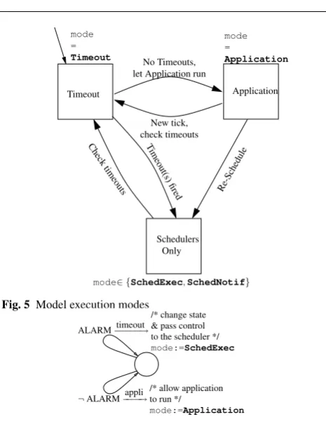
Fig. 5 Model execution modes

ALARM−−−−−→timeout

/* change state & pass control to the scheduler */ mode:=SchedExec

¬ALARM−appli−−−→

/* allow application to run */

mode:=Application

Fig. 6 Timeout automaton

Example 1 For the system of Fig. 3, the variables are: PCWriter∈ {W0,W1,W2,W3,W4,W5,W6},

PCRefresher∈ {R0,R1,R2,R3,R2 Relock,R4,R5,R6,R7}, PCUser∈ {U0,U1,U2,U3,U6,U4,U5,U6 Relock},

SWWriter∈[0,6],SWRefresher∈[0,13],

SWUser∈[0,6],CUserPeriodic∈[0,19],

User Alarm∈ {false,true},TExec∈ {IDLE,Writer,Refresher,User}, mode∈ {Sched-Exec/Notif,Timeout,Application},

Late∈ {false,true}, Fresh∈ {false,true} _N

4.3 Model Structure and Execution Modes

The system model we construct is the parallel composition of:

– TheTimeoutautomaton which fires timeouts,

– theExecutionandNotificationScheduler automata, and – one automaton for each of the application tasks.

Application automata are derived fromcontrol-flow diagrams describing the application tasks. These are annotated with the timing constraints modelling the execution times of the corresponding code. These models can also be extracted au-tomatically from application code, as was done in [28] and in [5] for annotated Java and C programs, respectively.

W

i ti∈ Rexec∩ Sexec∩ Qexec

Chooseti

−−−−−−−→TExec:=ti

Fig. 7 Execution Scheduler automaton

more timeouts (corresponding to a timed wait or wait-ForPeriod expiring) if any is enabled currently. When a timeout is fired, mode changes to “Schedulers Only” (where

mode = SchedExec), so that our scheduler can handle it. If there is no timeout to be fired then the mode changes to “Application” (wheremode=Application). At this mode, the automaton of theTExecapplication task becomes

enabled. If theTExectask needs to execute a time guarded

action (i.e., a computation), then it causes time to advance by performing a tick (i.e., a time step). The tick action causes all periodic clocks (C_iPeriodic) to advance at the same time. It also causes local stopwatches (SWi) to advance, if the

re-spective task is executing, i.e.,TExec=ti, or if it is

perform-ing atimed wait. Ticks change mode back toTimeout, so as to check for new timeouts. If, however,TExecneeds to

perform an action which causes re-scheduling, then it passes control back to the schedulers, i.e., mode becomes “Sched-ulers Only” (mode∈ {SchedExec,SchedNotif}). Ini-tiallymodeisTimeout, for periodic tasks to start their first period.

5 Scheduler Synthesis

This is essentially a two player game. For each scheduler action (i.e., selection of an application task), there is a se-quence of actions of its adversaries (i.e., timeout and appli-cation automata), and so on. In this game, scheduler syn-thesis amounts to finding awinning strategyfor each state where it is the turn of the scheduler to act, if any such strat-egy exists indeed [4]. That is, whenever the scheduler is called to perform acontrollableaction, it must have a plan that informs it which futureuncontrollableactions of its ad-versaries it should render impossible, in order for the system to remain in a safe state. Thus, the scheduler synthesis prob-lem can briefly be stated as “for each control state, find the environment actions that must be rendered impossible for the system to always remain in a safe (optimal) state.” In our case, we have two layers which are needed for guaran-teeing safety - the top one (Ready-Exec&Ready-Notif) and the middle one (Safe-Exec&Safe-Notif).

5.1 Synthesis of the Ready Task Layer

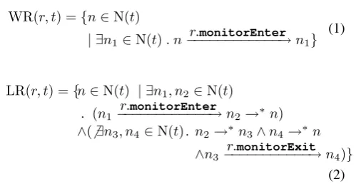
We synthesise the top layer through a simple static analy-sis of the task control-flow graphs. This assigns to each of the task states, N(t), the resources it holds and the ones

it wishes to lock, constructing two different sets for each task: one stating when task t wants to lock a resource r,

WR(r, t), and another one stating when the task has the re-source locked,LR(r, t):

WR(r, t) ={n∈N(t)

| ∃n1∈N(t). n

r.monitorEnter

−−−−−−−−−−−−→n1}

(1)

LR(r, t) ={n∈N(t) | ∃n1, n2∈N(t)

. (n1

r.monitorEnter

−−−−−−−−−−−−→n2→∗n)

∧(6 ∃n3, n4∈N(t). n2→∗n3∧n4→∗n

∧n3

r.monitorExit

−−−−−−−−−−−→n4)}

(2)

States with awaittransition are expanded as in Fig. 4. For theWRandLRsets, these are equivalent to a monitor-Exitand then amonitorEnteron the resource. Thei×j

sets produced, for theiprogram counters andj resources, inform us whether a task is blocked or not, which is needed for the topReady-ExecandReady-Notif scheduler layers.

Example 2 For the system of Fig. 3, these sets are: WR(V,Writer) :={W0},WR(L,Writer) :={W2},

LR(V,Writer) :={W1, W2, W3, W4, W5, W6},

LR(L,Writer) :={W3, W4, W5},

WR(V,Refresher) :={R3},

WR(L,Refresher) :={R0, R2Relock},

LR(V,Refresher) :={R4, R5, R6},

LR(L,Refresher) :={R1, R3, R4, R5, R6, R7},

WR(V,User) :={U1, U6Relock},

LR(V,User) :={U2, U3, U4},WR(L,User) := LR(V,User) :=∅ Potentialdeadlocks are easily identified by considering the intersection of the setsWRandLR. Indeed, there is a po-tentialdeadlock at states (W2,R3,*) because we have that:

WR(L,Writer)∩LR(V,Writer) ={W2}and

WR(V,Refresher)∩LR(L,Refresher) ={R3}_N

Of course one cannot be certain thatpotentialdeadlock states identified through theWRandLRsets arereal, until they are shown to bereachable. Attempting to render them unreachable by enclosing the corresponding critical regions inside a new monitor (e.g., enclose each ofR1-R7andW0

-W6 inside a monitor on a new resourceD) will certainly remove any chance forthat deadlock but will unnecessar-ily decrease the degree of concurrency in the system, es-pecially so if the deadlock is unreachable. In fact, for the system of Fig. 3, such a solution iswrong. Indeed, variable Fresh will never become true and User willneverfinish its period (states U3, U4, and U5 are unreachable). The rea-son for this is that wheneverRefresher gains access toD, it will set Fresh to false and remain in the monitor of D

or a web server dropping all client requests. Thus, we can see that this solution, advocated in [43] for its simplicity, can break the application logic itself by removing too many valid execution traces.

Nevertheless, setsWRandLRshow which are the tasks that cannot be involved in a deadlock, e.g., here the User task.

5.2 Synthesis of the Safe Task Layer

The basic method for synthesising theSafe-Execand Safe-Notif scheduler layer, starts by first constructing the set of reachable states and, thus, identifying the bad states. These are the states where the application tasks are deadlocked, or the states where some task has missed its deadline.

Having bad states means that the current setSexec, of

tasks that are safe to execute at a states, needs to be con-strained. The onlycontrollableactions that can be constrained in the system are the transitions of the scheduler automata, shown in Fig. 7.Sexec is initiallytrue, thus accepting all

tasks in the setRexecas safe. Having obtained the bad states,

we do a backwards traversal of the state space starting from the bad states, until we reach a state,s, which corresponds to a controllablechoice of one of the scheduler automata. There, we identify the controllable transitionaoutgoing from

s which setsTExec to be task ta, effectively enabling the

path leading to a bad state, and create a new constraint for the layerSafe-Execat statesfor the controllable transition

a. The constraint is constructed by changing the setSexecto

be:

S0

exec(s) :=Sexec(s)\ {ta} (3)

If at some point we find thatS0

exec(s)becomes equal to the

empty set after constraining it, that is, if there is no safe task to execute at states, then we also mark the statesas bad and continue the synthesis procedure.

So, the set of states where a tasktis unsafe to execute is:

Unsafe(t) ={s|t∈ Rexec(s)∧ ¬Sexec(s)} (4)

Example 3 This set is expressed as a predicate over model variables. Table 1(a) shows the synthesised predicateUnsafe( Refresher)for ensuring the timeliness property ofUser(i.e., its period is never violated). The constraints essentially for-bid Refresher from executing when User is about to miss its deadline (e.g., atU1∧CPeriodic

User = 11), since Refresher

would consume computational resources and/or invalidate the current value of V, in which case the User would need to wait for a new fresh value to be produced._N

5.2.1 Partial State Observability

In reality, the scheduler cannot observe the full state of the system. That is, the scheduler uses an observation function,

obs, presenting it with a partial view of the current system state. Our default assumption is that the scheduler sees at most the values of the task program counters,PCi, and those

of the clocks, i.e.,SWiandCiPeriodic, along with the value

of the last task that was executing,TExec. All other system

variables are hidden to it. The scheduler can observe these variables only, so that the instrumentation of the application will be minimal and easy to perform in practice, though sys-tem designers are free to enlarge the observation set. So the scheduler synthesis procedure really uses (5) and (6), rather than(3) and(4):

S_exec0 (obs(s)) :=Sexec(obs(s))\ {ta} (5)

Unsafe(t) ={s|t∈ Rexec(obs(s))∧ ¬Sexec(obs(s))} (6)

Example 4 Again for the system of Fig. 3, the constraints we synthesise to render the system deadlock-free, once we have applied the projection on the state variables are:

Unsafe(User) := FALSE(i.e., always safe)

Unsafe(Writer) := (PCWriter = W0)∧(PCRefresher =

R3)

Unsafe(Refresher) := (PCRefresher=R2 Relock)

∧(PCWriter∈ {W1, W2})

Table 1(b) shows timeliness constraints for Refresher, when hiding clocks._N

A consequence of the partial state observability is that the synthesised scheduler is not necessarily themaximalone. This is because the scheduler may apply more constraints than is absolutely required to some system states, if these constraints are needed by states that are equal tosmodulo the observation function.

5.2.2 Branching Bisimulation Equivalence Reduction

Table 1 Refresher timeliness constraints

(a) Refresher constraints when observing clocks and allowing preemption

LET A = (PCUser=U5 ∧ C_UserPeriodic=13)

IN (A ∧ (PCRefresher=R0 ∧ (PCWriter=W0)

∨ (PCWriter=W2 ∧ ((TExec=PCRefresher ∨ TExec=PCWriter)))

∨ (PCWriter=W6 ∧ TExec=PCWriter))

∨ (PCRefresher=R3 ∧ PCWriter=W0)

(b) Refresher constraints when not observing clocks

(PCRefresher=R7 ∧ PCUser=U1 ∧ PCWriter=W1 ∧ TExec=PCWriter)

The synthesised scheduler for thebbe-reduced system will be exactly the same with the one we would have synthe-sised for the non-reduced system. This is because in our ini-tial parallel automata model, it is always the case that either some state has outgoingτ transitions or transitions labelled by some non-τ scheduler actiona. Indeed, note that when the mode variable equals SchedExec or SchedNotif

the current state has only non-τ transitions enabled (those of the scheduler automata), while in modesTimeoutand

Applicationwe can only performτtransitions. So, it is neverthe case that a state,s, can do both aτand ana transi-tion, wherea6=τ. As a consequence, after thebbereduction on the initial state space graph, we obtain classes of equiva-lence, where,if we can leave them with a transitiona, then we cannot leave them with a transition τ and vice versa. So, the controllable equivalence classes are characterised by their frontier, which is exactly the member states hav-ing non-τtransitions. So, we define the frontier of a class,c, ofbbe-equivalent states as in (7), whereenable()produces the set of states enabling a particular transition. Note that the frontier of an uncontrollable equivalence class is the empty set,∅:

frontier(c) =c∩ \

a6=τ

enable(a) (7)

5.2.3 Synthesis Procedure

The synthesis procedure has three steps. First, the bbe re-duction is applied. Then, scheduling constraints are synthe-sised. This assigns to each branching bisimilar classcthe set

Bad(c), i.e., the transitions the scheduler must not take in that class for the system to stay safe. If aτaction is a mem-ber ofBad(c)then the whole classcis marked as unsafe. Otherwise, the constraints of c are assigned to its control-lable member states, i.e., the states incthat have at least one non-τtransition. This effectively computes the setSexec. So,

for alls∈frontier(c), whereBad(s) = Bad(c):

S_exec0 (s) :=Sexec(s)\ {ta|a∈Bad(s)} (8)

When using the observation functionobsto project the states of the frontier to the observable system variables, we may cause classes to share projected states, i.e., there may be

two classes, say candc0, such that obs(s) = obs(s0)for somes∈frontier(c)ands0∈frontier(c0), or, equivalently:

obs(frontier(c))∩obs(frontier(c0))6=∅.

This means that the scheduler cannot dissociate these states, so eachprojected frontierstate is assigned theunionof all the constraints of thebbe-equivalent classes it is a member of:

Sexec0 (obs(s)) :=Sexec(obs(s))\ {ta|a∈Bad(obs(s))(9)

Bad(obs(s)) = Bad({c|obs(s)∈obs(frontier(c))})(10)

6 A Methodology for Synthesis

Despite thebbe reduction, the size of the state space can still be considerable. Therefore, it is imperative that synthe-sis follows a methodology which reduces the state-space ex-plosion problem. Another problem with scheduler synthesis is that the resulting scheduling constraints can be difficult to understand and relate to specific system properties.

Thus, the methodology for scheduler synthesis presented herein has a dualpurpose. First, it reduces the size of the state space, by synthesising schedulers for successively more detailed models. In this way, more complex models are only considered when a safe scheduler has been synthesised al-ready for a more constrained version of the model. Second, this methodology also has as a purpose (and advantage) to synthesise scheduler constraints that are more easily related to a specific safety property and platform execution model. So, it can be immediately identified which constraints are needed for avoiding deadlocks due to resource synchronisa-tion, which ones for meeting deadlines when computations are not preemptable, etc. Thus, it is easier to understand the constraints themselves, as well as, the behaviour of the dif-ferent system tasks and their importance as far as each safety property is concerned, leading to a better analysis of the sys-tem under scrutiny. This is advantageous both for validating the synthesised scheduling constraints and for discovering ways to optimise the system further [27].

We take advantage of these aspects by performing scheduler synthesis in four major steps.

6.1 Abstraction of Time

First, we consider the issue oftime, by examining the un-timed model of the system and synthesising a scheduler to guarantee theabsence of deadlocksdue to synchronisation. For the case study of section 7, the reduction obtained is 97% of the full timed model (see line(2)of Table 3).

Example 5 Indeed, for the example of Fig. 3, the synthe-sised constraints on the untimed model remove the dead-locks due to the wrong synchronisation of Writer and Re-fresher.

While the system cannot deadlock anymore, there are still cases where User misses its period. Bad states repre-senting these timeliness violations must be rendered unreach-able through further constraints. Tunreach-able 2 shows the results from the various synthesis stages for achieving this (lines(3), (5)and(7)), by synthesising 163 additional constraints.N

Finding and removingalldeadlocks in the untimed model means that the synchronisation protocols used arelogically correct. That is, no deadlocks will ever occur, even if com-putation execution times have been wrongly estimated or they change later on, by changing implementations, port-ing to different hardware platforms, usport-ing more processors, etc. This is particularly important for product families, since there the timing information differs for each family mem-ber [13].

Having found all the deadlocks in the untimed system, we impose the synthesisedSexec andSnotif scheduler

con-straints upon thetimedmodel, and search fortimeliness con-straints, so that all tasks will meet their deadlines.

6.2 Platform Execution Model

Again, we do not attack the full timed model immediately but consider first a constrained version of it, where tasks execute under anon-preemptiveexecution model. The non-preemptive platform execution model reduces the state space by removing all cases where an interrupt suspends a task computation.

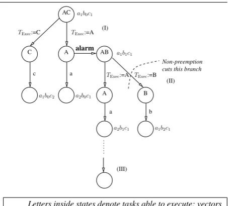
6.2.1 Non-Preemption and Scheduler Synthesis

To better explain the benefits of examining the non-preemptive execution model first, let us consider the example in Fig. 8. As shown there, when imposing the non-preemptive execu-tion model at state AB we are effectively cutting the branch AB →B, where the scheduler chose to preempt the exe-cution of task A with task B after the alarm. This kind of

Non-preemption

(III) a1b0c1

AC

TExec:=A

a c

a1b1c1

TExec:=A TExec:=B

a b

..

..

..

cuts this branch (I)

(II)

C A AB

A B

TExec:=C

a2b0c1

a1b2c1

a2b1c1

a1b0c2

alarm

Letters inside states denote tasks able to execute; vectors beside the states show possible values of the taskPCs.

Fig. 8 Preemption and state space size

reduction has a repercussion on the preemptive execution model we will examine subsequently. The result of exam-ining the non-preemptive case first, depends on the kind of scheduler we will synthesise. If in the non-preemptive case we find that there is a winning strategy at point (III) and so we do not forbid branch AB→A, then adding preemp-tion at the next stage will simply add branch AB→B. If, however, branch AB→A in the non-preemptive model is unsafe, then we will be obliged to constrain the system ear-lier on (since now branch AB→B is not available). If we needed to constrain the system at state AC, by cutting branch AC→A and selecting branch AC→C, then permitting pre-emption later on would mean that the whole sub-graph after branch AC→A will have been removed by the scheduler we synthesised for the non-preemptive execution model. There-fore, we have gained by being able to examine the inherent non-determinism of the scheduler synthesis problem, with-out being overwhelmed by the additional non-determinism introduced by the interrupts.

Once we can safely schedule the system for a non-preemptive execution model, we use the scheduling constraints to re-duce even furtherthe state space that we have to analyse, when we permit preemption. Observed reductions with the non-preemptive execution model and thebbereduction ranged around 95% of the preemptive, unconstrained timed model (see lines(3)and(11)of Table 3).

The non-preemption of tasks is easily added to our mod-elsthrough the use of a quality-level policythat forbids the schedulers from choosing a task for execution, when another task is already in a state where it is computing:

Qexec(obs(s)) :={t|computes(t) (11)

Example 6 For the system of Fig. 3, thebbe-reduced non-preemptive system has 973 states (see line(3)of Table 2), while thebbe-reduced preemptive one has 804 states (using the constraints from the non-preemptive one, line(5))._N

It is still worthwhile to perform these separate synthesis steps even when the gains in state reduction are not spec-tacular, since it helps to understand the system behaviour better.

We should note here that we cannot safely schedule all systems when we do not allow tasks to be preempted. In-deed, in eq. (11) we explicitly ignore the set of safe tasks (Sexec) when some task is computing. For these systems we

will not obtain any scheduling constraints and, therefore, will be obliged to examine the larger, unconstrained state space of the timed model, corresponding to a preemptive execution model.

6.3 Policies for Overall System Quality

Once we have synthesised a safe scheduler for deadlocks and deadlines, we can compose it with other policies to fur-ther constrain the set of safe states to those guaranteeing other QoS system requirements, e.g., memory or energy con-sumption, jitter minimisation, etc. Designers can balance be-tween the execution time and extra memory needed by these policies and the gains they offer to the overall system qual-ity.

The aforementioned LMCS policy observes only the cur-rent system state, while more complex policies may examine application variables or the execution history. Such a policy, which also observes an application variable, is the optimisa-tion policy of eq (12), which favoursUserto proceed if the current value is fresh. Multiple QoS policies can be applied as is shown in lines(13)–(14)of Table 2, where the policy of eq. (12) has been applied to the safe system of line(8)and then the LMCS policy has been applied on top of it.

TExec:= 

    

    

{User} whenPCUser=U1∧PCWriter=W0

∧User∈ Sexec∧Fresh =true

{Writer}whenPCUser=U1∧PCWriter=W0

∧Writer∈ Sexec∧Fresh =false

TExec otherwise

(12)

6.4 Compositional Synthesis

Finally, designers can partition the system and independently synthesise constraints for subsystems. Then the synthesis al-gorithm is applied again on the parallel composition of the

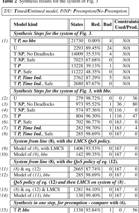
Table 2 Synthesis results for the system of Fig. 3

T/U:Timed/Untimed model, P/NP:Preemption/No-Preemption

Model kind States Red. Bad Constraints

Used/Prod.

Synthesis Steps for the system of Fig. 3.

(1) TP, no bbe 21730 0.00% 4 N/A

U 2293 89.45% 24 N/A

TNP, No Deadlocks 14009 35.53% 4 N/A

TNP, Safe 7023 67.68% 0 N/A

TP 13228 39.13% 1 N/A

TP, Safe 11222 48.35% 0 N/A

TP, Time Ind. 2762 87.29% 5 N/A

TP, Time Ind., Safe 2680 87.67% 0 N/A

Synthesis Steps for the system of Fig. 3, with bbe.

(2) U 279 98.72% 0 0/ 36

(3) TNP, No Deadlocks 973 95.52% 1 36/ 80

(4) TNP, Safe 574 97.36% 0 116/ 0

(5) TP 804 96.30% 1 116/ 47

(6) TP, Safe 702 96.77% 0 163/ 0

(7) TP, Time Ind. 282 98.70% 1 163/ 4

(8) TP, Time Ind., Safe 285 98.69% 0 167/ 0

System from line(8), with the LMCS QoS policy.

(9) Model of(8), with LMCS 1406 93.53% 0 167/ 0

(10) Model of(9),bbe 142 99.35% 0 167/ 0

System from line(8), with the QoS policy of eq.(12).

(11) (8)& eq. (12) 2665 87.74% 0 167/ 0

(12) Model of(11),bbe 285 98.69% 0 167/ 0

QoS policy of eq.(12)and then LMCS on system of (8) .

(13) (8)& eq. (12) & LMCS 1281 94.10% 0 167/ 0

(14) Model of(13),bbe 130 99.40% 0 167/ 0

Synthesis in one step, for preemption - compare with (6).

(15) TP, bbe 1338 93.84% 1 0/ 56

already constrained models, to obtain a scheduler guarantee-ing the safety properties for the whole system.

Such a compositional synthesis allows designers to anal-yse bigger systems. Sometimes even ignoring a single task can make a great difference in the resulting state space - in our case study we observed a reduction of 82% by doing so (from 353730 down to 62137 states), see section 7.

Example 7 Table 2 shows the results of our methodology for the system of Fig. 3. As shown in line(15), without our methodology, one has to attack the full state space, which contains 21730 states (1338 after the bbereduction), and will synthesise 56 constraints, instead of 167._N

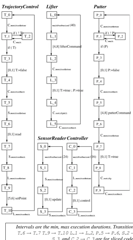
Controller Lifter

TrajectoryControl Putter

SensorReader

P_0

P_3

P_1 P_2

P_4

P_5

P_6

P_8

P_9 P_7

S_2 C_2

S_0 C_0

C_1 S_1

C_3 S_3

T_1

T_8 T_0

T_3

T_2

T_4

L_0

T_7

T_10

L_1

T_5

L_2

T_9 T_6

L_3

L_4

L_5 C.notifyAll

[0,1] T:=true ; P:=true C.monitorEnter

[4,8] lifterCommand

waitForPeriod(40)

C.monitorExit

[0,1] update S.monitorEnter waitForPeriod(24)

S.monitorExit

[0,1] control L.monitorEnter waitForPeriod(16)

L.monitorExit

C.monitorEnter

[0,1] T:=false

C.monitorExit

S.monitorEnter

[0,1] read

S.monitorExit

L.monitorEnter

[5,6] setPoint if ( T)

L.monitorExit

if ( ! T)

C.wait

C.notify

[0,1] T:=true C.monitorEnter

[4,8] putterCommand C.monitorExit

[0,1] P:=false if (P) C.monitorEnter

C.monitorExit

if ( ! P)

C.wait

Intervals are the min, max execution durations. Transitions T 6→T 7 T 9→T 10 L 1→L 2,P 5→P 6,S 2→ S 3, andC 2→C 3are for sliced code.

Fig. 9 Control-flow graphs of the tasks of a robotic arm

7 Case Study: A Robotic Arm

In this section we consider a case study based on a robotic arm system from [42], shown in Fig. 9. The arm takes ob-jects from a conveyor belt, stores them temporarily in a buffer shelf, and puts them into a basket. The arm is controlled by tasks running on a single processor.

Fig. 9 shows the control-flow graphs of the tasks.

Tra-jectoryControlreads commands from a shared buffer

(C) and issues set-points (L) to the low-level arm Control-ler. If there are no commands (modelled by the predicate

T) it holds, otherwise it reads the sensor value (S) and com-putes a new set-point. Its execution time is between 5ms and 8ms. There are two motion executors,LifterandPutter.

Lifteris activated periodically every 40ms. It commands the arm to pick objects from the belt and place them into the buffer shelf. Upon termination, it issues a command to

TrajectoryControland activatesPutter, sending it

commands for moving the object from the shelf to the

bas-ket (predicateP). Its execution time is between 4ms to 9ms.

Puttersends commands to move the object from the shelf into the basket. Its execution time is between 4ms to 10ms.

The SensorReader task reads sensors every 24ms. Its

execution time is 1ms. Sensor readings are used by

Tra-jectoryControl.Controlleris a periodic task with

a period of 16ms.

L5

mode =Appl.∧TExec= Lifter∧SWLifter<1

⇒ Advance Running Clocks ; mode :=Timeout

mode =Appl.∧TExec= Lifter∧SWLifter<8

⇒Advance Running Clocks ; mode :=Timeout

mode =Appl.∧TExec= Lifter⇒C.monitorEnter

mode =Appl.∧TExec= Lifter⇒C.notifyAll

mode =Appl.∧TExec= Lifter∧SWLifter≥4∧SWLifter≤8

⇒ /* ask permission for locking C */ SWLifter:= 0 ; mode :=SchedExec

mode =Appl.∧TExec= Lifter∧SWLifter≥0∧SWLifter≤1

⇒ /* ask permission for notifying */ T := true ; P := true ;SWLifter:= 0 ; mode :=SchedNotif

(Synchronised with the transition T0−α→T0

of the Timeout automaton, see Fig. 11)

mode =Appl.∧TExec= Lifter

⇒ /* ask permission for continuing */ C.monitorExit; mode :=SchedExec

L0

L1

L2

L3

L4

mode =Appl.∧TExec= Lifter∧CPeriodicLifter 6= 0

⇒Advance Running Clocks ; mode :=Timeout

Fig. 10 Lifter’s automaton

7.1 Stopwatch Automata Model of the Robotic Arm

Fig. 10 showsLifter’s stopwatch automaton model. Note how the mode is changing - after each clock tick (e.g., L1

→L1), which increases all running clocks/stopwatches, the

mode changes toTimeout, so that we can check for deadli-nes/alarms. Mode changes toSchedExecbefore each mon-itorEnter(L1 →L2), to ask the Execution scheduler for

permission to enter the monitor. It also changes toSchedExec

aftereach monitorExit(L5 →L0), to get permission for

continuing execution. Note finally, that before performing thenotifyAllat state L4, mode changed toSchedNotif,

so that the Notification scheduler stack can decide what task(s), if any, should be notified.

Fig. 11 shows the part of the Timeout automaton which is relative toLifter. Transition T0

α

mode =Timeout ∧ ¬enabled(α) ∧ ¬enabled(β) ⇒mode :=Appl.

T1

Deadlock State mode =Timeout ∧CPeriodic

Lifter mod 40 = 0

∧Lifter Alarm∧Lifter = L0

⇒

Lifter := L1;SWLifter:= 0 ;

Lifter Alarm := false ; mode :=SchedExec

T0

α γ

δ

mode =Timeout ∧(CPeriodic

Lifter mod 40 = 0)

∧Lifter6=L0

∧Lifter Alarm⇒skip /* Don’t change mode

so as to deadlock */ β

mode =Appl. ∧TExec= IDLE

⇒

Advance Running Clocks ; mode :=Timeout; Lifter Alarm := true

Fig. 11 Timeout automaton (Lifter’s part)

which is a multiple of its period. In this case, mode changes toSchedExecso that the Execution scheduler can respond to this “new task period” event. Transition T0

γ

−→T0is used

when there is no deadline/period to be signalled; we simply change mode back toApplicationto allow the

applica-tion to continue. Transiapplica-tion T0−→δ T0is for the case where

the scheduler had selected the IDLE task to execute; we just advanceallrunning clocks/stopwatches (arming all alarms as a byproduct), waiting for a timeout. Finally, transition T0

β

−→T1is whenLiftermisses its deadline. In this case we

move to a deadlock state and do not change mode; thus now the whole system becomes deadlocked. The Boolean vari-able Lifter Alarm is used to dissociate between the cases

CPeriodic

Lifter = 0(start of period) andCLifterPeriodic = 40

(dead-line). In the former case Lifter Alarm is false and thus the deadlocking transitionβis disabled, while in the latter case Lifter Alarm is true and transitionβ is enabled. This vari-able starts with a value of true, gets disvari-abled at each new period andautomatically becomes enabled by each tick.

7.2 Applying Scheduler Synthesis

We decided to partition the application in two sub-systems, one comprising 4 tasks, namely,Lifter,Putter,

Sensor-Reader, andTrajectoryControl, and another one

con-sisting solely of theControllertask. Table 3 shows the results obtained when applying our methodology on the case study. We started with the untimed model of the 4-task sys-tem, so as to check for deadlock states (see line(2)of Ta-ble 3). Not finding any, we used a non-preemptive execu-tion policy to check the timed model of the system for states where deadlines are missed (line(3)). Such states indeed ex-ist and we synthesised 103 scheduler constraints for avoid-ing them. In line(4)we see that when applying these con-straints to the model, all deadline-miss states become un-reachable (always assuming a non-preemptive task execu-tion policy). Then, in line(5)we considered the timed model of the system under a preemptive execution policy. In this model, there are 15 more constraints we synthesise for avoid-ing the states where we can miss some deadline. When addavoid-ing these 15 constraints to our scheduler we obtain a safe

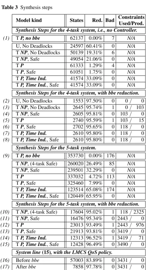
4-Table 3 Synthesis steps

Model kind States Red. Bad Constraints

Used/Prod.

Synthesis Steps for the 4-task system, i.e., no Controller.

(1) TP, no bbe 62137 0.00% 7 N/A

U, No Deadlocks 24597 60.41% 0 N/A

TNP, No Deadlocks 50139 19.31% 6 N/A

TNP, Safe 49054 21.06% 0 N/A

TP 61333 1.29% 4 N/A

TP, Safe 61051 1.75% 0 N/A

TP, Time Ind. 41574 33.09% 0 N/A

TP, Time Ind., Safe 41574 33.09% 0 N/A

Synthesis Steps for the 4-task system, with bbe reduction.

(2) U, No Deadlocks 1553 97.50% 0 0/ 0

(3) TNP, No Deadlocks 2645 95.74% 1 0/ 103

(4) TNP, Safe 2605 95.81% 0 103/ 0

(5) TP 2740 95.59% 1 103/ 15

(6) TP, Safe 2702 95.65% 0 118/ 0

(7) TP, Time Ind. 2610 95.80% 0 118/ 0

(8) TP, Time Ind., Safe 2610 95.80% 0 118/ 0

Synthesis Steps for the 5-task system.

(9) TP, no bbe 353730 0.00% 176 N/A

TNP, (4-task Safe) 260020 26.49% 85 N/A

TNP, Safe 239501 32.29% 0 N/A

TP 337032 4.72% 113 N/A

TP, Safe 325460 7.99% 0 N/A

TP, Time Ind. 123514 65.08% 174 N/A

TP, Time Ind., Safe 120449 65.95% 0 N/A

Synthesis Steps for the 5-task system, with bbe reduction.

(10) TNP, (4-task Safe) 17604 95.02% 1 118/2325

(11) TNP, Safe 16476 95.34% 0 2443/ 0

(12) TP 23013 93.49% 1 2443/ 976

(13) TP, Safe 21913 93.81% 0 3419/ 0

(14) TP, Time Ind. 12313 96.52% 1 3419/ 71

(15) TP, Time Ind., Safe 12428 96.49% 0 3490/ 0

System line(15), with the LMCS QoS policy.

(16) Beforebbe 57003 83.89% 0 3431/ 0

(17) Afterbbe 7858 97.78% 0 3431/ 0

task system, under both a non-preemptive and a preemp-tive execution policy, driven by a synthesised scheduler con-sisting of 118 constraints in total, as shown in line(6). In lines(7)and(8), we have attempted to synthesise constraints for the deadlines, when the scheduler is not allowed to ob-serve the clock values. As can be seen, no extra constraints are needed, meaning that the 118-constraint scheduler from line(5)is already independent of time when the clock valu-ations are projected out of the constraints.

all deadline-miss states have become unreachable. Then, in line(12), we examined the timed model under a preemptive execution policy, synthesising 976 new constraints. Using all the 3419 synthesised constraints, in line(13)we checked that they safely scheduled the system and then in line(14) we synthesised the final set of 71 constraints that are needed for a time-independent scheduler. The resulting scheduler (line (15)) has 3490 constraints, which keep the system in a safe state under both a non-preemptive and a preemptive execution policy, without observing the system clocks.

Finally, lines(16)and(17)apply the LMCS quality pol-icy to the system of line (15), whose effect is to halve the number of states of the safe system. This shows that the pre-emptive, time-independent scheduler synthesised at line(15) does not over-constrain the system, thus allowing designers to effectively attack further quality properties.

8 Scheduler Implementation

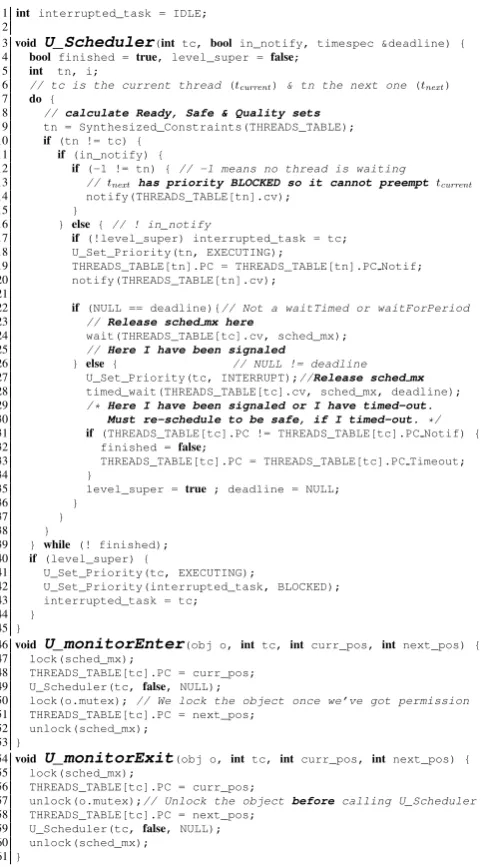
Once we have synthesised a scheduler we need to integrate it with the code of the application and the underlyingOS. Time-independent schedulers can be easily implemented us-ing widely available OSprimitives, i.e., a preemptive, pri-ority based FIFO scheduling policy, notify, notifyAll, waitandtimed waiton condition variables, and mutexes without priority inheritance. Time-dependent schedulers need in addition alarms and response time timers, if the dead-lines on the computations have been transformed to response times. Such timers are available in almost allOS’s. If, how-ever, deadlines refer toexecutiontimes, then we need timers capable of measuring the exact execution time of compu-tations, even in the presence of preemptions, which are not widely available. For exactly this reason, our methodology produces time-independent schedulers at the last stage - to avoid requiring extremely reliable and precise timers. In fact, we also developed a version of our control subsystem for supporting synthesised schedulers on FAST-OS, the propri-etary POSIX-compliantOSof Thal`es Airborne Systems, for the PowerPC architecture. Unlike mostOS’s, FAST-OS does not allow direct setting/observation of timers at all. In the following, we present the core implementation of time-independent schedulers.

The generated code consists of two parts - the appli-cation code and the control subsystem (U Scheduler). The application code is instrumented to callU Scheduler

when an application thread executes one ofmonitorEnter,

monitorExit,notify,notifyAll,wait,timed wait or

waitForPeriod. In its turn, U Schedulerevaluates the application-specific synthesised scheduling constraints cor-responding to the different scheduler layers. The control sub-system is implemented as an accompanying library.

Our library uses a single mutex (sched mx) and pro-vides to each application thread a unique condition variable.

1 int interrupted_task = IDLE; 2

3void U_Scheduler(int tc,bool in_notify, timespec &deadline) { 4 bool finished =true, level_super =false;

5 int tn, i;

6 // tc is the current thread(tcurrent) & tn the next one(tnext) 7 do {

8 //calculate Ready, Safe & Quality sets

9 tn = Synthesized_Constraints(THREADS_TABLE); 10 if(tn != tc) {

11 if (in_notify) {

12 if (-1 != tn) {// -1 means no thread is waiting 13 //tnext has priority BLOCKED so it cannot preempttcurrent 14 notify(THREADS_TABLE[tn].cv);

15 }

16 } else{ // ! in_notify

17 if (!level_super) interrupted_task = tc; 18 U_Set_Priority(tn, EXECUTING);

19 THREADS_TABLE[tn].PC = THREADS_TABLE[tn].PC Notif; 20 notify(THREADS_TABLE[tn].cv);

21

22 if (NULL == deadline){// Not a waitTimed or waitForPeriod

23 //Release sched mx here

24 wait(THREADS_TABLE[tc].cv, sched_mx);

25 //Here I have been signaled

26 } else{ // NULL != deadline

27 U_Set_Priority(tc, INTERRUPT);//Release sched mx

28 timed_wait(THREADS_TABLE[tc].cv, sched_mx, deadline);

29 /*Here I have been signaled or I have timed-out.

30 Must re-schedule to be safe, if I timed-out.*/

31 if(THREADS_TABLE[tc].PC != THREADS_TABLE[tc].PC Notif) { 32 finished = false;

33 THREADS_TABLE[tc].PC = THREADS_TABLE[tc].PC Timeout;

34 }

35 level_super =true; deadline = NULL;

36 }

37 }

38 }

39 } while(! finished);

40 if (level_super) {

41 U_Set_Priority(tc, EXECUTING);

42 U_Set_Priority(interrupted_task, BLOCKED); 43 interrupted_task = tc;

44 } 45}

46void U_monitorEnter(obj o, int tc,int curr_pos,int next_pos) { 47 lock(sched_mx);

48 THREADS_TABLE[tc].PC = curr_pos; 49 U_Scheduler(tc,false, NULL);

50 lock(o.mutex);// We lock the object once we’ve got permission 51 THREADS_TABLE[tc].PC = next_pos;

52 unlock(sched_mx); 53}

54void U_monitorExit(obj o,int tc,int curr_pos, intnext_pos) { 55 lock(sched_mx);

56 THREADS_TABLE[tc].PC = curr_pos;

57 unlock(o.mutex);// Unlock the objectbefore calling U_Scheduler 58 THREADS_TABLE[tc].PC = next_pos;

59 U_Scheduler(tc,false, NULL); 60 unlock(sched_mx);

61}

Fig. 12 Pseudo-code of the application scheduler

Table 4 Timing primitives undereCos(results inµs)

Primitive Min Avg. Max Avg.-Dev.

Synthesised Constraints 0.00 0.66 4.00 0.45

Context Switch 0.00 0.77 1.00 0.35

Trylock (unlocked) 0.00 0.69 2.00 0.47

Unlock (locked) 0.00 0.75 3.00 0.47

These condition variables are all associated with the afore-mentioned mutex (a capability which exists in POSIXbut not in Java). This construct is used simply for simulating the dis-abling of interrupts and can be used when our code needs to run in user space. Finally, we use three different priority lev-els, namely,BLOCKED,EXECUTING&INTERRUPT(from lowest to highest) and theSCHED FIFOPOSIXscheduling policy.

Fig. 12 shows the pseudo-code of the implementation.

and updates the application task’s position to be the same as in the model (lines 47–48).U SchedulercallsSynthesized -Constraints(generated by the synthesis tool) in line 9, passing it the current task PC’s. If the thread to be exe-cuted next (tnext) is different from the current one (tcurrent)

andtcurrentis not doing a notification,tnext’s priority is set

toEXECUTING(line 18), the condition variable (cvtnext) of

tnext is notified in line 20 and we finish by havingtcurrent

wait on its own condition variable,cvtcurrent, in line 24. This

final action releases sched mxjust before blocking, thus allowing the notified thread tnext to resume execution. If tnext is the same astcurrent, then the application scheduler

returns normally andtcurrentunlockssched mx.

The algorithm changes somewhat when calling the ap-plication scheduler through atimed waitor a waitForPe-riod. In this case, we also pass to our scheduler the time that the current thread should wait. The scheduler then performs a timed wait on cvtcurrent in line 28, using as timeout the

absolutedeadline argument, instead of doing a simple wait. It also increases the priority oftcurrent toINTERRUPTjust

before performing the timed wait (line 27), so thattcurrent

gets the CPU when it timeouts. Whentcurrent timeouts, it

re-evaluates the scheduler predicates (line 32), so as to find out if it is indeed safe to continue execution. Before calling

U Scheduler, functionsU timed wait/U wait(not shown

in Fig. 12) set fieldPC Notifto the label of to the internal state of the wait, where the thread has been notified but has not yet re-acquired the mutex of the object on which it was waiting. Similarly,functionsU timed wait/U wait for -periodset fieldPC Timeoutto the label of the internal state of the timed wait, or the label of the first statement after a new period.

We have successfully executed our implementation over two different combinations of hardware architecture and em-beddedOS’s, namely an Intel Pentium II (333MHz) running

eCosover Linux and a PowerPC simulator with FAST-OS. Experiments witheCosshowed that the execution time of the synthesised predicates (i.e., functionSynthesized -Constraints) is comparable to the execution time of lock-ing an (unlocked) mutex, havlock-ing a WCET in the order of 4µs. Table 4 gives the results of our experiments undereCos. Experiments were run 1000 times on a 330 MHz Pentium II, whereeCoswas using the synthetic Linux hardware archi-tecture, e.g., running over Linux as a user process.eCos

had the highest real-time priority in SCHED FIFO schedul-ing policy, thus runnschedul-ing uninterrupted byallother processes. In addition, all memory pages of the eCos process were locked in RAM, so as to avoid paging from theOS.

The implementation pseudo-code shown in Fig. 12 refers to a POSIX-API implementation of this library. This imple-mentation had to support FAST-OS that does not allow ac-cess to alarms. This is why timeouts (for Utimed wait/U wait-ForPeriod) were implemented with thetimed wait

primi-tive. We also have a non-POSIXimplementation overeCos

that usesOSalarms and alarm handlers directly, giving us finer control over timeout events, since these are now treated by high priority interrupt handlers. In this way we can sup-port deadline and period miss handlers as proposed by RTSJ [34].

9 Scheduler Robustness

Synthesised schedulers can be intolerable to wrong estima-tion of computaestima-tion WCET’s. In fact, a computaestima-tion should not finish earlier than its BCET either; in both cases the sys-tem enters a state that was not in the model used to synthe-sise the scheduler. Since this state was not explored during synthesis, the scheduler does not have a strategy for it and thus can take an unsafe action. It should be noted that by un-safe we mean to an action leading to a deadline miss, since deadlocks have been eliminated using the untimed model of the system, thus the deadlock-safety synthesised constraints are not sensitive to timing errors (indeed, our scheduler syn-thesis methodology is explicitly meant to guard against such a situation).

The simplest solution for BCET is toimposeit for each computation, by idling. This, however, implies that we ei-ther use a non-preemptive execution model, or that we have execution time timersso that we know how long the com-putation has executed. Unfortunately, such timers are not currently supported by manyOS’s. Instead of imposing the BCET, we can explicitly verify whether the synthesised sched-uler tolerates wrong estimations of it. To do so, we need to apply our synthesised scheduler to a model where all BCET’s are substituted by zero, thus exploring all possible cases of early completion of computations. If we do not need to syn-thesise any new constraints for keeping the system in a safe state, then our scheduler tolerates all the cases where a com-putation finishes earlier than expected. Otherwise, we can use the additional constraints synthesised in this step to ren-der it safe anew. This step should evidently be performed last, since we need to explore a much bigger state space. In addition, by considering the question of tolerance to BCET estimations last, we can better identify the constraints which are needed explicitly for this case and keep them separate from the constraints needed for the case where our assump-tions hold.

path for each computation. Having done this, we need to ver-ify again the model, using now the interval [BCRT=BCET, WCRT] as the execution time of a computation (since the underlying OS does not allow us to differentiate between execution and response time). The synthesised scheduler for this model can then be implemented along with watchdogs which guard against computations exceeding their WCRT. At the same time, we need to change the behaviour of the task stopwatches in the model so that they are no longer stopped when computations are preempted (otherwise we will be comparingexecutionversusresponsetime). Another way of achieving this is by adding new clocks so as to be able to measure the preemption time of tasks in the model but then complexity goes up.

If the model using response times cannot be scheduled safely, then we need anOSwith execution time timers, or a non-preemptive execution model to render the WCRT equal to the WCET. If this results in an unacceptably constrained system, we can break up computations to introduce explicit preemption points by introducing synchronisation constructs on new task-local objects. Thus, the deadlock-freedom of the system continues to hold (since the new objects are lo-cal) and the scheduler has additional points where it can ex-ert control.

10 Related Work

Our methodology for building application-driven schedulers follows the controller synthesis paradigm [46] and builds upon [1, 4]. Controller synthesis for timed automata was also considered in [22], where the problem is reduced to the un-timed framework of [46] using theregion graph construc-tion that results in state space explosion. [45] considers the more general setting of linear hybrid automata and presents a semi-decision procedure. The approach of [30] is also sim-ilar to ours since it uses an automata-based formalism (after translation from ACSR) but it relies on a different algorithm, based on weak bisimulation, and does not propose a par-ticular scheduler architecture or implementation. A sched-uler synthesis tool has also been described in [33]. It dif-fers from ours in two major aspects:(i) it computes static cyclic schedules by sequencing events in a fixed time frame, whereas our algorithm produces dynamic (and not necessar-ily cyclic) schedules for an unbounded time frame; and(ii) it is restricted to deterministic execution times, while we can handle non-deterministic ones.

Task inter-dependencies due to resources are not consid-ered in [24], though applications are allowed to have het-erogeneous task types. The advantage of our method is the handling of larger models than if we had tried to attack the original timed version of the model at once. In addition, following our method designers can better understand the behaviour of a system, since we successively drive them

through:(i)states which cause a deadlock later on; and,(ii) states where a system is overloaded (and, thus, task preemp-tion is needed). Our method can be applied to applicapreemp-tions comprising any mix of periodic, aperiodic, etc. tasks sharing resources and communicating through condition variables.

A disadvantage of our method is that we must build the entire state space before synthesising a scheduler. It could be possible to adapt to our setting the on-the-fly synthesis algorithm proposed in [39]. Concerning state-space explo-sion, it is interesting to note Wang et al. [43], who synthesise controllers for deadlock-freedom, using structural character-istics of Petri net models of the programs. This approach scales easily to very large programs, since it does not ex-plore the full state space. It is similar to using the sets of task states where they hold or want to hold a resource, to identify potentialdeadlocks. Apart from the fact that not all potential deadlocks are real, the main problem with [43] is the solu-tion advocated - to add extra locks to render deadlocks im-possible. As we have shown at the end of section 5.1, this so-lution is rather Procrustean, since it greatly over-constrains the valid execution traces and can break the application logic (even in non-R-T systems). In fact, this is a problem that is shared by all approaches, the RMA family included - it is not known what are the repercussions of the constraints they im-pose on other properties of the system. Our methodology is best poised to deal with this problem for two reasons. First, by attempting to synthesise the maximal controller, it applies as few constraints as possible, so when it does change the ap-plication logic it is because that is the only possible way for safely controlling the system. Second, since our methodol-ogy builds on model checking, software engineers can easily verify whether the synthesised scheduler respects basic ap-plication properties, which is not supported by the approach of [43] or these based on RMA-type analyses.

Our approach fits into the schedule carrying code paradigm proposed for Giotto [18]. However, our solution is based on controller synthesis, while [18] relies on RMA/EDF, thus suffering their problems. Also, the Giotto compiler must be extended for each different scheduling theory, while our com-pilation infrastructure remains unchanged.