Airline planning benchmark problems—Part II : passenger groups, utility and demand allocation

Airline Planning Benchmark Problems

Part II: Passenger Groups, Utility and Demand Allocation

Kerem Akartunalıa_{, Natashia Boland}b_{, Ian Evans}c_{, Mark Wallace}d_{, Hamish Waterer}b,d,∗

a_{Department of Mathematics and Statistics, University of Melbourne, Parkville VIC 3010, Australia}

b_{School of Mathematical and Physical Sciences, University of Newcastle, Callaghan NSW 2308, Australia}

c_{Constraint Technologies International, Level 7 224 Queen St, Melbourne VIC 3000, Australia}

d_{Faculty of Information Technology, Monash University, Caulfield VIC 3145, Australia}

Abstract

This paper is the second of two papers entitled “Airline Planning Benchmark Problems”, aimed at developing benchmark data that can be used to stimulate innovation in airline planning, in particular, in flight schedule design and fleet assignment. The former has, to date, been under-represented in the optimization literature, due in part to the difficulty of obtaining data that adequately reflects passenger choice, and hence schedule revenue. Revenue models in airline planning optimization only roughly approximate the passenger decision process. However there is a growing body of literature giving empirical insights into airline passenger choice. Here we propose a new paradigm for passenger modelling, that enriches our representation of passenger revenue, in a form designed to be useful for optimization. We divide the market demand into market segments, or passenger groups, according to characteristics that differentiate behaviour in terms of airline product selection. Each passenger group has an origin, destination, size (number of passengers), departure time window, and departure time utility curve, indicating willingness to pay for departure in time sub-windows. Taking as input market demand for each origin-destination pair, we describe a process by which we construct realistic passenger group data, based on analysis of empirical airline data collected by our industry partner. We give the results of that analysis, and describe 33 benchmark instances produced.

Keywords: Airline planning, passenger choice models, revenue models, benchmark data

1. Introduction

This paper is the second of two papers entitled “Airline Planning Benchmark Problems”. Our primary goal in these papers is to stimulate and facilitate further research in airline planning. Currently, real data is difficult to obtain, creating a barrier to entry for many researchers, and limiting the ability of the research community to compare approaches. Each research group or paper typically consider a specific problem variant, with problem specification and data not likely to be available to the broader community. There is also relatively little work that has tackled the first stage of the airline planning process: flight schedule design.

In these two papers, we take some first steps towards ad-dressing these issues, by developing a data generation method-ology, and realistic benchmark instances, that provide standard-ized data with which to initiate the airline planning process. In particular, we focus on the the development of airline demand data, which is critical to schedule design.

Optimization has been key to airline planning for many decades

∗_{Corresponding author}

Email addresses:[email protected]

(Kerem Akartunalı),[email protected] (Natashia Boland),[email protected](Ian Evans), [email protected](Mark Wallace), [email protected](Hamish Waterer)

as-signment with incremental flight schedule design, and take into account passenger choice via a spill-and-recapture model based on earlier work of Kniker (1998). Each possible itinerary in a market receives a rating, based on an industry standard known as the Qantitative Share Index (QSI)1_{, for measuring the} “at-tractiveness” of an itinerary, taking into account time of day of departure, length of trip, and number of connections. This is converted into a probability that passengers will be recap-tured by an itinerary if spilled from the preferred itinerary for the market. The measure is independent of fare category, and depends only on market. We note that itinerary-based market share indicators are still a subject of current research, see Col-dren, Koppelman, Kasturirangan, and Mukherjee (2003), for example. However like the QSI, Coldren et al. (2003), treat the market (OD pair) as whole, e.g., only average fares for an airline are considered.

A common feature of passenger choice models in sched-ule design optimization is that passengers with the same OD pair are treated identically. Furthermore the effects of passenger choice on revenue are modelled in a relatively simple way: (i) revenue penalty for long connections in multi-flight itineraries (Yan and Tseng (2002)), (ii) lost passengers due to long waits for departure (Yan et al. (2007)) and (iii) lost passengers at itinerary-based rates with recapture options (Lohatepanont and Barnhart (2004)). However both common sense and emerging research indicate that the passenger market is segmented, with different groups of passengers with the same OD pair showing different passenger choice behaviours, and exhibiting different utility functions with respect to a range of factors. For exam-ple, Walker (2006) analyse empirical data to show that pas-sengers with different time-of-day preferences show different utility functions with respect to schedule delay. Walker (2006) also indicates that whether the traveller is business or leisure, or whether the traveller is more sensitive to their arrival time rather than departure time, can affect their utility functions for sched-ule delay. Koppelman, Coldren, and Parker (2008) also finds differences in schedule delay utility for business versus leisure travellers, and furthermore observes differences depending on whether the trip is out-bound or in-bound. Walker (2006) finds that the business and leisure segments put different dollar fig-ures on factors such as total time for the trip, number of stops, aircraft changes, and so on. This is confirmed by the work of Garrow, Jones, and Parker (2007), who also showed that depar-ture versus arrival sensitivity can affect preferred travel time, with departure-sensitive travellers showing strong morning and evening peaks, with arrival-sensitive passengers having a mid-day peak.

We conclude that the airline passenger market is segmented, and propose that schedule design optimization should be based on revenue models that better reflect this market segmentation. In particular, we propose to represent airline demand by pas-senger groups, according to characteristics that differentiate be-haviour in terms of airline product selection. We argue that this can be naturally modelled in an optimization setting. For

1_{Also sometimes referred to as the Quality Service Index.}

example, in multi-commodity flow models, such as those of Yan and Tseng (2002) and Yan et al. (2007), a commodity for each passenger group could be defined instead of for each OD-pair. In itinerary-based models such as those of Lohatepanont and Barnhart (2004), an extra subscript would be required for passenger-itinerary variables. This is likely to increase model size. However we propose that departure time window should be a defining characteristic of a passenger group, so the sub-network for each group will be necessarily limited. This will to some extent mitigate increase in model size. Furthermore, deal-ing with larger models is a challenge the optimization research community tends to enjoy, so we hope this proposal, with its associated benefits for improved revenue modelling, will stim-ulate such research. Indeed, we have made a small start on such work: our companion paper Akartunalı, Boland, Evans, Wal-lace, Waterer, and Smith (2009b) studies an integrated airline schedule design and fleet assignment problem, for which pas-senger groups provide the necessary detailed information.

Clearly substantial new empirical research is required to identify the “best” way of representing passenger groups. In this paper, we have taken a pragmatic approach, applying a mix of common sense and the insights from the empirical literature, together with the insights of our industry partner and their anal-ysis of airline passenger data (Evans (2009)). We view this as a first step, that can be used to test the concept. Thus we focus on what we believe are the key features. Of course a passenger group must have an OD-pair, and represent a specified number of passengers. The business versus leisure divide features in most recent analysis; here we do not explicitly define those as characteristics, but instead associate a fare with each passenger group, representing what they are willing to pay to travel at their preferred time. Since preferred time of day has been identified as having an important impact on schedule delay utility, (e.g. by Walker (2006)), we also characterize passenger groups by their departure time window, and a travel time utility curve, which subtracts schedule delay disutility from the fare the passenger is willing to pay to travel at their preferred time.

In what follows, we describe in detail the methodology we used to construct passenger group data for our benchmark prob-lems, taking as input a flight network, and OD-pair demand, to-gether with other design parameters and template data that we discuss in detail as required. Unlike Part I of this paper, Akar-tunalı, Boland, Evans, Wallace, and Waterer (2009a), in which an optimization model was developed to solve the inverse prob-lem of deriving OD-demand from observed passenger loads on flight network arcs, the methodology here does not require so-phisticated mathematics. However it does require some anal-ysis and modelling of airline data, and careful explanation, so that the resulting benchmarks can be properly understood.

2. Assumptions, notation and utility curve templates

This analysis is restricted to short-haul air travel where most flying occurs during the day and evening, and there is similar flying from one day to the next. In this context, our industry partner observes that most time-sensitive passengers fall into one of three types:

• Those wishing to travel early in the morning, e.g. busi-ness travellers who are to work at the destination for a day and return in the evening;

• Those wishing to travel early in the evening, e.g. business travellers returning from a day trip or business travellers travelling the night before to be ready for an early morn-ing meetmorn-ing; and

• Those preferring to travel at a time that does not involve early rising or late dining, and thus with a preference to travel around the middle of the day.

This categorization is consistent with Table 6.6b in UK Depart-ment of Transport (2006), which shows morning and afternoon demand peaks for the purpose of “Business” but a single broad spread centred on the middle of the day for the purpose of “Hol-iday/Day trip/Other”. As time constraints are tighter for the first two types, such passengers are willing to pay a higher fare to travel at their preferred time compared to the third type (noted also by Garrow et al. (2007)).

We conjecture a fourth type of budget-conscious passen-ger: those who are unconcerned with the time of flying (time-insensitive), as long as the fare is low. The presence of this type of passenger is inferred from the revenue management strate-gies that are in place at most airlines around the world. In do-ing so, we note the difficulty of inferring passenger preferences from flight data. For economic reasons, airlines must keep their high capital-cost assets working continuously, and so must fly during the middle of day, when passenger survey data suggests demand is low. The airlines handle this via revenue manage-ment, seeking to attract budget-conscious time-insensitive pas-sengers onto flights in the middle of the day, and by attempt-ing to locate middle-of-the-day capacity on flights between port pairs for which there is low frequency of service, so passengers have little choice.

We refer to these four types of passenger as morning, evening, midday and time-insensitive, respectively.

In all cases, for the sake of simplicity, we assume passen-gers are departure-time sensitive. Garrow et al. (2007) finds that this is true for the majority of passengers, and also finds that the minority arrival-time-sensitive passengers are generally midday travellers, speculating that hotel check-in times are the cause. In the context of short-haul operations and midday travel, when time zone impacts are relatively minor, we believe preferred arrival time can reasonably be “mapped back” to preferred de-parture time, and so restricting our attention to dede-parture-time sensitive groups is a reasonable approximation (see also Evans (2009)).

For each of the four passenger types, we propose a different shape of travel time utility curve. The shapes for the first three

t

P

(

)

Figure 1: Travel time utility curves for morning, afternoon and evening passen-ger groups

are shown in Figure 1. Moving from left to right across the time axis, labelled t, we see the morning, midday and evening curves respectively. In all cases, we use a piecewise constant function with three pieces, defined over a time window. For morning passengers, since we assume these are travelling for some scheduled activity at their destination, we assume their preference is to travel at the right time to make the activity, but could be willing to travel earlier if the price was right. For evening passengers, we assume they need to complete some ac-tivity at their origin prior to travel (e.g. completing the acac-tivity they travelled for before returning home, or completing a day at their home office before travelling for an early start the fol-lowing day), and so reverse the shape of the curve for morning passengers. Midday passengers simply have a preferred time of travel, and are willing to travel either earlier or later, for the right price. The curve used for time-insensitive passengers is simply a flat line, indicating that they will only fly if the price is right, and then would be willing to fly at any time for that price. Before discussing our assumptions about these curves fur-ther, we first define some notation and terminology. Since we use a daily setting, we letT denote the length of a day in time units e.g. minutes. So time parameters for passenger groups are chosen from the interval [0,T]. G denotes the index set of all passenger groups, each g∈G having an origin ogand

destina-tion dg. There areηg passengers in group g ∈G. Each group

g∈G also has an earliest departure time, ts

g, and latest departure

time, te

g, defining the start and end of the time window [tgs,tge] in

which the passengers from this group are willing to travel. Each group g∈G has a preferred interval for travel, [ ¯ts

g,¯teg]⊆[tsg,teg],

and a fare they are willing to pay to travel in that interval,ρg.

and evening passenger groups consist of about 25% business travellers and 75% leisure travellers, and that the proportion of business travellers in any midday group is negligible. We take the value of time to be vB=$68.97 and vL=$19.64 per hour for business and leisure travellers respectively, based on the study of Garrow et al. (2007), and thus the value of time for morning and evening groups to be on averageν=0.25vB_+0.75vL_{, and}

vL_{for midday groups. We assume the utility curves have}

iden-tical width ug =¯teg−¯tgsfor each of the three pieces, and so can

compute the formulae

Pg(t)=

⎧⎪⎪ ⎪⎨ ⎪⎪⎪⎩

ρg, ¯tsg≤t≤¯teg

ρg−νug, ¯tgs−ug≤t≤¯tgs

ρg−2νug, ¯tsg−2ug≤t≤¯tgs−ug

for morning groups g, a similar formulae for evening groups, while for midday groups g the formula is simply

Pg(t)=

ρg, ¯tgs≤t≤¯t

e g

ρg−VLug, t∈[¯tsg−ug,¯tgs]∪[¯teg,¯teg+ug].

Of course time-insensitive passengers simply have utility func-tion Pg(t)=ρgfor all t∈[0,T].

Other key assumptions we make in generating passenger group data for our benchmark instances are as follows. If the user has additional data to hand, it would not be hard to relax these assumptions and still apply the methodology.

• We assume that each OD-pair has a single time-insensitive passenger group, and that the proportion of time-insensitive passengers for each OD pair is constant, i.e. there is a sin-gle constant, which we refer to asφtm ins∈[0,1], so that

the proportion of passengers in an OD market allocated to the time-insensitive group isφtm ins, irrespective of OD

pair.

• We assume that for any given OD pair, there is no over-lap between peak intervals for the passenger groups with that OD pair (other than with the time-insensitive group, which has a single “peak” interval covering the whole time period). In effect, the peak interval (preferred time of travel) for morning, midday and evening groups uniquely defines the group. Ideally, we would have alternative pas-senger groups, with different utilities, sharing a preferred travel time. However at present there is no data to support this level of detail.

• For each OD pair (o,d), there is a basic length of time, which we call the unit width for that pair, denoted byμo,d,

so that for all passenger groups g∈ G with og =o and

dg = d, ug = μo,d for g a morning or evening group,

and ug = 2μo,d for g a midday group. The difference

for midday travellers is due to our assumption that their preferred travel time arises from a desire to avoid early or late travel, rather than from a need to travel before or after a particular activity, and our assumption that they are pre-dominantly leisure travellers. Both factors imply greater flexibility for midday groups. The use of a unit width for

each OD pair reflects the idea that passengers’ willing-ness to be flexible in the time they travel is a function of the frequency of service on the OD-pair; clearly passen-gers in remote locations expect to wait longer for service, whereas passengers travelling between major cities will expect a flight close to their preferred travel time. In other words, the more itineraries available passengers from an OD pair, the narrower their utility curve will be.

We discuss the latter point further in the next section.

3. Creating passenger groups

In this section, we describe how passenger groups are cre-ated, and how the time of day data, as well as the data defining the travel time utility curves, are determined for each group.

Calculating unit width. In order to generate specific passenger groups and data values for those groups, we first calculate the unit width valueμo,d for each OD pair (o,d). As mentioned

above, we postulate that passengers willingness to be flexible about when they travel, (and hence the unit width), depends on the frequency of service they expect to see on that OD pair. At first sight, one might think this is a function of Do,d, the given

market demand for OD pair (o,d) (total number of passengers wishing to travel (daily) from o to d, generated as described in Akartunalı et al. (2009a)). However this figure could be mis-leading. To illustrate, consider an OD pair (o,d) where the flight network includes direct flights, but where there is also a reasonable one-stop service via port i. Then the frequency of the one-stop service depends on the expected frequency for OD pairs (o,i) and (i,d). This could get quite difficult to es-timate, since these in turn depend on expected frequency on indirect paths, so for simplicity, we assume that frequency of one-stop services (or other indirect services), such as (o,i,d), can be well estimated from the OD demands Do,iand Di,d. We

assume whichever is the smaller of these creates a bottleneck, and the frequency of service is predicated on that value. We thus solve a maximum flow problem for each OD-pair, to max-imize the flow from o to d on all reasonable paths from o to d in the flight network (our definition of “reasonable” is given in Akartunalı et al. (2009a)), with arc capacities give by the val-ues Di,jfor each arc (i,j). We call the resulting maximum flow

value the surrogate demand, denoted by ¯Do,d for each OD pair

(o,d). This is converted to approximate the number of services that might be available to the OD pair, Nserv

o,d , by using the

aver-age aircraft capacity, while accounting for averaver-age load factors. We also scale down by 1−φtm ins, since airlines typically do not

put on services to meet the low-budget demand, instead using revenue management to manipulate that demand to “fill gaps”.

To determine unit widthμo,dfrom expected service frequency

Nserv

o,d , we assume that passengers are willing to be flexible enough

11pm), denoted byToper, and assume services are spread across

this interval. Thus unit width can calculated simply as

μod=Toper/Noserv,d .

Creating passenger groups. Since unit width determines the width of the peak interval, ug, for each passenger group g, and

since we make the assumption that no two passenger groups (other than the time-insensitive group) can have overlapping peak intervals, we see that creating the passenger groups for each OD pair is simply a matter of stepping through time. (We also assume that each time is in a peak interval for some pas-senger group. If the demand profile doesn’t support this, then we would expect the passenger group to be assigned zero pas-sengers in Section 4, so the group could be ignored.) Defining morning to end at time Tmand evening to start at time Te, we

can simply create a passenger group for each interval of length μo,d from the start of the day until Tm, then create a group for

each interval of length 2μo,d until Te, and finish by creating a

group for each interval of lengthμo,d until the end of the day.

(In addition, we must create the single time-insensitive group: this is explained in Section 2.) However depending on how nicelyT, Tmand Te−Tmdivide byμo_,d, this could lead to a

somewhat skewed collection of passenger groups. So instead we start at the centre of the day, and work outwards. Our al-gorithm is specified as Alal-gorithm 1. It is helpful to note that if the peak interval [ ¯ts

g,¯teg] falls so that its mid-point is at time

Tmor earlier, it is deemed a morning group, at time Teor later

an evening group, and otherwise it is a midday group. The first while loop calculates the time characteristics for intervals be-fore midday, taken to be (Tm+Te)/2, and the second while loop

does it for after midday intervals. We use A to denote the set of morning (“am”) groups, M to denote the set of midday groups, and P to denote the evening (“pm”) groups created for an OD pair. Note that we only explicitly describe calculation of the peak interval parameters ¯tsg and ¯teg for each group g, since all

other times, including ug, can be calculated from these or from

μo,d using the formulae given in Section 2 and the knowledge

of which type of group it is.

As Algorithm 1 is stated, it creates passenger groups across the whole time interval [0,T]. However, as mentioned earlier, some airports may have constrained operating hours, and this may affect passenger expectations for travel. In such cases, one could just take zero to be first time at which passengers may be willing to travel, and replaceT in Algorithm 1 with the length of the time interval over which passengers wish to travel.

We note that this algorithm and some of our assumptions might need to be adjusted for longer flights, particularly in a west-to-east direction, when changes in time zones would seem likely to affect passenger preferences. We discuss this point further in Section 4.

To complete our specification of the travel time utility curve for each passenger group, we need to determine the peak fare ρgfor each group g.

Calculating peak fares. For each passenger group, we need to determine the fare passengers in the group are willing to pay to

Data: Unit widthμo_,dfor each OD pair (o,d)

Result: The set of passenger groups G, together with

time characteristics of each group g∈G Initialize g :=0;

forall OD pairs (o,d) do

Set A :=∅, M :=∅and P :=∅; Set g :=g+1, og:=o and dg:=d;

Create the time-insensitive group: set ¯ts

g:=0 and ¯teg:=T;

ifμod ≤T₂ then

Set g :=g+1, og:=o and dg:=d;

Create a first midday group: calculate t := Tm+Te

2 ; set ¯ts

g:=t−μod and ¯teg:=t+μod;

add g to M; Set t :=t−μod;

while t>0 do

Set g :=g+1, og:=o and dg:=d;

if t−μod≥Tmthen

Create another midday group: set ¯ts

g:=t−2μodand ¯teg:=t;

add g to M; Set t :=t−2μod;

else

Create a morning group: set ¯ts

g:=t−μodand ¯teg:=t;

add g to A; Set t :=t−μod;

end end

Set t :=Tm+Te 2 +μod;

while t<T do

Set g :=g+1, og:=o and dg:=d;

if t+μod≤Tethen

Create another midday group: set ¯ts

g:=t and ¯teg:=t+2μod;

add g to M; Set t :=t+2μod;

else

Create an evening group: set ¯t_gs:=t and ¯te_g:=t+μod;

add g to P; Set t :=t+μod;

end end end end

Set G :={1, . . . ,g}

Algorithm 1: Creating passenger groups and their time

fly at their preferred time. To do this, we adopt a standardized fare profile, which describes fare variation by time of day, ir-respective of OD pair. The fare profile is thus a function f (t) defined over t ∈ [0,T]. We discuss this function and how we arrive at it in more detail below. For now, we note only that it is normalized, and applied to a specific OD-pair by scaling with OD-specific costs, for example, related to the shortest path in the flight network between the origin and destination. This gives a fare profile, fo_,d(t)=αo_,df (t), specific to OD pair (o,d),

whereαo_,dis the scale factor. For each passenger group g∈G,

we then calculate the average fare over its peak interval to arrive at the peak fare, i.e. we set

ρg=

¯te g

t₌¯ts

g fog,dg(t)dt

¯te g−¯tsg

.

The scale factorαo,dis computed so that the minimum fare

seen in f maps to an estimate of the lowest fare one would ex-pect to see for travel from o to d. We take this to be b+tmin

o_,dr,

where b and r are assumed to be industry standard values indi-cating the fixed cost and per unit flight time charge, per passen-ger, per trip respectively, and tmin

o,d indicates the least flight time

a passenger could reasonably expect to accumulate in travelling from o to d in the given flight network. For these first two pa-rameters, we use the current industry standards of b =$50.50 and r =$0.60 per minute flight time. Thusαo,d can be

calcu-lated by

αo,d =(b+tmino,dr)/_tmin

∈[0_,T]f (t).

We note that for each time-insensitive group g, we simply setρgto be the minimum fare that could be expected for its OD

pair, i.e.ρg=b+t_omin

g,dgr.

To determine peak fares for time-sensitive groups, we now return to discuss our standardized fare profile, f (t), in more de-tail. To derive such a profile, our industry partner analysed fare data on two typical busy mid-week days on a single 700km short-haul route between two large cities with a high number of flights. This could be classed as a “shuttle” route, i.e. a relatively short route with a high frequency of service. The rea-son for analysing such a route is the hope that it would reveal willingness to pay, independent of offered capacity, and inde-pendent of strategies used by airlines to smooth demand. Such a route would also maximize the length of time over which data points could be observed.

The airline chosen for analysis was one with the the fol-lowing characteristics: (i) on the route selected, the interval between flights ranged from 15 minutes to one hour accord-ing to the expected passenger load, and (ii) its revenue man-agement system includes multiple fare categories, with higher fares at times where there is more demand and where customers have proven willing to pay higher prices to travel at those times. These characteristics enabled us to gather fare data from the air-line’s web booking system. Data comprising the lowest avail-able fare and the number of scheduled flights in each hour was averaged over flights in both directions on the route to minimise the effects of “waves” of flights (sometimes known as

“bank-Figure 2: Actual and fitted fare profiles

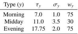
Type (y) τy σy wy

Morning 7.0 1.0 75

Midday 11.0 3.5 30

Evening 17.75 2.0 75

Table 1: Fare profile function parameters

ing”), and compared between two days to give an indication of variability.

Both days showed morning and evening peaks at the same time (around 7am and 6pm respectively, which appear to be very close to the peaks in Figures 2 and 4 of Koppelman et al. (2008)). Both also showed soft midday peaks. However there was significant variation between the two days in terms of rela-tive fare values: Tuesday’s morning peak was much higher than its evening peak, whereas the two peaks for Wednesday (see Figure 2), were of similar height (see Evans (2009) for further details).

The data for these two days was fitted with a combination of 3 normal distribution functions, one for each of the morning, midday and evening peaks, i.e. we constructed

f (t)=ha(t)+hm(t)+he(t)

where each function took the form

hy(t)=wyexp(−

(t−τy)2

2σ2

y

)+80

for each y∈ {a,m,e}, whereτyandσyare the two normal

dis-tribution function parameters (representing mean and standard deviation respectively), and wyis a weighting factor. ($80 was

the “baseline” fare for this route.) The parameters found to best fit the two days of data are shown in Table 1, and resulting func-tion f is shown in Figure 2.

4. Demand allocation

The final step of our approach is to partition market demand Do_,gfor each OD pair, (o,g), (calculated in our first paper

Akar-tunalı et al. (2009a)), amongst the passenger groups for that OD pair. We call this step demand allocation.

For each time-insensitive group g the number of passengers associated with this group,ηg, is simply

ηg =φtm insDog,dg

whereφtm insis the fixed proportion of time-insensitive

passen-gers, unless no other passenger groups were generated for this OD pair. The latter case could occur if the surrogate demand for the OD-pair is very low, in which caseμo,dexceedsT/2. If

this occurs, the time-insensitive group is the only group for its OD pair, and so we setηgto the entire market demand:

ηg=Dog,dg.

As for the peak fare calculation, for time-sensitive groups we use a standardized demand profile: a function d(t) for each t∈[0,T] that indicates the proportion of demand seen at time t. We discuss below how we arrive at this function. The function is normalized so that the area under the curve is 1, and then the number of passengersηgassociated with passenger group g∈G

is calculated as follows:

ηg =(1−φtm ins)Dog,dg( ¯te

g

t=¯ts g

d(t)dt).

We note that for both the fare and demand profiles, our main motivation for using standardized profiles is the lack of ade-quate data to support alternatives. Whilst passenger load data is generally more readily available than fare data, both types of data can only represent preferences for the offered itineraries, which for many OD pairs can be very infrequent. By contrast data derived from passenger surveys would be ideal for our pur-poses. However the literature in this area is quite sparse, (e.g. Walker (2006), Garrow et al. (2007)), and the data collected to date is not rich enough to allow us to differentiate demand pro-files by OD pair characteristic (with the possible exception of travel direction, which we discuss further below). Since this seems to be emerging as a growing field of research, we hope in the future studies will be carried out that will permit greater differentiation of OD pairs. In the meantime, we adopt stan-dardized profiles as a pragmatic approach that we believe yields realistic data useful for optimization benchmarks.

Finding the standardized demand profile. To determine the func-tion d(t), our industry partner analysed the same shuttle route data as was used for deriving the fare profile (see Evans (2009) for more detail). In this case, the number of flights per hour was recorded across each of the two days investigated. The data for one of those days is plotted in Figure 3. Again, the data showed strong morning and evening peaks, with a soft midday peak. Figures 4 and 5 of Garrow et al. (2007) show similar results, with the morning and evening peaks occurring for one type of travellers, and the central peak for another. We thus again seek

Figure 3: Actual and fitted demand profiles

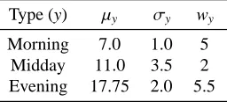
Type (y) μy σy wy

Morning 7.0 1.0 5

Midday 11.0 3.5 2

Evening 17.75 2.0 5.5

Table 2: Demand profile function parameters

to fit a combination of 3 normal distributions to this data, i.e. we construct

ˆd(t)=βa_(t)+βm_(t)+βe_(t)

where each function took the form

βy_(t)=w

yexp(−

(t−τy)2

2σ2

y

)

for each y∈ {a,m,e}, whereτyandσyare the two normal

dis-tribution function parameters (representing mean and standard deviation respectively), and wyis a weighting factor. (d(t) will

be set to ˆd(t) multiplied by a normalizing factor.) The parame-ters found to best fit the two days of data are shown in Table 2, and the resulting function ˆd(t) is shown in Figure 3.

We note that Walker (2006) also suggests approximating the demand distribution by time of day with a combination of nor-mal distributions.

Differentiating by direction of travel. As we have already men-tioned, passengers’ preferred travel time can be affected by the length of the trip, and its direction, in particular if a change in time zone is involved. Research presented by Walker (2006), Garrow et al. (2007) and Evans (2009) suggests that travel time preferences are similar for all directions of travel except for west-to-east, and the difference is more noticeable for travel which includes at least one time zone change, and takes more than 3 hours.

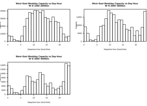
used only included scheduled services, and did not include ac-tual passenger data, so only the available capacity of each leg was used in the analysis. Plots of total flight capacity by local hour of departure are given for all non-west-to-east flights (with net west-east travel less than 750km), broken down by length of trip, in Figure 4. Similar plots for west-to-east travel are shown in Figure 5 (the case of trips less than 1000km is omitted, be-cause it is very similar to the non-west-to-east case).

0 5 10 15 20

0 50000 100000 150000

Non−West−East Weekday Capacity vs Dep Hour Total Distance 0−1000km

Departure hour (local time)

Capacity

0 5 10 15 20

0 20000 40000 60000 80000

Non−West−East Weekday Capacity vs Dep Hour Total Distance 1000−2000km

Departure hour (local time)

Capacity

0 5 10 15 20

0 5000 10000 15000 20000 25000

Non−West−East Weekday Capacity vs Dep Hour Total Distance 2000−3000km

Departure hour (local time)

Capacity

0 5 10 15 20

0 5000 10000 15000

Non−West−East Weekday Capacity vs Dep Hour Total Distance 3000−4000km

Departure hour (local time)

Capacity

Figure 4: Non W-E Capacity versus local hour of departure

0 5 10 15 20

0 10000 20000 30000 40000

West−East Weekday Capacity vs Dep Hour W−E 1000−2000km

Departure hour (local time)

Capacity

0 5 10 15 20

0 5000 10000 15000

West−East Weekday Capacity vs Dep Hour W−E 2000−3000km

Departure hour (local time)

Capacity

0 5 10 15 20

0 2000 4000 6000 8000 10000 12000 14000

West−East Weekday Capacity vs Dep Hour W−E 3000−4000km

Departure hour (local time)

Capacity

Figure 5: W-E Capacity versus local hour of departure

The differences are particularly apparent for trips of greater than 2000km. In these cases, it appears that a significant por-tion of the late afternoon/evening demand is shifted to arrive after 5am instead of before midnight. This may be a natural consequence of airport curfews, or may reflect actual passenger preferences.

Thus we adjust our demand profile function on OD pairs corresponding to long west-to-east trips, by shifting the portion of demand that would arrive between midnight and 5am to the next day. Mathematically, we construct an OD-specific demand

profile

do_,d(t)=

⎧⎪⎪ ⎪⎨ ⎪⎪⎪⎩

d(t)+d(Ts

0+t−T

5am_{), T}5am_≤t≤T5am_+Te

0−T

s

0

0, Ts

0≤t≤T

e

0

d(t), otherwise,

where [Ts

0,T

e

0] is the interval of time during which trips depart-ing o can be expected to arrive at d in the midnight to 5am in-terval, and T5amis obviously 5am in commensurate time units. This is clearly something of an ad hoc adjustment, and in future work, we plan to derive fare and demand profiles, and adjust the timing for types of groups, differentiated by direction and length of travel.

5. Benchmark problems

In this section we present summary statistics of the 33 bench-mark instances created using the methodology described in this paper, taking as input the flight network and OD-pair demand data generated in our first paper Akartunalı et al. (2009a). The complete set of instances and supporting material is available at the URL_{www.infotech.monash.edu.au/~wallace/airline_}

benchmarksalong with the reference Evans (2009).

The 33 instances consist of 30 with a single hub, and 3 with two hubs. The instances are grouped into threes. Each group of three networks were generated using the same parameters except the number of spokes which was varied to provide net-works of different sizes. The instances show a variety of charac-teristics, from small to large in terms of the total passenger mar-ket, flying range, and size of the flight network. They also have differing degrees of asymmetry in the geometry of the flight network, as well as in the OD-pair demand, which also range over the proportion of passengers with an available direct ser-vice, versus those with at best a one-stop service. More details can be found in Akartunalı et al. (2009a).

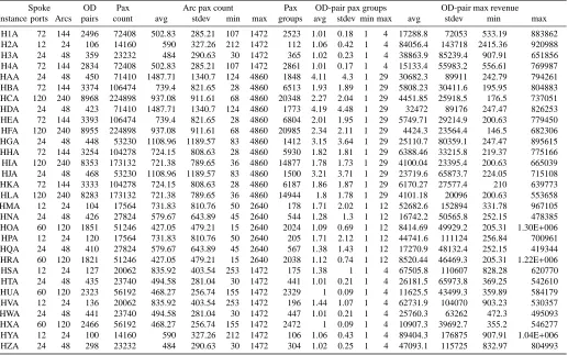
Here in Tables 3 and 4 we show for each instance the flight network size, total number of OD-pair demands, total number of passengers and summary statistics of the passenger load on arcs that was used to infer the OD-pair demand. We also give, in the column “Pax groups”, the total number of passenger groups generated by the methodology we have described here, which ranges from just over 100 up to nearly 21,000 in the largest case. In the four columns headed “OD-pair pax groups” we give summary statistics of the number of passenger groups gen-erated for each OD-pair. These range from 1, meaning that the expected frequency of service on that OD-pair was so low that only the time-insensitive group was generated, to a high of 29. In the final four columns, headed “OD-pair max revenue” we give summary statistics for the total revenue available in each OD-pair market. This is calculated by multiplying the number of passengers in each group by its peak fare, and is the revenue that would be collected if every passenger could be carried at their preferred time of travel.

Spoke OD Pax Arc pax count Pax OD-pair pax groups OD-pair max revenue

Instance ports Arcs pairs count avg stdev min max groups avg stdev min max avg stdev min max

H1A 72 144 2496 72408 502.83 285.21 107 1472 2523 1.01 0.18 1 4 17288.8 72053 533.19 883862

H2A 12 24 106 14160 590 327.26 212 1472 112 1.06 0.42 1 4 84056.4 143718 2415.36 920988

H3A 24 48 359 23232 484 290.63 30 1472 365 1.02 0.23 1 4 38863.9 85239.4 907.91 651856

H4A 72 144 2834 72408 502.83 285.21 107 1472 2861 1.01 0.17 1 4 15133.4 55983.2 556.61 769987

HAA 24 48 450 71410 1487.71 1340.7 124 4860 1848 4.11 4.3 1 29 30682.3 89911 242.79 794261

HBA 72 144 3374 106474 739.4 821.65 28 4860 6513 1.93 1.89 1 29 5808.23 30411.6 195.95 804883

HCA 120 240 8968 224898 937.08 911.61 68 4860 20348 2.27 2.04 1 29 4451.85 25918.5 176.5 737051

HDA 24 48 423 71410 1487.71 1340.7 124 4860 1773 4.19 4.48 1 29 32472 89176 247.47 826253

HEA 72 144 3393 106474 739.4 821.65 28 4860 6804 2.01 1.95 1 29 5749.71 29214.9 200.63 779450

HFA 120 240 8955 224898 937.08 911.61 68 4860 20985 2.34 2.11 1 29 4424.3 23564.4 146.5 682306

HGA 24 48 448 53230 1108.96 1189.57 83 4860 1412 3.15 3.64 1 29 25110.7 80359.1 247.47 895615

HHA 72 144 3254 104278 724.15 808.63 28 4860 5930 1.82 1.81 1 29 6388.46 33215.8 219.37 775166

HIA 120 240 8353 173132 721.38 789.65 36 4860 14877 1.78 1.73 1 29 4100.04 23395.4 200.63 665039

HJA 24 48 468 53230 1108.96 1189.57 83 4860 1500 3.21 3.71 1 29 23719.6 65873.7 224.05 715108

HKA 72 144 3333 104278 724.15 808.63 28 4860 6187 1.86 1.87 1 29 6170.27 27577.4 210 639773

HLA 120 240 8283 173132 721.38 789.65 36 4860 14944 1.8 1.78 1 29 4101.18 20096 200.63 553658

HMA 12 24 104 17564 731.83 810.76 50 2640 178 1.71 2.02 1 12 52682.6 152894 331.78 967105

HNA 24 48 426 27824 579.67 643.89 45 2640 544 1.28 1.3 1 12 16742.2 50565.8 252.15 478385

HOA 60 120 1851 51246 427.05 479.21 15 2640 2024 1.09 0.69 1 12 8414.69 49929.2 205.31 1.30E+006

HPA 12 24 120 17564 731.83 810.76 50 2640 205 1.71 2.12 1 12 44741.6 111124 256.84 700961

HQA 24 48 410 27824 579.67 643.89 45 2640 567 1.38 1.43 1 12 17270.9 48132.4 252.15 419344

HRA 60 120 1821 51246 427.05 479.21 15 2640 2038 1.12 0.74 1 12 8520.44 46469.3 205.31 1.22E+006

HSA 12 24 127 20062 835.92 403.54 253 1472 175 1.38 1 1 4 67505.8 110607 828.28 620770

HTA 24 48 435 23740 494.58 281.04 30 1472 441 1.01 0.21 1 4 26181.5 65973.8 369.25 542610

HUA 60 120 2323 56192 468.27 256.74 155 1472 2329 1 0.09 1 4 11625.5 43499.3 359.89 584179

HVA 12 24 136 20062 835.92 403.54 253 1472 196 1.44 1.07 1 4 62731.9 104070 903.23 530357

HWA 24 48 441 23740 494.58 281.04 30 1472 447 1.01 0.21 1 4 25760.3 63262 472.3 495093

HXA 60 120 2466 56192 468.27 256.74 155 1472 2472 1 0.09 1 4 10907.3 39692.7 355.2 546277

HYA 12 24 100 14160 590 327.26 212 1472 106 1.06 0.43 1 4 89404.3 176875 907.91 1.04E+006

HZA 24 48 298 23232 484 290.63 30 1472 304 1.02 0.25 1 4 47093.1 115725 832.97 804993

Table 3: Summary statistics for single hub benchmark instances

Spoke OD Pax Arc pax count Pax OD-pair pax groups OD-pair max revenue

Instance ports Arcs pairs count avg stdev min max groups avg stdev min max avg stdev min max

HAB 22 74 443 94290 1274.19 1030.61 167 4860 2395 5.41 4.12 1 29 29889.6 78788.8 78.85 631689

HCB 70 226 3340 184406 815.96 888.14 25 4860 9654 2.89 2.5 1 29 8065.79 41779.7 50.5 693051

HEB 118 378 8315 287234 759.88 825.93 35 4860 20236 2.43 2.27 1 29 5308.71 38921.2 50.5 1.32E+006

6. Conclusions and future work

In this paper, we have argued that market segmentation and the use of passenger groups represent a natural “next step” in passenger choice models for use in airline planning optimiza-tion. We have described one approach to defining such groups, which attempts to balance sometimes divergent empirical in-sights against what can practically be instantiated using cur-rently available data. We have presented a methodology by which realistic passenger group data can be generated from a given flight network and OD-pair demands, and produced 33 benchmark instances exhibiting a range of characteristics use-ful for testing optimization algorithms.

The data we have presented here can be used immediately for testing alternative passenger choice models, provided an air-line schedule is also available. We intend in future work to gen-erate schedules to accompany this data, indeed Akartunalı et al. (2009b) explores first steps in this direction. Clearly the gen-eration of realistic schedules depends on the available airline resources. While much data on aircraft types and configura-tions, airline fleets, and operating costs is publicly available, in future work, we plan to extend our benchmark data to include aircraft, and so provide complete sets of input data for the flight schedule design process. We hope that in doing so we can stim-ulate further research in this hitherto less-studied area of airline planning.

Acknowledgements

The authors are very grateful to Ian Evans and Alan Dormer (CTI Pty Ltd) for their ongoing support and guidance on a vari-ety of practical airline-related issues and for numerous techni-cal suggestions and insightful feedback that improved the con-tent and exposition of this work. This research is supported by the Australian Research Council, under Linkage Projects LP00668076 and LP0883855, and by CTI Pty Ltd.

Akartunalı, K., Boland, N., Evans, I., Wallace, M., Waterer, H., 2009a. Airline planning benchmark problems. Part I: Characterizing networks and demand with limited data. Tech. rep., University of Newcastle.

Akartunalı, K., Boland, N., Evans, I., Wallace, M., Waterer, H., Smith, O., 2009b. Airline schedule design: Network design optimization and heuris-tics. Working paper, The University of Melbourne.

Bazargan, M., 2004. Airline Operations and Scheduling. Ashgate Publishing Ltd.

Civil Aviation Authority, 2008. CAA passenger survey report. Tech. rep., Eco-nomic Regulation Group.

Coldren, G., Koppelman, F., Kasturirangan, K., Mukherjee, A., 2003. Modeling aggregate air-travel itinerary shares: logit model development at a major US airline. Journal of Air Transport Management 9, 361–369.

Commission of the European Communities, 2007. Ryanair/Aer Lingus merger procedure report. Office Journal of the European Union Case No COMP/M.4439.

Evans, I., 2009. Typical airline demand and fare profiles. Tech. rep., Constraint Technologies International.

Garrow, L., Jones, S., Parker, R., 2007. How much airline customers are will-ing to pay: an analysis of price sensitivity in online distribution channels. Journal of Revenue and Pricing Management 5, 271–290.

Klabjan, D., 2005. Large-scale models in the airline industry. In: Desaulniers, G., Desrosiers, J., Solomon, M. M. (Eds.), Column Generation. Springer, pp. 163–196.

Kniker, T. S., 1998. Itinerary-based airline fleet assignment. Ph.D. thesis, Mas-sachusetts Institute of Technology.

Koppelman, F., Coldren, G., Parker, R., 2008. Schedule delay impacts on air-travel itinerary demand. Transportation Research Part B 42, 263–273. Lohatepanont, M., Barnhart, C., 2004. Airline schedule planning: Integrated

models and algorithms for schedule design and fleet assignment. Transporta-tion Science 38 (1), 19–32.

UK Department of Transport, 2006. National travel survey: 2006. Tech. rep.,

http://www.dft.gov.uk/adobepdf/162469/221412/221531/223955/322743/NTS2006V3.pdf. Walker, J., 2006. Time of day in airline passenger demand, presentation at the

INFORMS Annual Meeting, Pittsburgh PA.

Yan, S., Tang, C.-H., Lee, M.-C., 2007. Aflight scheduling model fortaiwan airlines under market competitions. Omega 35 (1), 61–74.