MA Alrmah
∗, S Weiss
∗, S Redif
∗∗, S Lambotharan
†, JG McWhirter
‡∗Department of Electronic and Electrical Engineering, University of Strathclyde, Glasgow, Scotland ∗∗Electronic & Electrical Engineering Department, European University of Lefke, Lefke, Cyprus †School of Electronic, Electrical and Systems Engineering, Loughborough University, Loughborough, UK
‡School of Engineering, University of Cardiff, Cardiff, Wales
{mohamed.alrmah,stephan.weiss}@strath.ac.uk, [email protected], [email protected], [email protected]
Abstract. This paper reviews and compares three different linear algebraic signal subspace techniques for angle of
arrival estimation. These include a polynomial matrix approach to multiple signal classification (MUSIC), a parameterised spatial covariance matrix approach, and an auto-focussing based version of coherent signal subspace estimation applied to MUSIC. These approaches are expressed in the framework of polynomial space-time covariance matrices and their polynomial eigenvalue decomposition, thus highlighting their commonalities and differences. Simulation results comparing the accuracy of these broadband angle of arrival estimation methods are presented.
1. Introduction
Powerful narrowband angle of arrival (AoA) estimation meth-ods, such as the multiple signal classification (MUSIC) algo-rithm [1], are not directly applicable to the broadband case, where time delays rather than phase shift need to be considered in distinguishing between spatially separated sources. Narrow-band approximations to the broadNarrow-band case, such as perform-ing the MUSIC algorithm independently in frequency bins, does not work well if sources are coherent [2] or signal fre-quencies do not coincide with frequency bins, leading to poor worst-case performance scenarios [3].
Dedicated broadband AoA estimation algorithms include the coherent signal subspace (CSS) method [2,4], which combines covariance matrices at different frequency bins coherently by means of focussing matrices. The focussing matrices, in their simplest form, pre-steer the data such that the signal of interest appears towards broadside, where narrowband methods suf-fice for estimation. Determining the focussing matrices usu-ally requires a degree of knowledge of the scenario prior to estimation. A recent approach to auto-focussing [5] claims to overcome this problem, and is based on a bin-wise eigenvalue decomposition of covariance matrices.
Further broadband approaches include a recent parameterised spatial covariance (PSC) approach [6,7] which also pre-steers the data to then form a narrowband covariance matrix, and a subspace approach [8] derived from a polynomial eigenvalue decomposition of the space-time covariance matrix [9], which has been employed to generalise MUSIC to the broadband case.
This paper analyses the auto-focussing, parameterised spatial covariance matrix, and polynomial MUSIC approaches in the framework of polynomial space-time covariance matrices and broadband steering vectors. To achieve this, the broadband
array model, and resulting steering vectors and covariance matrix are introduced in Sec. 2.. Broadband approaches to AoA estimation are outlined in Sec. 3. and, together with Sec. 4., formulated within a polynomial matrix framework. A simulation comparison between the different methods is then performed in Sec. 5., with conclusions being drawn in Sec. 6..
Notation. Matrix and vector quantities are represented by upper- and lowercase bold variables, e.g.Aanda. The Her-mitian transpose of A is denoted as AH. Polynomial
vec-tors and matrices are written as a(z) and A(z), with the parahermitian ˜A(z) =AH(z−1). A transform pair a[n] and A(z) =∑∞n=−∞a[n]z−nis abbreviated asa[n]◦—•A(z).
2. Broadband Steering Vectors and Space-Time Covari-ance Matrix
Below, we define a steering vector to characterise a source in a broadband scenario in Sec. 2.1, which is used to define a polynomial space-time covariance matrix in in Sec. 2.2 and its polynomial eigenvalue decomposition in Sec. 2.3.
2.1 Broadband Steering Vector
Given an array ofM-element containing omnidirectional sen-sors located at positionsrm,m=1. . .M, a signal vectorx[n],
x[n] =
δ[n−∆τ1] δ[n−∆τ2]
.. .
δ[n−∆τM]
∗ s[n] =a[n]∗s[n] , (1)
is collected if the array is illuminated by a source. We assume that the source signal measured at the origin iss[n], with ∗
wherecis the propagation speed in the medium, fsis the
sam-pling rate,kis the normal vector of the source’s wave front, andk/cis known as the slowness vector of the source. The delays δ[n−∆τ] are generally fractional delays [10], implementable e.g. via sinc functions sampled off their zero-crossing,δ[n−∆τ] =sinc[n−∆τ], whilea[n]in (1) is referred to as a broadband steering vector. The later, through the nor-mal vectork’s dependence on azimuthϕand elevationϑ,
kϕ,ϑ =
cosφsinθ
sinφsinθ
cosθ
, (2)
defines the spatial characteristics of a far-field source, and will also be denoted asaϑ,ϕ[n].
2.2 Polynomial Space-Time Covariance Matrix
In a scenario withLindependent far field broadband sources
sl[n],l =1. . .L, each characterised by a broadband steering
vectoral[n], the signal model becomes
x[n] =
L
∑
l=1al[n] ∗ sl[n] + v[n] , (3)
with v[n] representing spatially and temporally uncorrelated noise with covarianceE
v[n]vH[n] =σ2
vI. To capture
infor-mation contained in the data vectorx[n]requires a space-time covariance matrixR[τ] =E
x[n]xH[n−τ] with lag
parame-terτ. The cross-spectral density matrixR(z) = •—◦R[ν],
R(z) =
L
∑
l=1a(z)aH(z−1)Rl(z) +σ2
vI (4)
withRl(z)the power spectral density of thelth source, forms a
polynomial matrix.
2.3 Space-Time Covariance Matrix and Polynomial Eigen-value Decomposition
The power spectral matrix in (4) can be decomposed to yield a polynomial EVD [9]
R(z) =Q(z)Λ(z)Q˜(z) =
M−1
∑
m=0λm(z)qm(z)q˜m(z) (5)
with paraunitaryQ(z), i.e.Q(z)Q˜(z) =I. The matrixΛ(z)is diagonal and contains polynomial eigenvaluesλm(z), which
are spectrally majorised, such that
λm(ejΩ)≥λm+1(ejΩ) ∀Ω ,m=0. . .(M−2) . (6)
Thresholding the eigenvalues reveals the number of indepen-dent broadband sources contributing toR(z), and permits a dis-tinction between signal-plus-noise and noise only subspaces
R(z) = [Qs(z)Qn(z)]
Λs(z) 0 0 Λn(z)
QHs(z)
QH
n(z)
(7)
similar to a narrowband EVD [11]. Specifically, the nullspace ˜
Qn(z)
˜
Qn(z) =
˜
qL(z)
.. . ˜
qM−1(z)
(8)
is spanned by vectors ˜qL(z)which have the same appearance
as broadband steering vectors.
3. Broadband Angle of Arrival Estimation
In analysing broadband AoA estimation approaches, we first review the parameterised spatial covariance matrix method [6,7] in Sec. 3.1, followed by an auto-focussing approach [5] to coherent signal subspace-based estimation in Sec. 3.2 and polynomial MUSIC [8] in Sec. 3.3.
3.1 Parameterised Spatial Correlation (PSC) Matrix Method
The idea of the broadband AoA estimation method in [6,7] is based on testing the zero-lag coherence of a spatial correlation matrix calculated from appropriately pre-steered array data. Knowing the array configuration, a broadband steering vector can be defined for a specific AoA represented by azimuthϕ
and elevation ϑ, and pre-steering can be accomplished by a matched broadband steering vector. The covariance matrix of the pre-steered data is given by
Rϕ,ϑ = E
n
yϕ,ϑ[n]yHϕ,ϑ[n]
o
(9)
yϕ,ϑ[n] =
x[n−∆τ0(ϕ,ϑ)] .. .
x[n−∆τM−1(ϕ,ϑ)]
=Γϕ,ϑ[n]∗x[n] (10)
with the delay∆τm(ϕ,ϑ)calculated akin to Sec. 2.1, and the
diagonal pre-steering system
Γϕ,ϑ[n] =diag{δ[n−∆τ0(ϑ)]. . .δ[n−∆τM−1(ϑ)]}. (11)
The proposed method then evaluates the maximum eigenvalue ofRϕ,ϑin (9) for a range of angles{ϕ,ϑ}, with the best match
indicated by {ϕopt,ϑopt} = arg maxϕ,ϑ{maxiλi(Rϕ,ϑ)},
whereλi(Rϕ,ϑ)denotes theith eigenvalue ofRϕ,ϑ.
In terms of the space time covariance matrix and broadband steering vectors defined in Sec. 2., the problem can formulated as
{ϕopt,ϑopt}=argmax
ϕ,ϑ{maxi λi(
ˆ
Rϕ,ϑ[0])} (12)
with ˆRϕ,ϑ[0]being the evaluation for lag zero of the space-time
covariance matrix ˆRϕ,ϑ[τ]◦—•Rˆϕ,ϑ(z)
ˆ
Rϕ,ϑ(z) =diagaϕ,ϑ(z) R(z)diaga˜ϕ,ϑ(z) (13)
3.2 Coherent Signal Subspace Method
In the coherent signal subspace approach [2,4], covariance matrices are calculated in a number of frequency bins, which are then coherently combined such that their signal subspaces align into one single scalar-valued correlation matrix to which narrowband high resolution AoA techniques such as MUSIC can be applied. The coherence across different frequency bins is created by a frequency-dependent and unitary focussing matrixT(ejΩ), such that
Rcoh=
N−1
∑
i=nαnT(ejΩn)R(ejΩn)TH(ejΩ) , (14)
whereαn a weighting for maximum ratio combination of its
coherently rotated contributions. The calculation of focussing matrices in the context of coherent signal subspace methods can be based on approximate knowledge of the AoA of the source of interest, or be obtained numerically by a best fit of a rotatedT(ejΩn)to a referenceT(ejΩo), whereby the rotation forms the focussing matrix.
A recent auto-focussing method in [5] calculates, based on a reference frequencyΩ0, an EVD of the appropriate
frequency-bin covariance matrixR(ejΩ0),
Λo=QH0R(ejΩ0)Q0 . (15)
Extracting the modal matrix for frequency bink,k=0. . .(K−
1), the auto-focussing matrix is constructed according to
T(ejΩk) =Q
0QH(ejΩk) . (16)
Therefore, the coherent covariance matrix in (14) can be diag-onalised byQ0to provide
Λcoh=QH0RcohQ0=diag{λ1 λ2 . . . λM} , (17)
with λm,m=1. . .M the eigenvalues ofRcoh in (14). If the
eigenvaluesRcoh revealR linearly independent sources, then
the last M−R columns of Q0=
h
Q0,sQ⊥0,s
i
contained in
Q⊥0,s∈CM×(M−R)span the noise-only subspace of the coherent covariance matrix.
The standard narrowband MUSIC algorithm [1] can be applied toRcoh by probing its noise-only subspaceQ⊥0,s with a set of
narrowband steering vectors at the reference frequency Ω0.
Based on the transform domain broadband steering vector
aϕ,ϑ(z)at the reference frequencyΩ0, the MUSIC spectrum
for auto-focussing (AF)
SAF(ϕ,ϑ) =kQ⊥0,saϕ,ϑ(ejΩ0)k−22
= 1
aH
ϕ,ϑ(ejΩ0)Q⊥
,H
0,s Q⊥0,saϕ,ϑ(ejΩ0)
(18)
is obtained.
3.3 Polynomial MUSIC Algorithm
Generalising the concept of the narrowband MUSIC algorithm by using the polynomial EVD in (7), the idea is to probe the broadband noise-only subspace with broadband steering vec-tors, generalised quantity
Γϕ,ϑ(z) =a˜ϕ,ϑ(z)Qn(z)Q˜n(z)aϕ,ϑ(z) .
Noting that (3.3) represents a power spectral density rather than a norm measuring the vicinity ofaϕ,ϑ(z)to the nullspace
of ˜Qn(z), two versions of the a polynomial MUSIC
(P-MUSIC) algorithm were proposed in [8], which are outlined below.
Spatial P-MUSIC.The energy contained in the signal vector ˜
Qn(z)aϕ,ϑ(z)is related to the zero lag termγϕ,ϑ[0]of the
auto-correlation-type sequenceγϕ,ϑ[τ]◦—•Γϕ,ϑ(z). This measure
is only dependent on the angle of arrivalϑ, and collects all energy across the spectrum. Instead of searching for the steer-ing vectors providsteer-ing minimum energy, the reciprocal
SPS(ϕ,ϑ) =
1
γϕ,ϑ[0]
. (19)
is maximised by the angle of arrival characterised by the azimuth/elevation pair{ϕ,ϑ}of signal sources.
Spatio-Spectral P-MUSIC.With (3.3) describing a power spec-tral density, specspec-tral clues can be exploited in addition to the spatial information extracted by (19). Therefore in addition to spatial localisation of sources,
SPSS(ϕ,ϑ,Ω) =
∞
∑
τ=−∞
γϕ,ϑ[τ]e−jΩτ
!−1
(20)
can determine over which frequency range sources in the direc-tion defined by the steering vector aϕ,ϑ(z) are active.
PSS-MUSIC was introduced in [8], but will be omitted from the comparison below, since the benchmark method only retrieves AoA information.
4. Analytical Comparison
The auto-focussing approach to coherent signal subspace esti-mation is linked to the polynomial EVD of the space-time covariance matrix in Sec. 4.1, while Secs. 4.2 and 4.3 relate the auto-focussing approximation of coherent signal subspace MUSIC to the polynomial PSS- and PS-MUSIC methods in [8].
4.1 Auto-Focussing Matrices via Polynomial Eigenvalue Decomposition
With the modal matrix Q0 in (16) obtained at the reference
frequencyΩ0via EVD ofR(ejΩ0), the focussing matrix can be
Replacing the summation over frequency bins in (14) by the integration over the Fourier transform (i.e.K→∞) leads to
Rcoh≈
1 2π
I
T(z)R(z)T˜(z) z=ejΩdΩ (21)
=Q0
1 2π
I
˜
Q(z)R(z)Q(z) z=ejΩdΩQH0. (22)
Since the paraunitary matrix Q(z) diagonalises R(z), the argument under the integral is the polynomial EVD in (5), resulting in a diagonal matrix of power spectral densi-ties, 2π1 H
Γ(ejΩ)dΩ=Γ[0], where Γ[0] is the evaluation of
Γ[τ]◦—•Γ(z)for zero lag. Therefore
Rcoh≈Q0Γ[0]QH0 =Q0
σ2 1
. ..
σ2
M
Q
H
0 (23)
represents the coherent covariance matrix of the auto-focussing approach in terms of the polynomial EVD of the cross spectral density matrix.
Given that the DFT in (14) is a sufficiently accurate representa-tion of the Fourier transform formularepresenta-tion in (21), then (17) and (23) are equivalent withΛ=Γ[0]. Further, the PEVD of the CSD matrix provides a paraunitaryQ(z)that leads to an auto-focussing matrixQ0Q˜(z)which is continuous in frequency.
4.2 Relation between Auto-Focussing MUSIC and PSS-MUSIC
Provided that the estimation of the number of linearly indepen-dent sources,R, is the same for the auto-focussing approach of CSS and from (23) of the polynomial approach, then withQ0
being the evaluation of the paraunitaryQ(z)at the reference frequencyΩ0, i.e.Q0=Q(z)|z=ejΩ0, it follows that
SCSS(ϕ,ϑ) =SPSS(ϕ,ϑ,ejΩ)|Ω=Ω0 . (24)
Therefore, the auto-focussing approach to coherent signal sub-space MUSIC estimation is equivalent to evaluating the poly-nomial spatio-spectral MUSIC spectrum at the reference fre-quencyΩ0.
To obtain the same spatio-spectral characterisation of the array data as provided by PSS-MUSIC with the CSS approach, a sequence of different modal matricesQ0at different reference
frequencies Ω0 could be calculated, for all of which (18) is
evaluated.
4.3 Relation between Auto-Focussing MUSIC and PS-MUSIC
Noting that in (19),
γϕ,ϑ[0] = 1
2π 2π
I
0
Γϕ,ϑ(ejΩ)dΩ , (25)
if the integral can be approximated by a sum over discrete fre-quency bins, i.e.
γ≈K1
K−1
∑
k=0aHϕ,ϑ(ejΩk)Q⊥,H
s (eΩk)Q⊥s(ejΩk)aϕ,ϑ(ejΩk), (26)
then (26) is the summation over the denominator terms of (18) for all possible reference frequenciesΩkwithΩk=2πKk,
k=0. . .(K−1). The PS-MUSIC denominator in the above approximation also appears similar to the incoherent MUSIC approach stated in [12]; however, here the paraunitary matrix
Q(z) that feeds into (26) has been demonstrated in (23) to coherent combine the spatio-temporal covariance matrix in the auto-focussing sense.
5. Simulations and Numerical Results
Below, we illustrate the analysis of the above broadband AoA estimation algorithms in two examples.
5.1 Example 1 — Single Source Case
To highlight the connection between the auto-focussing approach and PSS-MUSIC, we first consider a simple toy problem with a single source in a noise-free environment, where the space-time covariance matrix and its ideal decom-position are known. Here, a single broadband source emits an uncorrelated Gaussian signal, which is captured by anM=4 element linear array with equispaced sensors that sample criti-cally in both time and space. The broadband steering vector of this source is
a1(z) =
1
√ M [1 z
−1 . . . z−M+1]T (27)
such that the space-time covariance matrix is given by
R1(z) =
1 z1 . . . zM−1
z−1 1 ...
..
. . .. ...
z−M+1 . . . . 1
. (28)
BecauseR1(z)is rank one, a manifold of diagonalising
poly-nomial decompositions exists, with one possibility being
Q(z) =diag
1z−1. . .z−M+1 TDFT, (29)
whereTDFTis anM-point DFT matrix normalised by √
Msuch thatTDFT is unitary. Based on PSS-MUSIC in (??) using a
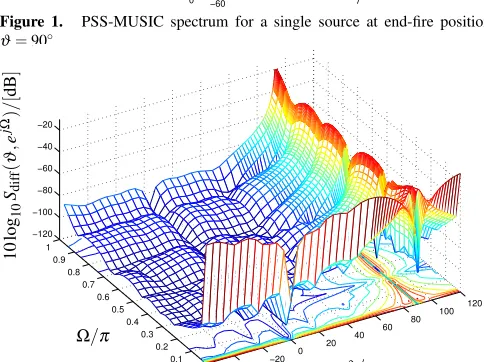
sampled sinc function, truncated to order 200, to approximate broadband steering vectors, the spectrum in Fig. 1 emerges. Normalised to a maximum value of unity, the AoA of the end-fire source is identified. In line with broadband arrays, at lower frequencies the fixed aperture degrades the spatial resolution, with no ability to discern sources at DC.
−60 −40 −20 0 20 40 60 80 100 120 0 0.1 0.2 0.3 0.4 0.5 0.6 0.7 0.8 0.9 1 −80 −60 −40 −20 0
Ω/π
ϑ/◦
[image:5.595.315.542.96.267.2]1 0 lo g1 0 SP S S ( ϑ , e j Ω) / [ d B ]
Figure 1. PSS-MUSIC spectrum for a single source at end-fire position,
ϑ=90◦.
−60 −40 −20 0 20 40 60 80 100 120 0 0.1 0.2 0.3 0.4 0.5 0.6 0.7 0.8 0.9 1 −120 −100 −80 −60 −40 −20
Ω/π
ϑ/◦
1 0 lo g1 0 Sd if f ( ϑ , e j Ω) / [ d B ]
Figure 2. Difference between the PSS- and auto-focussing (AF) based
MUSIC spectra for a single source atϑ=90◦.
Evaluating the narrowband MUSIC algorithm using narrow-band steering vectors atΩ0for a range ofK=64 discrete
equi-spaced reference frequenciesΩ0, and the nullspaceQ⊥s (ejΩ0)
derived from the EVD ofRcoh,Ω0, a MUSIC spectrum similar to Fig. 1 emerges.
The difference between the PSS- and AF-MUSIC spectra,
Sdiff(ϑ,ejΩ) =|SPSS(ϑ,ejΩ)−SAF(ϑ,Ω)|, is plotted in Fig.2,
with an error below -10dB. The error is largest where the MUSIC spectrum is numerically most sensitive, i.e. towards the source atϑ =90◦, and for DC, Ω=0. The error can be attributed to the inaccuracies of the truncated sinc functions to implement fractional delays for the broadband steering vector, while narrowband steering vectors required for CSS-MUSIC can always be accurately represented. Note that for the trivial broadband steering vector towards broadside,
a0◦(z) =M1[1 1. . .1]T, the error in Fig. 2 forϑ =0◦is
negli-gible.
For this case with a single source and known covariance matrix, the integration of the PSS-MUSIC spectrum across frequency yields the PS-spectrum, which in Fig. 3 is shown for both the correct PEVD and its iterative approximate solu-tion using the second order sequential best rotasolu-tion algorithm (SBR2) [9]. The significant degradation is due to the sensitivity
−600 −40 −20 0 20 40 60 80 100 120
0.2 0.4 0.6 0.8 1 ϑ/◦ n o rm a li se d sp ec tr u m PSC
AF -MUSIC (Ω0=π/2)
AF -MUSIC (integrated) PS-MUSIC (SBR2) PS-MUSIC (ideal)
87 88 89 90 91 92 93
0 0.2 0.4 0.6 0.8 1 ϑ/◦ n o rm a li se d sp ec tr u m PSC
AF -MUSIC (Ω0=π/2)
[image:5.595.43.282.106.267.2]AF -MUSIC (integrated) PS-MUSIC (SBR2) PS-MUSIC (ideal)
Figure 3. Comparison between PSC, AF-MUSIC (i) evaluated at the centre
frequencyΩ0=π2 and (ii) integrated according to (26), and PS-MUSIC (iii) with SBR2-estimated and (iv) ideal PEVD; the bottom graph shows a detail of the overall response in the top figure.
of the MUSIC algorithm to small modifications of the denom-inator when close to zero. It can be seen that the difference to the integrated CS-MUSIC is very small. As a benchmark, the parameterised spatial covariance matrix approach [6,7] is also plotted in Fig. 3. Unlike the MUSIC approaches, PSC does not display an inverse value, and hence will not exhibit the same sharp peaks and at least appear to possess a much lower resolution in comparison.
5.2 Example 2 — Dual Source Case
In addition to a source at end-fire, a second independent source is assumed to illuminate from broadside,ϑ =0◦. Assumed to be temporally uncorrelated with unit variance, its broadband steering vector is
a2(z) =
1
√
M [1 1 . . . 1]
T ,
(30)
leading to a non-polynomial space-time covariance matrix with unity for all entries. With a relative signal strength of 0dB for each source, additional i.i.d. noise contaminates all sensors at a variance of -20dB, giving an SINR of -23dB. Therefore the overall space-time covariance is
R2(z) =R1(z) +
1
M
1 1 . . . 1 ..
. . .. ... 1 1 . . . 1
+σ
2
vI, (31)
with no obvious PEVD as forR1(z)in (29).
[image:5.595.43.285.268.449.2]Ω/π
ϑ/◦
1
0
lo
g1
0
SP
S
S
(
ϑ
,
e
j
Ω)
/
[
d
B
[image:6.595.317.538.96.242.2]]
Figure 4. PSS-MUSIC spectrum for sources at broadside (ϑ=0◦) and end–
fire (ϑ=90◦).
−60 −40 −20 0
20 40 60 80
100 120
0 0.1 0.2 0.3 0.4 0.5 0.6 0.7 0.8 0.9 1 −40 −30 −20 −10 0
Ω0/π
ϑ/◦
1
0
lo
g1
0
SA
F
(
ϑ
,
Ω0
)
/
[
d
B
]
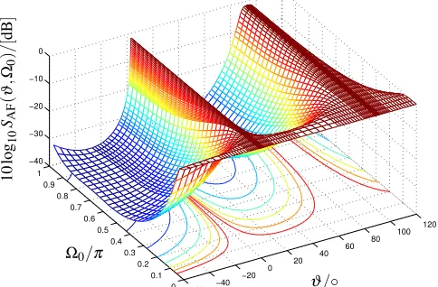
Figure 5. AF-MUSIC spectrum evaluated over a range of reference
frequen-ciesΩ0for the scenario in Fig. 4.
The spatial-only spectra for the dual source case in Fig. 6 illustrate, that PSC is only able to resolve a single source, while AF- and PS-MUSIC approaches correctly detect the sources, with AF offering a higher resolution due to the SBR2-approximation of the ideal PEVD for the PS-MUSIC case.
6. Conclusions
Three broadband angle of arrival estimation algorithms have been reviewed and analysed, including a parameterised spa-tial covariance matrix approach, which by definition can only resolve the strongest source, an auto-focussing approximation of the coherent signal subspace method, where the broadband problem is transformed to yield a narrowband one, and a poly-nomial MUSIC approach. The algorithms have been cast in the framework of broadband steering vectors and broadband space-time covariance matrices, and the links in particular between the auto-focussing approach and polynomial MUSIC have been stated, which generally rely on the transition from a discrete evaluation of frequency bins to a continuous spec-trum. In simulations, AF- and polynomial MUSIC approaches have proven very similar, with differences arising from the iterative approximation of the polynomial EVD. However, a
−80 −60 −40 −20 0 20 40 60 80
−50 −45 −40 −35 −30 −25 −20 −15 −10 −5 0 5
θ / [o]
spectrum /[dB]
[image:6.595.52.291.101.269.2]PCM PS AF
Figure 6. PSC compared to PS- and AF-spectra, normalised to unity, for the
dual source case.
natural advantage of the polynomial MUSIC approach is its potential resolution of both angle of arrival and frequency.
References
[1] R. O. Schmidt, “Multiple emitter location and signal parameter estimation,”IEEE Transactions on Antennas and Propagation, vol. 34, no. 3, pp. 276–280, March 1986.
[2] H. Wang and M. Kaveh, “Coherent signal-subspace processing for the detection and estimation of angles of arrival of multiple wide-band sources,”IEEE Transactions on Acoustics, Speech and Signal Processing, vol. 33, no. 4, pp. 823–831, Aug 1985. [3] S. Weiss and I. K. Proudler, “Comparing Efficient Broadband
Beamforming Architectures and Their Performance Trade-Offs,” in14th International Conference on Digital Signal Pro-cessing, vol. I, Santorini, Greece, July 1–3 2002, pp. 417–422. [4] H. Hung and M. Kaveh, “Focussing matrices for coherent
signal-subspace processing,”IEEE Transactions on Acoustics, Speech and Signal Processing, vol. 36, no. 8, pp. 1272–1281, Aug. 1988.
[5] P. Pal and P. P. Vaidyanathan, “A novel autofocusing approach for estimating directions-of-arrival of wideband signals,” in
Forty-Third Asilomar Conference on Signals, Systems and Computers, Pacific Grove, CA, November 2009, pp. 1663– 1667.
[6] J. Dmochowski, J. Benesty, and S. Affes, “Direction of arrival estimation using the parameterized spatial correlation matrix,”
IEEE Transactions on Audio, Speech, and Language Process-ing, vol. 15, no. 4, pp. 1327–1339, May 2007.
[7] M. Souden, J. Benesty, and S. Affes, “Broadband source local-ization from an eigenanalysis perspective,”IEEE Transactions on Audio, Speech, and Language Processing, vol. 18, no. 6, pp. 1575–1587, August 2010.
[8] M. Alrmah, S. Weiss, and S. Lambotharan, “An extension of the music algorithm to broadband scenarios using polynomial eigenvalue decomposition,” in19th European Signal Process-ing Conference, Barcelona, Spain, August 2011, pp. 629–633. [9] J. G. McWhirter, P. D. Baxter, T. Cooper, S. Redif, and J.
Fos-ter, “An EVD Algorithm for Para-Hermitian Polynomial Matri-ces,”IEEE Transactions on Signal Processing, vol. 55, no. 5, pp. 2158–2169, May 2007.
[10] T. I. Laakso, V. V¨alim¨aki, M. Karjalainen, and U. K. Laine, “Splitting the Unit Delay,”IEEE Signal Processing Magazine, vol. 13, no. 1, pp. 30–60, January 1996.
[11] G. H. Golub and C. F. Van Loan,Matrix Computations, 3rd ed. Baltimore, Maryland: John Hopkins University Press, 1996. [12] Y.-S. Yoon, L. Kaplan, and J. McClellan, “TOPS: new DOA
[image:6.595.50.292.297.456.2]