Scaling Soft Matter Physics to
Thousands of GPUs in Parallel
Alan Gray1, Alistair Hart2, Oliver Henrich1 and Kevin Stratford1
1EPCC, The University of Edinburgh 2Cray Exascale Research Initiative Europe
Keywords: Lattice Boltzmann, Fluid Dynamics, Molecular Dynamics, CUDA, MPI, Parallel Scaling
Abstract
1
Introduction
A wide variety of substances such as mixtures, surficants, particle suspensions and liquid crystals can collectively be classed as soft matter. Everyday examples can be found in foodstuffs, cosmetic and healthcare items, technological products and even components within our bodies. Improving the understanding of such materials is not only interesting from a research perspective but potentially allows the development of new and improved materials. Many soft materials may also be categorised as complex fluids, since they display complex behaviour at the macroscopic level dependent on the physical properties of the structures that self-organise from the fluid components at the microscopic scale.
Ludwig [1] is a versatile software package able to simulate a wide variety of
complex fluids. As a basis, Ludwig uses lattice Boltzmann (LB) fluid dynamics, which is particularly suitable for implementation on large-scale parallel architectures. For complex fluids, this is coupled with other techniques to represent the substance under investigation. A current focus of research interest is liquid crystal (LC) systems [2][3][4]. LCs are perhaps best known from use in liquid crystal displays, but are also found in a variety of other technological items and natural systems. There is still much to be understood about the behaviour of different LC systems under different conditions, and how to harness desirable properties. In particular, the stability of LC systems can potentially be improved through anchoring to colloidal particles. Our aim is to fully understand this phenomenon through the use of Ludwig, but this requires very large and computationally demanding simulations.
Computational resources that augment traditional CPUs with Graphics Processing Units (GPUs) as compute accelerators offer performance advantages over the use of CPUs alone. The world’s largest open-access supercomputer (at the time of writing), Titan at Oak Ridge National Laboratory, exploits more than 18,000 GPUs to achieve this status. However, non-trivial software development is required for applications to efficiently utilise GPUs, especially for use in massively parallel supercomputers. In this paper we describe the work performed to enable Ludwig to utilise large-scale GPU-accelerated architectures to achieve substantial performance improvements over the use of traditional CPUs alone, and make feasible studies such as that mentioned above.
The suitability of GPUs for LB is well established in the literature, from early work using low-level graphics APIs to achieve fluid-like effects in computer animation [5][6][7], through the first NVIDIA CUDA implementation [8] to increasingly sophisticated implementations mixing CUDA with other parallel programming paradigms to allow use of multiple GPUs [9][10][11][12][13][14]. The heterogeneous nature of these systems has also spurred interest in approaches including automatic code generation [15] and auto-tuning [16] to aid application performance. The novelty of the work described in this paper lies in our success in managing the complexities associated with simulating complex
a binary fluid system, noting that the mechanisms and techniques are transferable to other systems including liquid crystals.
In Section 2.1 we briefly introduce the underlying physics, and discuss the implementation within Ludwig. Then, in Section 2.2, we describe how we adapt Ludwig for the GPU architecture, and discuss the optimisations necessary to effectively utilise each GPU. In Section 2.3 we describe how to incorporate colloidal particles into the fluid simulation, in a way that minimises overheads associated with CPU-GPU data transfer. We go on, in Section 2.4, to describe our method for performing the necessary communications required for multi-GPU simulations, where we utilise overlapping to maximise efficiency. Finally, in Section 3 we present performance results on Titan, using up to 8192 GPUs in parallel.
2
Background and Implementation
2.1 Background
For a general complex fluid problem the starting point is the fluid velocity field
𝐮(𝐫), whose evolution obeys the Navier-Stokes equation describing the conservation of mass (or density 𝜌), and momentum:
𝜌 𝜕'𝐮 + 𝐮. ∇ 𝐮 = −∇𝑝 + 𝜂∇/𝐮 + 𝐟(𝐫)
where 𝑝 is the isotropic pressure and 𝜂 is the viscosity. A local force 𝐟(𝐫)
provides a means for coupling to other complex fluid constituents, e.g., it might represent the force exerted on the fluid by a curved interface between different phases or components (see below).
The LB approach makes use of a regular three-dimensional lattice (see Figure 1) with discrete spacing ∆𝑟. It also makes use of a discrete velocity space 𝐜4, where the 𝐜4 are chosen to capture the correct symmetries of the Navier-Stokes equations. A typical choice, used here, is the so-called D3Q19 basis in three dimensions where there is one velocity such that 𝐜∆𝑡 is zero, along with six extending to the nearest neighbour lattice sites, and twelve extending to the next-nearest neighbour sites (∆𝑡 being the discrete time step). The fundamental object in LB is then the distribution function 𝑓4(𝐫; 𝑡), whose moments are related to the local hydrodynamic quantities: the fluid density, momentum, and stress. The time evolution of the distribution function is described by a discrete Boltzmann equation
𝑓4 𝐫 + 𝐜𝒊∆𝑡; 𝑡 − 𝑓4 𝐫; 𝑡 = −ℒ4:𝑓: 𝐫; 𝑡 .
(sometimes referred to as streaming step), in which each element 𝑖 of the distribution is displaced 𝐜𝒊∆𝑡, i.e., one lattice spacing in the appropriate direction per discrete time step.
In order to simulate complex fluids in the Ludwig application, we couple to the above the evolution of an order parameter field which describes the composition of the fluid. The way in which this is done depends on the system of interest: in this paper we concentrate on binary fluid.
For a symmetric binary fluid, in which both components have the same density and viscosity, the order parameter 𝜙(𝐫) is a function of position 𝐫 and describes the relative proportions of the two fluids present locally. To describe the thermodynamics of the system it is possible to write down a free energy which is a functional of the order parameter. The equation of motion for 𝜙 is then
𝜕'𝜙 + ∇. 𝐮𝜙 = −𝛻. (𝑀𝛻𝜇)
where 𝜇 is the chemical potential related to the functional derivative of the free energy, and 𝑀 is a (constant) mobility. To represent the composition variable in our lattice implementation, we introduce a second distribution function 𝑔4(𝐫; 𝑡)
whose first moment is 𝜙, second moment is the order parameter flux, and so on [1]. A solution to the equation of motion can be obtained by evolving this second distribution through an analogous collision and propagation process to that described for 𝑓4 [18]. The order parameter then couples to the evolution of the first distribution function through the local force term 𝐟 𝐫 in the Navier-Stokes equation (which enters the lattice Boltzmann equation within the collision operator). It is sufficient to note here that this force depends locally on the order parameter and its derivatives 𝛻𝜙 and 𝛻/𝜙, which are calculated using standard finite difference techniques. For a full description the interested reader is referred to, e.g.,[19][20].
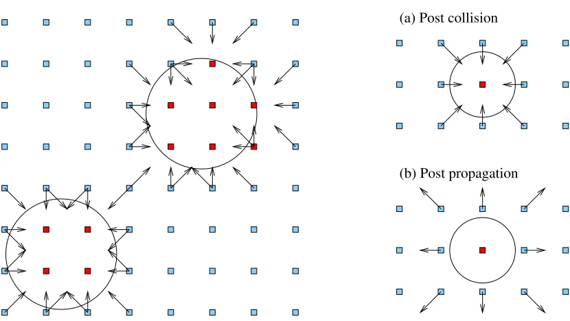
Figure 1: Left: The lattice decomposed between MPI tasks. For clarity we show a 2D decomposition of a 3D lattice, but in practice we decompose in all 3 dimensions. Halo cells are added to each sub-domain (as shown on the upper right for a single slice) which store data retrieved from remote neighbours in the halo exchange. Lower right: the D3Q19 velocity set resident on a lattice site; highlighted are the 5 “outgoing” elements to be transferred in a specific direction.
To allow utilisation of multi-node computing architectures, Ludwig is parallelised using domain decomposition and message passing communications. The regular 3D decomposition is illustrated in Figure 1. Each local sub-domain is surrounded by a halo (or ghost), region. Elements of the distribution must be exchanged at the edges of the domains to facilitate the propagation. To achieve the full 3D halo exchange, the standard approach of shifting the relevant data in each co-ordinate direction in turn is adopted. This requires appropriate synchronisation, i.e., a receive in the first co-ordinate direction must be complete before a send in the second direction involving relevant data can take place, and so on. We note that only “outgoing'” elements of the distribution need to be sent at each edge. For the D3Q19 model, this reduces the volume of data traffic from 19 to 5 of the distribution velocity components per lattice site at each edge. In the CPU version of the code, the necessary transfers are implemented in place using a vector of appropriately strided MPI datatypes for each direction.
2.2 GPU enablement and Optimisation
order to port to the GPU in an incremental fashion, we have tried to maintain the modular structure of the CPU version where possible. For each data structure, such as the distribution, a separate analogue is maintained in both the CPU and GPU memory spaces. However, the GPU copy does not include the complete CPU structure: in particular, non-intrinsic datatypes such as MPI datatypes are not required on the GPU. Functions to marshal data between CPU and GPU are provided for each data structure, abstracting the underlying CUDA implementation. (This reasonably lightweight abstraction layer is a future-proofing measure since it will aid portability to, e.g. an OpenCL implementation.) This makes it easy to switch between the CPU and GPU for different components in the code, which is useful in development and testing. GPU functionality can be added incrementally while retaining a code that runs correctly (albeit slowly due to data transfer overheads). It is necessary to offload all computational activity that involve the main data structures (such as the distribution) to the GPU, including kernels with relatively low computational demand: once all relevant components are moved to the GPU, it becomes possible to remove the data transfers and keep the entire problem resident on the device for the duration of the timestepping algorithm (with the exception of those subsets of data to be marshalled for communication operations or particle interactions, as described later in this paper).
To achieve optimal performance, it is vital to fully exploit the parallelism inherent in the GPU architecture. The GPU architecture features a hierarchy of parallelism. At the lowest level, groups of 32 threads (warps) operate in lock-step on different data elements: this is SIMD style vector-level parallelism. Multiple warps are combined into a thread block (in which communication and synchronisation are possible), and multiple blocks can run concurrently across the streaming multiprocessors in the GPU (with no communication or synchronisation possible across blocks). For most kernels, we find that simply assigning a separate CUDA thread to each lattice site works well, using a CUDA block size of 256. That is, we decompose the lattice into groups of 256 sites, and assign each group to a block of CUDA threads. For kernels such as the collision involving only operations local to each lattice site, we can simply linearize the lattice indexing and perform a 1D CUDA decomposition. For kernels such as the propagation which involve updates based on neighbouring site values, we use a 3D CUDA decomposition. This improves performance since it reduces the number of lattice site memory loads for each thread block (and improves cache utilisation).
An architectural constraint of GPUs means that optimal global memory bandwidth is only achieved when data are structured such that threads within a
half-warp (a group of 16 threads) load data from the same memory segment in a
a choice of distribution data layout at compilation time depending on the target architecture: CPU or GPU. Additionally, for those data that are read-only we exploit the constant cache and texture memory pipe where possible.
[image:7.595.90.505.162.396.2]2.3 Moving Solid Particles
Figure 2: A two-dimensional schematic picture of spherical particles on the lattice. Left: a particle is allowed to move continuously across the lattice, and the position of the surface defines fluid lattice sites (light blue) and solid lattice sites (dark red). The discrete surface is defined by links where propagation would intersect the surface (arrows). Note the discrete shape of the two particles is different. Right: post-collision distributions are reversed at the surface by the process of bounce-back on links, which replaces the propagation.
The introduction of moving solid particles (often called colloidal particles) poses an additional hurdle to efficient GPU implementation of an LB code such as
Ludwig.
Moving solid particles (here, spheres) are defined by a centre position that is allowed to move continuously across the space of the lattice, and a fixed radius that is typically on the scale of a few lattice spacings. The definition of the surface of each particle is an approximation by mid-node planes that are closest to the real radial extension of the particle. In our implementation, for each particle we keep track of the series of links for which a discrete velocity propagation 𝐜𝒊∆𝑡
would intercept or cut the spherical shell (see Figure 2). Hydrodynamic boundary conditions are then implemented via the standard approach of bounce-back on links [22][23], where the relevant post-collision distribution values are reversed at the propagation stage with an appropriate correction to allow for the solid body motion. The exchange of momentum at each link must then be accumulated around the entire particle surface to provide the net hydrodynamic force and torque on the sphere. The particle motion can then be updated in a molecular dynamics-like step.
Minimisation of host-device data transfer would argue for moving the entire particle code to the GPU. However, the code in question involves largely conditional logic (e.g., identifying cut surface links) and irregular memory accesses (e.g., access to distribution elements around a spherical particle). These operations seem poorly suited to effective parallelisation on the GPU. As an additional complication, the sums required over the particle surface would involve potentially tricky and inefficient reductions in GPU memory. The alternative is to retain the relevant code on the CPU, where it is better suited. While the transfer of the entire distribution between host and device at each time step is unconscionable owing to PCIe bus bandwidth considerations, the transfer of only relevant distribution information to allow bounce-back on links is possible. This option also has the advantage that no further host-device data transfers are necessary to allow the MPI exchanges required for particle information.
We have implemented the second option as follows. For each sub-domain, a list of boundary-cutting links is assembled on the CPU that includes the identity of the relevant element of the distribution. This list, together with the particle information required to compute the correct bounce-back term, are transferred to the GPU. The updates to the relevant elements of the distribution can then take place on the GPU. The corresponding information to compute the update of the particle dynamics is returned to the CPU, where the reduction over the surface links is computed. The change of particle shape may be dealt with in a similar manner: the relatively small number of updates required at any one time step (or however frequently the particle position is updated) can be marshalled to the GPU as necessary. Hence, overheads of CPU-GPU transfer are minimised by transferring only those data relevant to the hydrodynamic interaction implemented via bounce-back on links. In Section 3 we will show performance results demonstrating the effectiveness of this solution.
2.4 Multi-GPU Implementation
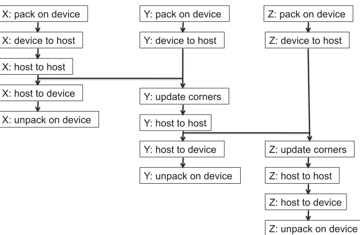
Figure 3: The dependency graph for the data packing and movement operations required within the communication stage of the application. The labels X, Y, and Z correspond to data transfers in each of the 3 spatial directions.
We use the same domain decomposition and message passing framework as the CPU version. Within each sub-domain (allocated to one MPI task) the GPU implementation proceeds as described in the Section 2.2. The only additional complication is that halo transfers between GPUs must be staged through the host. This means host MPI sends must be preceded by appropriate device to host transfers and host MPI receives must be followed by corresponding host to device transfers. In practice, this data movement requires additional GPU kernels to pack and unpack the relevant data before and after corresponding MPI calls. The CPU version uses MPI datatype functionality to designate the lattice sites, and velocity components within each lattice site, that are required for a specific direction of transfer (i.e. the complexities in buffer packing are handled by the MPI library). The lack of MPI functionality in the GPU memory space means that this filtering had to be done by hand in the abovementioned CUDA buffer-packing kernels.1
The standard shift algorithm, in which each co-ordinate direction is treated in turn, does provide some scope for the overlapping of different operations, as can be seen by the dependency graph in Figure 3. For example, after the data for the first co-ordinate direction have been retrieved by the host, these can be exchanged using MPI between hosts at the same time as kernels for packing and retrieving of data for the second co-ordinate direction are executed. This overlapping must respect the synchronisation required to ensure that data
1 At the time of writing, CUDA-aware MPI implementations that potentially
simplify the situation are becoming available, but still lack maturity. The Cray implementation on Titan does not yet support the MPI-datatype functionality used in the CPU version of Ludwig. When possible, we will compare performance with our hand-written inter-GPU communication code.
Overlapping(within(CommunicaFon(Phase(
11
X: pack on device X: device to host X: host to host X: host to device X: unpack on device
Y: update corners Y: pack on device Y: device to host
Y: host to host
Z: pack on device Z: device to host
Z: host to host Y: host to device
Y: unpack on device
Z: host to device Z: unpack on device Z: update corners
values at the corners of the sub-domain are transferred correctly. We use a separate CUDA stream for each co-ordinate direction (i.e. each of the three X, Y and Z columns of operations shown in Figure 3): this allows some of the host-device communication time to be effectively “hidden” behind the host-host MPI communication, resulting in an overall speedup. The effect of this overlapping optimisation is measured in the following section.
3
Results and Discussion
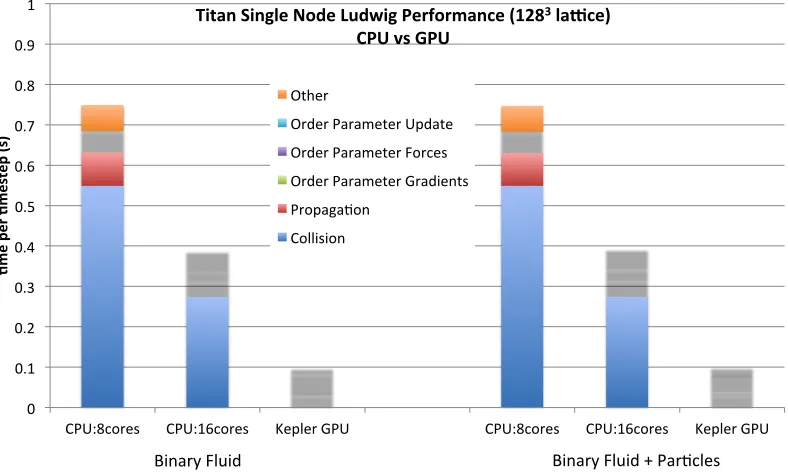
[image:10.595.95.489.477.713.2]The Cray XK7 Titan machine at Oak Ridge National Laboratory comprises 18,688 nodes, each with a single NVIDIA K20X (Kepler) GPU augmenting an AMD Opteron 6274 16-core CPU, where the nodes are connected via the Cray Gemini network [24]. In Figure 4 we compare the computational time of the CPU and GPU versions of Ludwig, for the binary fluid system, within a single node of Titan (i.e. one CPU is compared to one GPU). We plot the time per timestep with and without the inclusion of colloidal particles. For the latter we include 30 particles, corresponding to a volume fraction of around 0.1%. This is relatively low compared to typical simulations that would require 1-10%, but it is sufficient to analyse whether our general mechanisms for handling particles have incurred significant overhead. We decompose results into the different stages in the calculation. For the CPU version, we include results both fully populating and half populating each chip with MPI tasks (since the latter can potentially be beneficial in some cases): the fully populated results for which all 16 cores are utilised clearly has the advantage.
Figure 4: The time taken for the binary fluid system on a single node. Results are shown with and without the inclusion of colloidal particles. The results using a single AMD Interlagos 16-core CPU (either fully or half populated) are compared to those using a single NVIDIA Kepler GPU. All results are decomposed into the different stages within the computation.
0" 0.1" 0.2" 0.3" 0.4" 0.5" 0.6" 0.7" 0.8" 0.9" 1"
CPU:8cores" CPU:16cores" Kepler"GPU" CPU:8cores" CPU:16cores" Kepler"GPU"
!me$p
er$!mes
tep
$(s
)$
Titan$Single$Node$Ludwig$Performance$(1283$la?ce)$ CPU$vs$GPU$
Other"
Order"Parameter"Update" Order"Parameter"Forces" Order"Parameter"Gradients" PropagaDon"
Collision"
It can be seen that, for the non-particle case, the GPU performs the calculation around a factor of 4 faster than the (fully-populated) CPU. The picture is very similar when colloidal particles are included into the binary fluid, indicating that we have successfully implemented this functionality without discernible overheads. It can be seen that all the computational components of the calculation have been successfully accelerated on the GPU, with the exception of the calculation of the order parameter gradients. This memory-bandwidth intensive code section is performing better on the CPU, perhaps taking advantage of the caching architecture, and further effort is required to improve this part of the code in the GPU version.
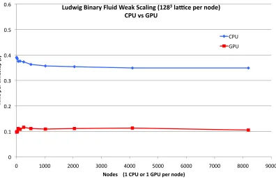
Figure 5: The dependence of runtime on the number of nodes utilised, where the problem size increases with the number of nodes. Diamonds denote use of a single 16-core AMD Interlagos CPU per node, and squares denote use of a single NVIDIA Kepler GPU per node.
In Figure 5 we extend the results for the non-particle case to multiple nodes, noting that the particle case uses the same communication mechanism. We keep the problem size per node fixed, i.e. measure weak scaling, where the time taken per timestep would stay constant in the ideal case. We plot against the number of nodes, i.e the number of GPUs or (fully populated) 16-core CPUs. It can be seen that the GPU code scales perfectly up to the largest size available at the time of writing, 8192 GPUs. The CPU code actually super-scales at low node-counts. This may be attributable to the MPI tasks within each node becoming out of synchronisation leading to less memory bandwidth contention. The performance advantage of the GPU version ranges from a around factor of 4 at low node counts to around a factor of 3.5 at high node counts.
!" !#$" !#%" !#&" !#'" !#(" !#)"
!" $!!!" %!!!" &!!!" '!!!" (!!!" )!!!" *!!!" +!!!" ,!!!"
!"
#$%&
$'%(#$)
*$&
%+),
%
-./$)%%%%+0%123%.'%0%423%&$'%5./$,%
67/8"9%:"5;'<%=>7"/%?$;@%AB;>"59%+0CDE%>;FB$%&$'%5./$,%%
123%G)%423%%
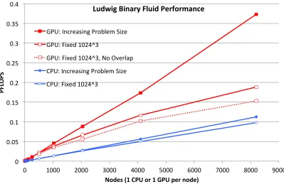
Figure 6: The dependence of performance, in PFLOPS, on the number of nodes utilised. For closed symbols, the problem size increases with the number of nodes (i.e. weak scaling). For open symbols, the problem size is fixed (such that that it matches the weak scaling case at 512 nodes). Diamonds denote use of a single 16-core AMD Interlagos CPU per node, and squares denote use of a single NVIDIA Kepler GPU per node. The series represented by the dashed line shows results when communication overlapping is disabled.
In Figure 6 we translate these results into raw performance in PFLOPS, inferred from the timings using a baseline performance measurement taken using the CrayPAT tool on the CPU version on a single node. Overall performance is reflected by the gradients, and scaling reflected by closeness to linearity, of the series: curvature indicates deviation from ideal scaling. We also include strong scaling results, where the problem size is fixed whilst the number of nodes varies. We choose a size of 10243 (which matches that used at 512 nodes in the
weak scaling analysis) since this is roughly similar to the size required for current research.
It can be seen that the benchmark does exhibit strong scaling up to the largest node count, in the sense that the performance continues to improve. However the parallel efficiency clearly reduces as the node count increases. We include the results gained when the communication overlapping optimisation described in the previous section is disabled (dotted line). It can clearly be seen that the overlapping has a significant effect in improving the strong scaling.
Profiling analysis indicates that the deviation from ideal strong scaling can be attributed to two factors. The first is that, as the number of nodes increases, the domain size per node decreases, and each GPU becomes underutilised reducing the computational performance. For the more computationally demanding liquid crystal case, the strong scaling may therefore be better: this is yet to be measured. The second factor is simply that the communication costs increase as the number of nodes increases. Future work will attempt to address this by
0" 0.05" 0.1" 0.15" 0.2" 0.25" 0.3" 0.35" 0.4"
0" 1000" 2000" 3000" 4000" 5000" 6000" 7000" 8000" 9000"
PFL
O
PS
&
Nodes&(1&CPU&or&1&GPU&per&node)&
Ludwig&Binary&Fluid&Performance&&&&
GPU:"Increasing"Problem"Size" GPU:"Fixed"1024^3"
overlapping the communication stage of the timestep with an appropriate computational kernel. One option is to split one or more of the lattice based kernels into two factors: one which processes the edges of the (sub-)domain, and the other the interior. It should then become possible to overlap the interior kernel, which has no dependency on halo data, with the communication stage.
Conclusions
We have described the steps take to augment the Ludwig code with functionality required for efficient utilisation of GPU-accelerated architectures, for the simulation of complex fluids. We have added the necessary functionality using NVIDIA CUDA in a maintainable fashion, and we discussed the tuning required to optimally exploit each GPU, such that it operates several times faster than a (optimally utilised) CPU. For the intricate problem of moving solid particles, we find it is possible to retain the more serial elements related to particle link operations on the CPU, while offloading only the parallel lattice-based operations involving the LB distribution to the GPU, minimising host-device movement of data. By retaining domain decomposition and message passing via MPI, we have demonstrated it is possible to scale complex fluid problems to large numbers of GPUs in parallel, through careful minimisation of the overheads associated with communications: we demonstrated excellent weak scaling using up to 8192 GPUs. When we fix the problem size at that required for current research, we find that we can reasonably use in the region of 512-2048 GPUs while retaining good parallel efficiency.
Future work is required in further improving both strong scaling and maintainability. To address the first issue, there is scope to overlap communication with computation to hide overheads. Related to this, the introduction of autotuning techniques may help to find the most optimal configuration out of the multitude of choices in ordering, overlapping, decomposing etc. that arise with complex applications on complex hardware. From a software engineering viewpoint, some duplication of code to allow efficient implementation on both host and device is currently required. This issue might be addressed by approaches such as automatic kernel generation, but may also be addressed naturally in time as GPU and CPU hardware converge.
Acknowledgements
Bibliography
[1] Desplat, J.-C., I. Pagonabarraga, and P. Bladon. LUDWIG: A parallel lattice-Boltzmann code for complex fluids. Comput. Phys. Comms. 134 273, (2001)
[2] O. Henrich, K. Stratford, D. Marenduzzo, P. V. Coveney, M. E. Cates. Rheology of Lamellar Liquid Crystals in Two and Three Dimensions: A Simulation Study. Soft Matter 8 (14), 3817-3831 (2012)
[3] O. Henrich, K. Stratford, D. Marenduzzo, P. V. Coveney, M. E. Cates. Confined Cubic Blue Phases under Shear. J. Phys. Condens. Matter (2012) [4] O. Henrich, K. Stratford, M. E. Cates, D. Marenduzzo. On the structure of
blue phase III. Phys. Rev. Lett. 106, 107801 (2011)
[5] X. Wei, W. Li, K. Muller, and A.E. Kaufman. The lattice Boltzmann method for simulating gaseous phenomena. IEEE Transactions on Visualization and Computer Graphics 10, 164--176 (2004)
[6] H. Zhu, X. Liu, Y. Liu, and E. Wu. Simulation of miscible binary mixtures based on lattice Boltzmann method. Comp. Anim. Virtual Worlds 17, 403--410 (2006)
[7] Y. Zhao. Lattice Boltzmann based PDE solver on the GPU,Visual Comput., doi 10.1007/s00371-0070191-y (2007)
[8] Tolke. Implementation of a lattice Boltzmann kernel using the compute unified device architecture developed by nVIDIA, Comput. Visual Sci. 13
29--39 (2010)
[9] Z. Fan, F. Qiu, A. Kaufman, and S. Yoakum-Stover. GPU cluster for high performance computing. Proceedings of ACM/IEEE Supercomputing Conference, pp. 47--59, IEEE Computer Society Press, Pittsburgh, PA (2004)
[10] J. Myre, S.D.C. Walsh, D. Lilja, and M.O. Saar. Performance analysis of single-phase, multiphase, and multicomponent lattice Boltzmann fluid flow simulations on GPU clusters. Concurrency Computat. Pract. Exper.
23, 332--350 (2011)
[11] C. Obrecht, F. Kuznik, B. Tourancheau, and J.-J. Roux. Multi-GPU implementation of the lattice Boltzmann method. Comput. Math. with Applications, doi:10.1016/j.camwa.2011.02.020 (2011)
[12] M. Bernaschi, M. Fatica, S. Melchionna, S. Succi, and E. Kaxiras. A flexible high-performance lattice Boltzmann GPU code for the simulations of fluid flow in complex geometries. Concurrency Computat.: Pract. Exper., 22, 1--14 (2010)
[13] W. Xian and A. Takayuki. Multi-GPU performance of incompressible flow computation by lattice Boltzmann method on GPU cluster. Parallel Comput., doi:10.1016/j.parco.2011.02.007 (2011).
[14] C. Feichtinger, J. Habich, H. Kostler, G. Hager, U. Rude, and G. Wellein. A flexible patch-based lattice Boltzmann parallelization approach for heterogeneous GPU-CPU clusters. Parallel Comput. 37 536--549 (2011) [15] S.D.C. Walsh and M.O. Saar. Developing extensible lattice Boltzmann
[16] S. Williams, L. Oliker, J. Carter, and J Shalf. Extracting ultra-scale lattice Boltzmann performance via hierarchical and distributed auto-tuning, Proc. SC2011 (2011)
[17] C.K. Aidun and J.R. Clausen. Lattice Boltzmann method for complex flows. Ann. Rev. Fluid Mech. 42 439--472 (2010)
[18] K. Stratford, R. Adhikari, I. Pagonabarraga, and J.-C. Desplat. Lattice Boltzmann for Binary Fluids with Suspended Colloids. J. Stat. Phys. 121, 163 (2005)
[19] A.J. Bray. Theory of phase-ordering kinetics. Adv. Phys. 43 357—459 (1994).
[20] V.M. Kendon, M.E. Cates, I. Pangonabarraga, J.-C. Desplat, and P. Bladon. Inertial effects in three-dimensional spinodal decomposition of a symmetric binary fluid mixture: a lattice Boltzmann study. J. Fluid Mech.,
440, 147--203 (2001)
[21] D. Marenduzzo, E. Orlandini, M.E. Cates, J.M. Yeomans. Steady-state hydrodynamic instabilities of active liquid crystals: Hybrid lattice Boltzmann simulation, Physical Review E 76, 031921 (2007)
[22] A.J.C. Ladd. Numerical simulations of particle suspensions via a discretized Boltzmann equation. Part 1. Theoretical foundation, J. Fluid Mech. 271 285--309 (1994); Part II. Numerical results, ibid. 271 311--339 (1994)
[23] N.-Q. Nguyen and A.J.C. Ladd. Lubrication corrections for lattice Boltzmann simulations of particle suspensions. Phys. Rev. E 66 046708 (2002)