Multi-population adapative inflationary differential evolution

INFLATIONARY DIFFERENTIAL

EVOLUTION

Marilena Di Carlo

Mechanical and Aerospace Engineering

University of Strathclyde, Glasgow, United Kingdom

[email protected]

Massimiliano Vasile

Mechanical and Aerospace Engineering

University of Strathclyde, Glasgow, United Kingdom

[email protected]

Edmondo Minisci

Mechanical and Aerospace Engineering

University of Strathclyde, Glasgow, United Kingdom

[email protected]

Abstract In this paper, a multi-population version of Adaptive Inflationary Differ-ential Evolution, which automatically adapts the crossover probability and the differential weight of the Differential Evolution, is presented. The multi-population algorithm exploits the use of different popula-tions, and the local minima found by each population, to assess the distance between minima; a probabilistic kernel based approach is then used to automatically adapt the dimension of a bubble in which the population is re-initialized after converging to a local minimum. The algorithm is tested on two real case functions and on two difficult aca-demic functions.

Keywords: Adaptive algorithms, Differential evolution, Global optimization.

1.

Introduction

Differential Evolution (DE), [13], is a population-based stochastic al-gorithm for solving optimization problems. Although it has proved to be a very efficient global optimizer, work has been done to enhance its performance by combining it with deterministic or stochastic opti-mizers [4, 5, 15]. In [19], Inflationary Differential Evolution Algorithm (IDEA) was introduced. IDEA is based on the hybridization of Differ-ential Evolution (DE) with the restarting procedure of Monotonic Basin Hopping (MBH) algorithm [20]. The performance of IDEA was found to be dependent upon the parameters controlling both the DE and MBH heuristics [19]. In particular, the DE performance is strongly influenced by the crossover probability, CR, and the differential weight, F, whose best settings are heavily problem dependent [8].

The need to have an algorithm capable of self-adapting these two parameters has resulted in many works [1, 3, 10, 12, 14]. The next step in the development of IDEA has therefore been the adaptation of CR

andF, leading to Adaptive Inflationary Differential Evolution Algorithm (AIDEA) [11]. This algorithm uses a probabilistic kernel based approach to automatically adapt the values of both CR and F.

Starting from the successful results of AIDEA, this paper introduces a multi-population version of AIDEA (MP-AIDEA), using different strate-gies to create the mutant vector of the DE, different stratestrate-gies to adapt

CR and F and a new mechanism to adapt the dimension of the search space in which the population is re-initialized. Other multi-populations DE algorithms have been presented in [16, 21, 22].

In the first part of this paper MP-AIDEA is described. Then the results of four test cases are presented.

2.

Multi-Population Adaptive Inflationary

Differential Evolution Algorithm

The algorithm presented in this paper is a further development of AIDEA [11]. In the following, a summary of AIDEA and a detailed description of MP-AIDEA are given.

AIDEA. The first step in the run of AIDEA is a DE process in which each element of the population is associated to a different value ofCR

The found local minimum is archived in a matrix of minima and the population is restarted in a bubble of dimension δlocal around the local

minimum (local restart). Local restart is iterated up to a predefined maximum value, identified by the valueiun. When this value is reached the population is restarted at a distanceδglobal from the cluster of local minima found thus far (global restart). The algorithm stops when the maximum number of function evaluation is reached.

MP-AIDEA. In MP-AIDEA the single population of AIDEA is

re-placed by many populations. The common archive of local minima of all the populations can be used to create the mutant vector of the DE. Three strategies have been considered for the generation of the mutant vector: 1) DE/best/1-DE/rand/1: the mutant vector is created ran-domly using the best element or a random element of the population; 2)

DE/arch/1-DE/rand/1: the mutant vector is created randomly using an element from the archive of local minima or a random element of the population: 3) DE/arch/1-DE/best/1: the mutant vector is created randomly using an element from the archive of local minima or the best element of the population.

As regards the adaptation, the presence of many populations can be exploited to adaptCR andF in a different way with respect to AIDEA. Two strategies for the adaptation of CR and F are proposed: 1) MP-AIDEA-CRF1 (CR and F adaptivity realized using CR and F values equal for every element of each population and comparing the popula-tions to each other) and 2) MP-AIDEA-CRF2 (CR and F adaptivity realized using differentCRand F values for each element of each popu-lation and comparing elements of each single popupopu-lation to each other, as in AIDEA [11]).

Finally, a strategy is proposed to adapt also the dimension of the bub-ble for the local restart of the population, using a kernel based approach similar to the one used for the adaptation ofCRandF. Considering all these possibilities, twelve different versions of the algorithm have been developed and tested:

- MP-AIDEA 1: MP-AIDEA-CRF1-DE/best/1-DE/rand/1

- MP-AIDEA 2: MP-AIDEA-CRF1-DE/arch/1-DE/rand/1

- MP-AIDEA 3: MP-AIDEA-CRF1-DE/arch/1-DE/best/1

(number of elements in each population),Npop(number of populations),

iun(maximum number of local restart), ¯ρ(size of the convergence box),

δglobal (distance from the cluster centres for the global restart) andδlocal

(dimension of the bubble for the local restart, if not adapted) as in line 1 and initializing the populations (line 3). The joint PDF for CR and

F is then initialised to be a uniform distribution (lines 4 and 5). For MP-AIDEA-CRF1, DE is run (line 11) drawing probabilistically a value for F and CR from CRF for each population (line 9) and CRF is updated on the basis of the improvement of the populations (step 15). For MP-AIDEA-CRF2, lines 9, 15 and 16 are to be considered inside theforcycle over the elements of the population (different values ofCR

andF for each element of the populations). If the populations contracts below a predefined threshold (step 18), a local optimizer is run from the current minimum (line 19) and the found local minimum is saved in an archive of local minima of all the populations (line 32). iunm is updated based on the improvement of the value of fmin,m (lines 23 to

28). If the adaptation of δlocal is performed, when all the population have performed the local search, a matrix B for the adaptation of the dimension of the bubble can be created (step 34, Algorithm 3) using the local minima found thus far. At this point the populations go through local or global restart according to lines 39 to 45. In particular, if the local optimizer failed to improve the value of fmin more than iunmax

times, the population is restarted globally andiunis set to 0, otherwise the population is restarted within a local bubble andiun=iun+ 1. The dimension of the bubble for the local restart is sampled from matrixB

(line 40) or is the one defined at line 1 if δlocal is not adapted. The adaptation ofB(line 36) is done only when the local optimizer has been applied to all the population for the second time (for each population, the adaptation can be performed only if two local minima are known for that population). At this point, the loop restart from the initialization of CRF. As a terminal criterion the algorithms stops if the maximum number of function evalutation nf eval,max has been reached.

CR and F adaptation. The updating procedure for CRFis

de-tailed in Algorithm 2 for MP-AIDEA-CRF1. For each population, the maximum objective function difference between parents and children,

sub-stitutesCRFj,1 (line 7) only ifddmax is greater than a given valueCRC (line 6), [11].

For MP-AIDEA-CRF2 the for cycle in line 2 is substituted by afor

cycle over the elements of the single population and ddmax is replaced byf(xi,k)−f(xi,k+2) for each elementiof the population, as in [11].

δ adaptation. The generation of the matrix B for the adaptation of the dimension of the bubble for the local restart is described in Algo-rithm 3; it reflects the procedure for the creation ofCRFand is based on the computation of the distance between the local minima found by the different populations and stored in the common archive of local minima. The updating procedure forB, detailed in Algorithm 4, follows the same approach used for the adaptation of CRF; the distance between local minimum found at subsequent local restart is used to assess the validity of the used dimension of the bubble for the local restart (a local restart is effective if the algorithm move from a local minimum to another).

The process of adaptation of the dimension of the bubble for the local restart will be presented in greater details in the first two test cases of the Test Results section.

3.

Test Results

The test cases are taken from the technical report of the CEC 2005 and CEC 2011 competitions [6,17]. The considered problems are: Spread Spectrum Radar Polyphase Code Design and Tersoff Radar Function Minimization Problem from CEC 2011; Schwefel’s Problem, Function 12, and Rotated Version of Hybrid Composition Function, Function 16, from CEC 2005. The statistics reported are computed on the results obtained from 100 independent runs in which new populations are generated at each run. The success rate reported in the next tables and figures is computed as number of times (over the 100 runs) in which the minimum found by the algorithm is lower thanfmin+ǫwherefmin is the minimum value of the function and ǫ is a given threshold [18]. ǫ= 0.001 for the test cases from CEC 2011 andǫ= 0.01 for the CEC 2005 problems [17].

3.1 Spread Spectrum Radar Polyphase Code Design

This problem has dimension nD = 20 and the best solution found is fmin = 0.5. The maximum number of function evaluation is 1.5e5 [6]. The same parameters setting of [11] was used, that is δlocal = δglobal =

Algorithm 1 Multi-Population Adaptive Inflationary Differental Evo-lution Algorithm

1: Set values fornpop,Npop,iun, ¯ρ,δglobal

2: Setnf eval,m= 0 andkm= 1 for all populationsm∈[1, . . . , Npop]

3: Initialize populationx_m,i,kfor allm∈[1, . . . , Npop] and for alli∈[1, . . . , npop]

4: A regular mesh with (nD+ 1)2points (wherenD is the dimensionality of the problem) in the spaceCR∈[0.1,0.99]xF ∈[−0.5,1] is created

5: InitializeCRF with points of the mesh: CRF_j,1 ← CRj and CRFj,2 ←Fj for allj ∈ [1, . . . ,(nD+ 1)2]

6: Associate to each row ofCRF_{an elementddj= 0 for allj∈[1, . . . ,(nD+ 1)}2

]

7: Row sortCRF_{in terms ofddvalues}

8: for_{m∈[1, . . . , Npop]}do

9: SampleCR_m,kandF_m,kfromCRF

10: for_{i∈[1, . . . , npop]}do

11: x_{m,i,k+1←DE(}x_m,i,k,CR_m,k,F_m,k)

12: nf eval,m=nf eval,m+ 1

13: end for

14: km=km+ 1

15: UpdateCRF(see Algorithm 2)

16: Row sortCRFin terms ofddvalues

17: ρm= max (||xm,i,k−xm,j,k||) ∀xm,i,k,xm,j,k∈Pm,k

18: if_ρm< ρ¯·ρmax,m then

19: Run a local optimizer fromx_best,m and letx_l,mbe the local minimum found by the local optimizer

20: if_f(x_l,m)< f(x_best,m) then

21: f(x_best,m)←f(x_l,m)

22: end if

23: iff(x_best,m)< fmin,mthen

24: fmin,m←f(xbest,m)

25: iunm= 0

26: else

27: iunm=iunm+ 1

28: end if

29: else

30: Termination_{Unlessnf eval,m≥nf eval,maxgoto (10)}

31: end if

32: Addx_{best,mto the archive of minima of population: Ag,m=Ag,m+{}x_best,m}

33: end for

34: Create matrixBfor adaptation of the dimension of the bubble (see Algorithm 3)

35: if_{(All population went for the 2nd time through the local minimizer)}then

36: UpdateB(see Algorithm 4)

37: end if

38: for_m∈[1, . . . , Npop]do

39: if_iun≤iunmaxthen

40: Sampleδlocal,mfromBto define the bubbleDm

41: Initialize populationx_m,i,kfor alli∈[1, . . . , npop] in the bubbleDm

42: else

43: Define clusters in the archive and compute baricentrex_c,m of each cluster

44: Initialize populationx_m,i,kfor alli∈[1, . . . , npop] such that∀i, j||xm,i,k−xm,j,k||>

δglobal

45: end if

46: end for

47: Termination_{Unlessnf eval,m≥nf eval,max goto (4)}

Table 1, along with the results of two of the best performing algorithms of the CEC 2011 competition, the Genetic Algorithm with Multi Parent Crossover (GA-MPC) [7] and the Weed Inspired Differential Evolution (WI-DE) [9].

Algorithm 2Updating procedure for CRF

1: For each population compute ddmax,m = max||f(xm,i,k+1) −

f(xm,i,k)||for all i∈[1, . . . , npop]

2: for m_∈[1, . . . , Npop]do

3: forj ∈[1, . . . ,(nD+ 1)2] do

4: if ddj < ddmax,m then

5: CRFj,2,k←Fm,k

6: if ddmax,m> CRC then

7: CRFj,1,k ←CRm,k

8: end if

9: end if

10: end for

11: end for

Algorithm 3Generation of matrix Bfor the adaptation of the bubble 1: Compute mean and minimum distance between all local minima in

Agm for allm∈[1, . . . , Npop]: dminM IN and dminM EAN

2: Create regular mesh with (nD + 1)2 points in the space [dminM IN,dminM EAN]

3: Initialize B with points of the mesh

4: Associate to each row of B an element ddbj = 0 for all j _∈

[1, . . . ,(nD+ 1)2]

5: Row sort B in terms ofddb values

Algorithm 4Updating procedure for B

1: For each population compute pm=||xl,m,k+1−xl,m,k||

2: for m∈[1, . . . , Npop]do

3: forj _∈[1, . . . ,(nD+ 1)2_{] do} 4: if ddbj< pm then 5: Bj,1,k ←δlocal,m

6: end if

7: end for

8: end for

Table 1. Spread Spectrum Radar Polyphase Code Design – AIDEA, GA-MPC and WI-DE results.

Algorithm npop Min Mean Max Str.Dev. S.Rate

AIDEADE/best 20 0.5000 0.5150 0.6509 0.0343 -AIDEA DE/best-DE/rand 20 0.5000 0.5130 0.6422 0.0263 75

GA-MPC - 0.5000 0.7484 0.9334 0.1249

-WI-DE - 0.5000 0.656 0.993 0.116

-2 4 6 8 10 12 14 16 18 20 22 0

20 40 60 80 100

N

pop

Success rate

MP−AIDEA DE/best−DE/rand

AIDEA MP−AIDEA 1 MP−AIDEA 4 MP−AIDEA 7 MP−AIDEA 10

2 4 6 8 10 12 14 16 18 20 22 0

20 40 60 80 100

N

pop

Success rate

MP−AIDEA DE/arch−DE/rand

AIDEA MP−AIDEA 2 MP−AIDEA 5 MP−AIDEA 8 MP−AIDEA 11

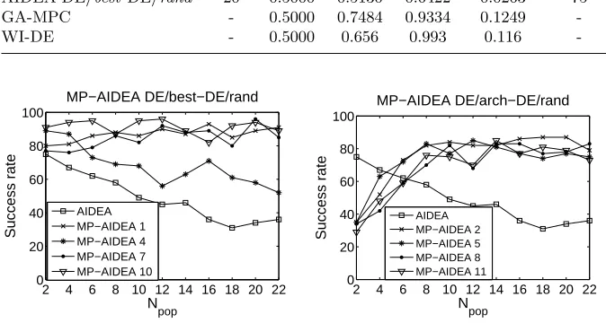
Figure 1. Spread Spectrum Radar Polyphase Code Design – MP-AIDEA success rate.

rate increasing with Npop and greater than the success rate of AIDEA

forNpop sufficiently high.

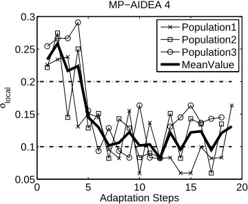
In Figure 2 the process of adaptation of the dimension of the bubble for the local restart is shown for MP-AIDEA 4 and Npop = 3 for a sequence of 19 subsequent local restarts before the global restart of the algorithm. The bold line represents the mean value ofδlocal over all the populations. It is evident thatδlocal = 0.1 proves to be a good guess for the value of δlocal.

3.2 Tersoff Potential Function Minimization Problem

This problem has dimensionnD = 30 and the best solution isfmin =

−36.9286. The maximum number of function evaluation is 1.5e5. AIDEA and MP-AIDEA were tested using two different sets of parameters set-tings: δlocal =δglobal = 0.1, ρ = 0.2, iun= 10 (Case 1) and δlocal = 0.3,

δglobal = 0.1, ρ = 0.2, iun = 10 (Case 2). The results obtained using

0 5 10 15 20 0.05

0.1 0.15 0.2 0.25 0.3

Adaptation Steps

δ local

MP−AIDEA 4

Population1 Population2 Population3 MeanValue

Figure 2. Spread Spectrum Radar Polyphase Code Design – adaptation ofδlocal.

Table 2. Tersoff Potential Function Minimization Problem – AIDEA, GA-MPC and WI-DE results.

Algorithm npop Min Mean Max Str.Dev. S.Rate

Case 1

AIDEA DE/best 20 -36.9286 -36.8527 -35.5171 0.2442 -AIDEA DE/best-rand 20 -36.9286 -36.8046 -35.9700 0.2483 34

Case 2

AIDEA DE/best-rand 20 -36.9286 -36.6219 -35.4467 0.4694 11

GA-MPC - -36.8457 -35.03883 -34.1076 0.8329

-WI-DE - -36.8 -35.6 -34.2 0.904

-In Figure 3 the results obtained from different combinations ofNpop×

npopare shown for the best variants of MP-AIDEA and for both Case 1 and Case 2.

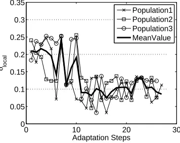
For Case 1 the best results are given by AIDEA 1 and MP-AIDEA 7. Changing the values ofδlocal from 0.1 to 0.3 (Case 2) results however in a successful performance of the algorithms with adaptation of δlocal, that is MP-AIDEA 4 and MP-AIDEA 10. This is due to the

fact that for Case 1 the chosen value of δlocal was close to the optimal value for this problem. This is proved in Figure 4, where the process of adaptation of δlocal is shown for MP-AIDEA 4 using 3 populations. Arbitrary chosen values, such asδlocal= 0.3 (Case 2) are very dissimilar

2x100 4x10 6x10 8x10 10 20 30 40 50 60 70 N

popxnpop

Success rate

Case 1 AIDEA MP−AIDEA 1 MP−AIDEA 4 MP−AIDEA 7 MP−AIDEA 10

2x100 4x10 6x10 8x10 10 20 30 40 50 60 70

N_popxn_pop

Success rate Case 2 AIDEA MP−AIDEA 1 MP−AIDEA 4 MP−AIDEA 7 MP−AIDEA 10

Figure 3. Tersoff Potential Function Minimization Problem – MP-AIDEA success rate.

0 10 20 30

0 0.05 0.1 0.15 0.2 0.25 0.3 0.35 Adaptation Steps δ local Population1 Population2 Population3 MeanValue

Figure 4. Tersoff Potential Function Minimization Problem – adaptation ofδlocal.

3.3 Schwefel’s Problem

Schwefel’s problem was tested with dimensionnD = 30 and nD = 50. The best solution is fmin = ₋460; the parameters settings is δlocal = δglobal = 0.1, ρ = 0.2 and iun = 5. The maximum number of function evalutions is 3e5 for the 30D problem and 5e5 for the 50D problem, [17]. The results obtained using AIDEA with DE strategy DE/rand/1 -DE/best/1 are reported in Table 3 as statistics of the objective function error values with respect to fmin, as required by [17], along with the

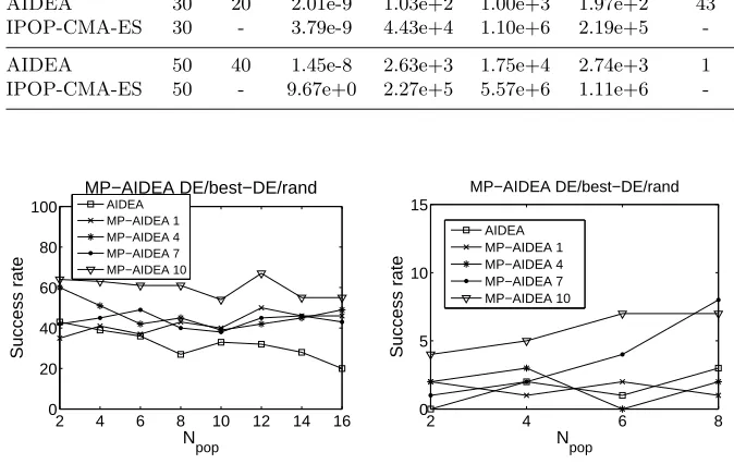
Table 3. Schwefel’s Problem – AIDEA and IPOP-CMA-ES results.

Algorithm nD npop Min Mean Max Str.Dev. S.Rate

AIDEA 30 20 2.01e-9 1.03e+2 1.00e+3 1.97e+2 43

IPOP-CMA-ES 30 - 3.79e-9 4.43e+4 1.10e+6 2.19e+5

-AIDEA 50 40 1.45e-8 2.63e+3 1.75e+4 2.74e+3 1

IPOP-CMA-ES 50 - 9.67e+0 2.27e+5 5.57e+6 1.11e+6

-2 4 6 8 10 12 14 16 0

20 40 60 80 100

N_pop

Success rate

MP−AIDEA DE/best−DE/rand

AIDEA MP−AIDEA 1 MP−AIDEA 4 MP−AIDEA 7 MP−AIDEA 10

2 4 6 8

0 5 10 15

N_pop

Success rate

MP−AIDEA DE/best−DE/rand

AIDEA MP−AIDEA 1 MP−AIDEA 4 MP−AIDEA 7 MP−AIDEA 10

Figure 5. Schwefel’s Problem – MP-AIDEA success rate.

In Figure 5 the success rates obtained for different values ofNpop, with

npop= 10 for the 30D problem and npop= 20 for the 50D problem, are shown for the most successful versions of MP-AIDEA. For the 30D prob-lem MP-AIDEA gives better results than AIDEA in most of the cases; for the 50D problem MP-AIDEA is able to find the global minimum of the function.

3.4 Rotated Version of Hybrid Composition

Function

For this function the best solution is fmin = 120, nD = 10, δlocal =

δglobal = 0.1, ρ = 0.2 and iun = 5. The maximum number of function evaluations is 1e5 [17]. The results obtained using AIDEA, IPOP-CMA-ES and MP-AIDEA are shown in Table 4 and Table 5, where results from different combinations ofNpop × npop are presented.

Table 4. Rotated Version of Hybrid Composition Function – AIDEA and IPOP-CMA-ES results.

Algorithm npop Min Mean Max Str.Dev. S.Rate

AIDEA 40 5.38e+1 1.02e+2 1.14e+2 8.42e+0 0

IPOP-CMA-ES - 7.92e+1 9.13e+1 9.68e+1 3.49e+0

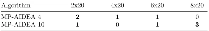
-Table 5. Rotated Version of Hybrid Composition Function – MP-AIDEA success rate.

Algorithm 2x20 4x20 6x20 8x20

MP-AIDEA 4 2 1 1 0

MP-AIDEA 10 1 0 1 3

4.

Conclusions

In this paper a multi-population version of AIDEA have been pre-sented and tested. Results have shown that MP-AIDEA can give results which are better, or at least comparable, to the ones provided by AIDEA. The new strategies DE/arch/1-DE/rand/1 and DE/arch/1-DE/best/1

have shown to be effective when the number of populations is not too low. The adaptation of the bubble dimension has proven to give good results, having moreover the advantage of not requiring the setting of the parameterδlocal for the dimension of the bubble of the local restart. In addition, the most successful versions of MP-AIDEA were able to locate for the first time the global minima of two difficult academic functions.

References

[1] M. M. Ali and A. Torn. Population set based global optimization algorithms: Some modifications and numerical studies. Comput. Oper. Res., 31(10):1703– 1725, 2004.

[2] A. Auger and N. Hansen. A Restart CMA Evolution Strategy with Increasing Population Size. Proc. IEEE Congress on Evolutionary Computation (CEC), pp. 1769–1776, 2005.

[3] J. Brest, S. Greiner, B. Boˇskovi´c, M. Mernik, and V. ˇZumer. Self-adapting control parameters in differential evolution: A comparative study on numeri-cal benchmark problem.IEEE T. Evolut. Comput., 10:646–657, 2006.

[5] L. Coelho and V. C. Mariani. A Hybrid Method of Differential Evolution and SQP for Solving the Economic Dispatch Problem with Valve-Point Effect. Ap-plications of Soft Computing, pages 311–320, 2006.

[6] S. Das, and P. N. Suganthan. Problem Definitions and Evaluation Criteria for CEC 2011 Competition on Testing Evolutionary Algorithms on Real World Optimization Problems. Technical Report, 2010.

[7] S. M. Elsayed, R. A. Sarker, and D. L. Essam. GA with a New Multi-Parent Crossover for Solving IEEE-CEC2011 Competition Problems. Proc. IEEE Congress on Evolutionary Computation (CEC), pp. 1034–1040, 2011.

[8] R. Gamperle, S.D. Muller, and P. Koumoutsakos. A Parameter Study for Dif-ferential Evolution. InProc. WSEAS International Conference on Advances in Intelligent Systems, Fuzzy Systems, Evolutionary Computation, pages 293–298, 2002.

[9] U. Halder, S. Das, D. Maity, A. Abraham, and P. Dasgupta. Self Adaptive Clus-ter Based and Weed Inspired Differential Evolution Algorithm for Real World Optimization.Proc. IEEE Congress on Evolutionary Computation (CEC), pp. 750–756, 2011.

[10] J. Liu and J. Lampinen. A fuzzy adaptive differential evolution algorithm.J. Soft Computing, 9:448–462, 2005.

[11] E. Minisci and M. Vasile. Adaptive Inflationary Differential Evolution. InProc. IEEE World Congress on Computational Intelligence (WCCI), 2014.

[12] M. G. H. Omran, A. Salman, and A. P. Engelbrecht. Self-adaptive Differential Evolution.Lect. Notes Artif. Intell., 3801:192–199, 2005.

[13] K. V. Price, R. M. Storn, and J. A. Lampinen.Differential Evolution. A Practical Approach to Global Optimization.Natural Computing Series, Springer, 2005.

[14] A. K. Qin, V. L. Huang, and P. N. Suganthan. Differential evolution algorithm with strategy adaptation for global numerical optimization. IEEE T. Evolut. Comput., 13:398–417, 2009.

[15] A. Qinq. Differential Evolution: Fundamentals and Applications in Electrical Engineering. John Wiley & Sons, 2009.

[16] D. Shen, Y. Li, B. Wei, and X. Xia. Adaptive Forking Multipopulation Differ-ential Evolution Algorithm for Multimodal Optimization.J. Convergence Infor-mation Technology, 7(5):218–227, 2011.

[17] P. N. Suganthan, N. Hansen, J. J. Liang, K. Deb, Y. P. Chen, A. Auger, and S. Tiwari. Problem Definitions and Evaluation Criteria for the CEC 2005 Special Session on Real-Parameter Optimization. Technical Report, 2005.

[18] M. Vasile, E. Minisci, and M. Locatelli. Analysis of Some Global Optimization Algorithms for Space Trajectory Design.J. Spacecraft Rockets, 47:334–344, 2010.

[19] M. Vasile, E. Minisci, and M. Locatelli. An Inflationary Differential Evolu-tion Algorithm for Space Trajectory OptimizaEvolu-tion. IEEE T. Evolut. Comput., 15:267–281, 2011.

[21] W. Yu and J. Zhang. Multi-population Differential Evolution with Adaptive Parameter Control for Global Optimization. In Proc. 13th Annual Conference on Genetic and Evolutionary Computation (GECCO), pages 1093–1098, 2011. [22] D. Zaharie. A Multipopulation Differential Evolution Algorithm for