SEQUENCING RELIABILITY GROWTH TASKS USING
MULTIATTRIBUTE UTILITY FUNCTIONS
KEVIN J WILSON∗, JOHN QUIGLEY Department of Management Science
University of Strathclyde, UK
In both hardware and software engineering, the reliability of systems improve over the Test, Analyse and Fix (TAAF) cycle as reliability tasks are performed and faults are designed out of the system. There are many possible tasks which could be carried out and a large numbers of sequences of these tasks possible. In this paper we consider the sequencing problem, taking into account the fact that the testing will be stopped once a reliability target is reached. We solve the problem by maximising the expectation of a two attribute utility function over cost and time on test. All marginal utilities are set to be risk averse. A reliability growth model based on the underlying engineering process is used. The method is illustrated with an example grounded in work with the aerospace industry.
Keywords: Reliability growth, utility, Bayesian, sequencing
1. Introduction
During new product development an initial design is subject to detailed anal-ysis, identifying improvements until performance requirements are met [1]. Common reliability tasks which analyse the design and subsequently facilitate the enhancement include Fault Tree Analysis (FTA), Failure Mode and Effects Analysis (FMEA), and Highly Accelerated Life Testing (HALT) [5]. These tasks can be resource intensive and costly to implement. Although each task assumes a different perspective upon the analysis of the design, the outcomes may not be mutually exclusive because each has the goal of design improve-ment by understanding weaknesses. Any weakness may be exposed through different routes. Therefore, the marginal benefit of introducing new analy-sis tasks to a development programme will eventually be outweighed by the marginal cost of implementing the analysis.
We have adapted a reliability model [6] to support the assessment of the system reliability. This point process model assumes a fixed but unknown
number of faults within the design and each is realised independently if the design is used on test or in-service. Dynamic reliability models have been considered previously by [8,2]. Prior distributions are elicited from engineers with to assess the design weaknesses and hence the number of potential faults that may exist, with uncertainty expressed through probability distributions. A discussion of the elicitation process is given in [3]. Historical data can be used to determine the expected rate of occurrence of faults.
In Section 2 we review the reliability model used in the paper. In Section 3 we outline a process to find the optimal sequence of tasks which maximises the prior expectation of a utility function over cost and time on test. In Section 4 we illustrative the method using an example. We then make some conclusions in the final section.
2. Optimal allocation of reliability tasks
2.1. Problem definition
We consider the model developed in [9,7]. Suppose that the current design of an engineering system has associated with it a number of identified engineer-ing concerns, labelled i = 1, . . . , I. Then, for each concern i, there is some probability, denoted λi, that this concern will ultimately be realised. Let us defineXi to be an indicator variable such that
Xi= (
1, if concerniis ultimately realised, 0, otherwise.
Then the probabilities ofXi being in its two possible states areλi and 1−λi respectively.
As part of the Test, Analyse And Fix (TAAF) cycle there are a number of possible tasks which could be performed on the equipment, labelled j = 1, . . . , J. Each of these tasks will have a certain efficacy at identifying each of the different faults in the system. Denote bypi,j the conditional probability that taskj will realise fault igiven that the fault truly exists.
We can elicit both λi and pi,j from engineering experts inside the organi-sation. If we assume that each time a fault is found and removed no new fault is added to the system, then in the system there will be some fixed unknown number of faults, denotedN.
2.1.1. Prior reliability
If we assume that the faults are independent then the reliability of the system at timet is given byR(t) =QIi=1Ri(t)Xi =QI
to performing any of the tasks the expected reliability is
EX[R(t)] = I Y
i=1
[1−(1−Ri(t))λi]
2.1.2. Post-development reliability
Suppose we have performed a number of the tasks. We will either observe fault iin one of the tests,di = 1, or not, di = 0. This will update, through Bayes Theorem, the probabilities of the faults truly existing to Pr(Xi= 1|di= 1) = 1,Pr(Xi= 0|di= 1) = 0, as when a fault is found it must exist and
Pr(Xi=xi|di = 0) =
1−λi
1−λi[1−QJj=1(1−pi,j)θj]
, xi= 0,
QJ
j=1(1−pi,j)
θjλ
i 1−λi[1−QJj=1(1−pi,j)θj]
, xi= 1,
where θj is an indicator variable which takes the value 1 if task j has been performed and 0 if not. The prior expectation of the reliability is then
ED
EX|D[R(t)] = I Y
i=1
1−(1−Ri(t))λi J Y
j=1
(1−pi,j)θj
.
3. Optimal sequencing of reliability tasks
3.1. Problem definition
We could perform all of the reliability growth tasks possible for a system. However, if we were to reach our reliability target after fewer than the allocated tasks, then we would stop testing and save time and money. Therefore, finding the optimal sequence of reliability tasks is an important question.
To model this we need to consider the probability distribution of the reli-ability as we are interested in quantities of the form Pr(R(t)≥R0) =α, for
someαclose to one. To do so let us transform the reliability so that it is not restricted to [0,1]. Specifically, define
η(t) = log [R(t)].
We can fully specify the distribution of the reliability by specifying m(t), v(t) as m(t) = EdEX|d[η(t)] and v(t) = Ed
EX|d
η(t)2 − Ed
EX|d[η(t)]
2
. These are calculated via
Ed
EX|d[η(t)n] = X
d I Y
i=1
Pr(Di=di) X
x I Y
i=1
Pr(Xi=xi|d)× " I
X
i=1
log (Ri(t)) #n
,
forn= 1,2.
These are not fast and efficient calculations to perform. Each vectordand xare of lengthI with each element having two possible states, 0 and 1. The number of sequences of lengthJisJP
J, whereP denotes permutations. There-fore the total number of calculations which would be necessary to evaluate the probability distribution ofη(t) for all sequences of lengthJisN = 22I+1×JP
J. For example, ifI= 5, J= 5 thenN = 245,760 and ifI= 15, J = 14 (still very small) thenN= 1.87×10²⁰. In practice, for a reasonably large problem, it is
not going to be possible to evaluate all of the required expectations exactly. We can approximate the logarithm of the reliability by taking a rare event approximation. If we do so we get
−log [R(t)] = I X
i=1
(1−Ri(t))λi− I X
i=1
(1−Ri(t))λi J X
j=1
θj(1−αi,j),
where αi,j is 1 if task j finds fault i given that faulti exists and 0 if it does not findiwhen it exists. In this case,
m(t) =−
I X
i=1
(1−Ri(t))λi− I X
i=1
(1−Ri(t))λi J X
j=1
θj(1−pi,j)
,
v(t) = I X
i=1
[(1−Ri(t))λi]
2
J X
j=1
θj(1−pi,j)pi,j.
By the Lyapanov Central Limit Theorem [4] the distribution of the approxi-mation is asymptotically Normal with increasing numbers of activities.
Using the approximations the total number of calculations required to solve the design problem for a sequence of lengthJ reduces toN = 2IJ×JP
J. In the specific cases, if I = 5, J = 5 thenN = 6000 and if I = 15, J = 14 then N = 3.66×10¹³. We see that the number of calculations required has been
3.2. Expected utility solution
We need to define a utility function which incorporates the uncertainty on the reliabilityR(t). The utility we define will include this reliability uncertainty in both the financial cost and time cost utilities and so there is no need to include a specific utility function for reliability. Thus the overall utility function will beU(Y, χ), whereY represents financial cost andχ represents time on test.
Suppose that all of the possible sequences of tasks of lengthJ are given by s1, . . . , sMJ, where MJ =
J PJ. Then the Bayesian optimal sequence of tasks is given by
max sMJ
Ed
EX|d[U(Y, χ)] ,
where the utility functionU(Y, χ) incorporates the probability distribution of R(t).
Suppose that we order the tasks for sequence si ascending from 1 to J. Then if we performj tasks the total costs and time on test will be given by yj(tot)=Pjk=1ykandχ
(tot)
j = Pj
k=1χk respectively. Introducing our rule that we stop testing if we reach the target reliability, the cost and time on test for sequencesi are
Y = J X
j=1
yj(tot)γj j−1
Y
k=1
(1−γj), χ= J X
j=1
χ(jtot)γj j−1
Y
k=1
(1−γj),
whereγj is an indicator variable which takes the value 1 ifR(t)> R0and 0 if
not. If we assume utility independence between cost and time on test we can then define the general utility function to be a binary node:
U(C) =p1U(Y) +p2U(χ) +p3U(Y)U(χ),
for trade-off parameters p1, p2, p3 such that p1+p2+p3 = 1. Examples of
suitable risk averse marginal utility functions for financial cost and time on test would be U(Y) = 1−(Y /Y0)2 and U(χ) = 1−(χ/χ0)2, however any
suitable functions on [0,1] could be used.
We see that, to calculate the expected utility of a particular sequence, we need E[γj], for all j, which are the Pr(R(t) > R0) for a particular stage of a
specific sequence.
4. Illustrative example
4.1. Background
could carry out to identify and design out these flaws. This means that in all there are 362,880 possible sequences of the tasks which could be carried out.
Each task has associated with it a cost of between 0 and 50 units and a duration of between 0 and 20 units. The target reliability, which would be assessed by the decision maker, is 0.8, the maximum time on test is 150 units and the maximum total cost, found by summing the costs of each of the possible tasks, is 258 units. We also require the marginal reliability functions for the faults. There are various possibilities here but if the rate of failure from the fault can be thought of as constant over time a suitable choice for the time to failure is the exponential distribution. This results in a marginal reliability function of
Ri(t) = exp{−µit},
where µi is the rate of failures resulting from fault i. The final parameters which need to be specified are the trade-off parameters for the binary utility function. In the example, theλi are between 0 and 0.5, 54% of the pi,j are equal to zero indicating that taskj will not find faultiand the rest are between 0 and 0.5 and eachµi is chosen to be 0.02.
4.2. Results
We wish to schedule the tasks in order to minimise the expected cost and total time on test. We do so by maximising the prior expected utility as outlined in the previous section. We have a single binary utility function for cost and time on test. Suppose that initially the decision maker felt that the utility of each was equally important. Thenp1= 1/2, p2= 1/2, p3= 0.
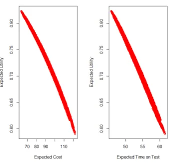
We calculate the expected utility for each and then choose the order with the maximum value. The expected utilities for all of the possible orderings are given against both expected cost and expected time on test in Figure 1.
We see that there are clear relationships between both cost and time on test and the expected utility, with the maximum utility achieved with low cost and low time on test. The relationship is stronger with cost than with time on test. The relationships reflect the quadratic forms of the marginal utility functions.
The optimal ordering of tasks has an expected utility of 0.875 and corre-sponds to the sequence (4,2,8,1,9,5,7,6,3). That is, we first carry out task 4 and then if we haven’t met the reliability target we move on to task 2. If we still haven’t met the reliability target we then carry out task 8, etc.
Figure 1. Expected utilities for the different task orderings against expected cost (left) and expected time on test (right).
Task 4 2 8 1 9 5 7 6 3
Cost 17 52 63 63 109 114 135 138 165
Time 9 10 18 24 40 43 48 52 67
Probability 0.0002 0.10 0.46 0.82 0.97 0.99 1.00 1.00 1.00
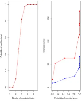
Plots of the probability of reaching the target after each task by the number of tasks completed (left) and the time and financial costs against the probability of reaching the target after each task (right) are given in Figure 2. In the right-hand plot financial costs are in red and time on test is in blue.
From the table and figures we see that it is not likely that we will have to perform all of the tasks to achieve the target reliability. It is likely that only 4 or 5 tasks will be needed and that we can reach the reliability target with a spend of 63-109 and a time on test of 24-40.
5. Summary
Figure 2. The probability of reaching the target reliability for a given number of tasks (left) and the financial cost (red) and time on test (blue) against the probability of reaching the target reliability (right).
References
[1] W. Blischke and D.N.P. Murthy.Reliability: Modelling, Prediction and Optimiza-tion. Wiley, 2000.
[2] D. P. Gaver. Random hazard in reliability problems. Technometrics, 5(2):211– 226, 1963.
[3] R. Hodge, M. Evans, J. Marshall, J. Quigley, and L. Walls. Eliciting engineering knowledge about reliability during design - lessons learnt from implementation. Quality and Reliability Engineering International, 17:169–179, 2001.
[4] K. Knight.Mathematical Statistics. Chapman and Hall, 2000. [5] P. O’Connor.Practical Reliability Engineering. Wiley, 2000.
[6] J. Quigley and L. Walls. Point process model for reliability analysis of evolu-tionary designs. Proceeding from MMR Conference, Trondheim, Norway, pages 551–554, 2002.
[7] J. Quigley and L. Walls. Trading reliability targets within a supply chain using Shapley’s value.Reliability Engineering and System Safety, 92:1448–1457, 2006. [8] Nozer D. Singpurwalla. Survival in dynamic environments.Statist. Sci., 10(1):86–
103, 02 1995.