Model-based controller design for a plastic film extrusion process

Hur, Sung-ho and Katebi, M.R. and Taylor, Andrew. Model-based controller design for a plastic film

extrusion process. In: IEEE Multi-Conference on Systems and Control (MSC), 8-10 September 2010,

Yokohama, Japan.

http://strathprints.strath.ac.uk/

27441

/

Strathprints is designed to allow users to access the research output of the University of

Strathclyde. Copyright © and Moral Rights for the papers on this site are retained by the

individual authors and/or other copyright owners. You may not engage in further

distribution of the material for any profitmaking activities or any commercial gain. You

may freely distribute both the url (

http://strathprints.strath.ac.uk

) and the content of this

paper for research or study, educational, or not-for-profit purposes without prior

permission or charge. You may freely distribute the url (

http://strathprints.strath.ac.uk

)

of the Strathprints website.

Model-based Controller Design for a Plastic Film Extrusion Process

Sung-ho Hur, Reza Katebi and Andrew Taylor

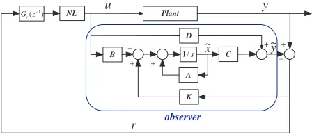
Abstract— This paper reports the development and imple-mentation of a model-based cross-directional controller for plastic film extrusion and other web-forming processes. The controller design has a similar structure to that of internal model control (IMC) with the addition of an observer whose gain is designed to minimise process and model mis-match. The observer gain is obtained by solving a multi-objective optimisation through the application of a genetic algorithm and simulation results are presented in this paper demonstrating improvements that can be achieved by the proposed controller over two existing CD controllers.

I. INTRODUCTION

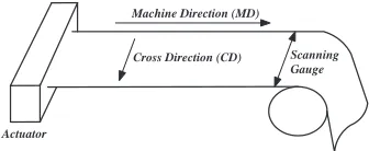
As with other web forming processes, such as the pa-permaking and metal-rolling, plastic film extrusion employs arrays of actuators across a continuously moving web to control the cross-directional (CD) profiles of key product properties. In plastic film, the main controlled property is finished product thickness profile as measured by a scanning gauge downstream from the actuators as illustrated in Fig. 1. The main stages of the plastic film extrusion process are extrusion, where a polymer melt is fed into a die; casting, where the polymer melt is discharged through the die gap onto a rotating casting drum to form a continuous amorphous sheet; machine-directional (MD) stretching; cross-directional (CD) stretching; heat setting; and winding, where finished product is rolled. The array of actuators is located at the die gap and the scanning gauge is placed prior to winding, hence there is a significant time lag between the two as shown in Fig. 1.

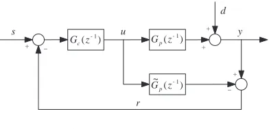
CD control has received a considerable attention in the control systems community and there have been many pa-pers published studying various CD controller designs – see [1] and references therein. In this paper, model-based CD controller design is presented and applied to a first-principles model of a plastic film extrusion process. This model is described in [2] and is used to simulate the plant throughout this paper. The proposed controller design has a similar structure to that of the controller reported in [3] since both are modifications to the internal model control (IMC), which can be regarded as a dynamic compensator (Fig. 3). Our controller design requires the solution of a quadratic programming problem online for optimal steady state performance. Model-based CD controllers require an accurate reference model and controller performance can therefore be improved by minimising the effects of process-model mismatch and disturbances. Consequently, the

pro-This work was supported by DuPont Teijin Films UK Ltd and UK EPSRC S. Hur and R. Katebi are with the Department of Electronic and Electrical Engineering, University of Strathclyde, [email protected]

A. Taylor is with DuPont Teijin Films UK Ltd

Machine Direction (MD)

Cross Direction (CD)

Actuator

Scanning Gauge

Fig. 1. Generic web forming process

posed controller design employs an observer in place of the reference model in order to reduce the effect of process-model mismatch as well as disturbances.

The observer design is presented in Section II along with the genetic algorithm [4] that solves the resulting multi-objective optimisation problem. The dynamic compensator is discussed in Section III and Section IV illustrates how the steady state performance is achieved by solving a quadratic programming problem [3], [5]. The computational struc-ture of the controller is summarised in Section V, and the implementation and performance of the controller are demonstrated in Section VI followed by a conclusion in Section VII.

II. OBSERVER DESIGN

Plant

u y

NL

) (_z-1

Gc

B 1/s C

A +

observer

K

r

+ +

_

+ +

D

+ +

x

~ ~_y

Fig. 2. Proposed controller

The mathematical description of the observer is as follows:

˙˜

x(t) =A˜x(t) +Bu(t) +K(y(t)−˜y(t)) = (A−KC)˜x(t) + (B−KD)u(t) +Ky(t) ˜

y(t) =C˜x(t) +Du(t) (1)

where y(t) ∈ _Rn _{and ˜y(t) ∈}

Rn denote the plant

mea-surements and model estimates, respectively, andu(t)∈Rm

represents the control action. The term involving the observer gain K should correct the observer estimate continuously such that˜y(t)follows y(t)more closely. This consequently means that the effects of process-model mismatch and dis-turbances can be reduced by optimisingK. Derivation of an optimal gainKis summarised in this section. Gc(z−1) and

N Lin Fig. 2 are responsible for dynamic compensation and steady state performance respectively and are discussed in Section III and Section IV.

A. Observer Gain in Frequency Domain

Assuming that the plant can be represented in the state space form, process-model mismatch and disturbances may be described by additional termsd1(t)∈Rrandd2(t)∈Rn

as follows:

˙

x(t) =Ax(t) +Bu(t) +d1(t)

y(t) =Cx(t) +Du(t) +d2(t) (2)

The vectorsd1(t)andd2(t)can represent any unknown input such as process-model mismatch and disturbances as follows:

d1(t) = ∆Ax(t) + ∆Bu(t) +E1d˜1(t)

d2(t) = ∆Cx(t) + ∆Du(t) +E2d2(˜ t) (3)

whereE1andE2are the distribution matrices andd˜1(t)and ˜

d2(t) are the disturbance vectors. ∆A, ∆B, ∆C and ∆D

are the parameter errors or variations that represent process-model mismatch.

Subtractingx(˙˜ t) in (1) from x(˙ t) in (2), the equation for the residualr(t)can be derived as follows: [5]

˙

e(t) = (A−KC)e(t) +d1(t)−Kd2(t)

r(t) =Ce(t) +d2(t) (4)

where

˙

e(t) = ˙x(t)−x(˙˜ t) (5)

The Laplace transform of (4) is thus

r(s) =C(sI−A+KC)−1d1(s)

+ (I−C(sI−A+KC)−1K)d2(s) (6)

Subsequently, the effects of process-model mismatch and disturbances can be minimised by minimising the following performance indices:

J1(K) =

C(sI−A+KC)−1

∞ (7)

J2(K) =I−C(sI−A+KC)−1K

_∞ (8)

where k.k_∞ denotes L∞ norm of a LTI model, which is different from L∞ norm of a vector known as uniform or maximum norm. By minimising J1(K) and J2(K), the

maximums of the largest singular values ofC(sI−A+KC)−1

andI−KC(sI−A+KC)−1_{, which correspond to the peak}

gains of the frequency response, are minimised. Hence, the effects of process-model mismatch and disturbances reduce. If enough information is given to determine ∆A, ∆B,

∆C, ∆D, E1 and E2, these matrices can be incorporated into (6). As a result, the effects of process-model mismatch and disturbances may be minimised even further resulting in improved controller performance. However, minimisation of more performances indices will be required in compensation – more detailed discussion on incorporating theses matrices can be found in [5].

The problem has become findingKsuch that J1(K)and

J2(K) are minimised. However, it is likely that K causes

instability. This can be prevented by parameterising K via the eigenstructure assignment method [5] summarised in Section II-B. Furthermore, since more than one performance index requires to be minimised, it becomes a multi-objective optimisation problem [4], [5], which may be defined as the process of simultaneously optimising two or more conflicting objectives. The genetic algorithm is a popular approach in objective optimisation and is utilised to solve the multi-objective optimisation problem in Section II-C.

B. Parameterisation via Eigenstructure Assignment Method

When conducting an optimisation to minimiseJ1(K)and

J2(K)in (7) and (8), it is important to ensure that the stability of the observer is always guaranteed, and this leads to more complex constrained optimisation problem. To guarantee the stability condition, [5] suggests the use of the eigenstructure assignment method which parameterises K. The method has an advantage of allowing the eigenvalues in predefined regions and is summarised as follows: First it is assumed that the eigenvalues are always real for the sake of brevity. Since the observer design problem is the “dual problem” [5] of the controller design,vi is the ith eigenvector ofAT −CTKT corresponding to theith eigenvalueλi as follows:

(AT−CTKT)vi=λivi (9) vi=−(λiI−AT)−1CTwi (10)

The eigenvalues λi, one of the design parameters, is generally not required to be placed at a specific point in the s or z-plane but rather in a predefined region to satisfy the stability condition. This in turn provides more relaxed design freedom as follows:

λi∈[Li, Ui] (11)

whereLi andUi (i= 1, . . . n) respectively denote the upper and lower bounds. By defining an equation for the eigenvalue as

λi=Li+ (Ui−Lisin2(zi)) (12)

zi∈R(i= 1, . . . , n)becomes a design parameter instead of

λi. Anyzi subsequently guarantees the stability condition. Finally, the two design parameter vectorsW andZ have been defined and the performance indices in (7) and (8) can be rewritten as follows:

J1(W,Z) =

C(sI−A+KC)−

1

_∞ (13)

J2(W,Z) =I−C(sI−A+KC)−1K)

_∞ (14)

where

K= [WV−1]T (15)

Having redefined the multi-objective optimisation problem as finding Z and W from finding K only, the stability condition is always guaranteed. Solving the multi-objective optimisation problem by utilising a genetic algorithm is described in Section II-C.

C. Multi-objective optimisation

Two most common methods for solving multi-objective optimisation problems are construction of a single aggregate objective function (AOF) and utilisation of an evolutionary algorithm. In this paper, the genetic algorithm, which is a type of an evolutionary algorithm, is exploited for multi-objective optimisation. The genetic algorithm is exploited in conjunction with the method of inequalities and the moving boundaries algorithm [6]. [5] applied a similar combination to develop a fault monitoring system for a flight model but it has never been applied for developing a CD control system before.

1) Method of Inequalities: The method of inequalities transforms the problem of the minimisation or maximisation of the performance indices to the problem of the satisfaction of a set of inequalities, That is, the problem becomes searching for a parameter set that satisfies the following inequalities:

Ji(W,Z)≤i (16)

wherei (i = 1,2) is the bound on the performance index

Ji(W,Z)chosen by the designer. By restricting or relaxing the boundi, the designer can place a different emphasis. If

J₁∗(W,Z)andJ₂∗(W,Z)are the minimum values achieved, the designer should definei (i= 1,2) as

J_i∗(W,Z)≤i (17)

2) Moving-boundaries Algorithm: To help solving the design problem presented above, [6] suggests an algorithm which he calls the moving boundaries algorithm. More detailed description can be found in [5] and [6].

The performance indices are first normalised as follows:

φi(W,Z) =Ji(W,Z)/i (18)

In turn, the problem becomes satisfying

φi(W,Z)≤1 (19)

To solve (19), let Pi be the set of parameters that satisfies theith _{performance index}

Pi={(W,Z) :φi(W,Z)≤1} (20)

andPbe the set of parameters that satisfies both performance indices

P=n(W,Z) :max2

i=1 {φi(W,Z)≤1}

o

(21)

It is now clear that the search for an optimal P can be achieved by solving the following optimisation problem:

minnmax2

i=1 {φi(W,Z)}

o

≤1 (22)

In order to solve (22), letPk be the set of parameters at step

k, and define

Pk_i =

(W,Z) :φi(W,Z)≤∆k (23)

where

∆k =max2 i=1

φi((W,Z)k) (24)

Now, let the problem become finding a new parameter set

(W,Z)that reduces the largest performance index∆k _such that

∆k+1≤∆k (25)

The optimisation process terminates either when∆k _{is less} than 1 or when∆k _{cannot be reduced further. If∆}k _cannot be reduced further and persists being larger than 1, the appropriate bound should be relaxed. The most difficult part of this process is the provision of a trial parameter setPk+1

givenPk. To solve this problem, many methods have been suggested since [6] introduced this technique, but especially the incorporation of the genetic algorithm has been proven to be effective and straightforward [4], [5], and thus is a popular choice for multi-objective optimisation problems.

3) Multi-objective optimisation via Genetic Algorithm: This paper assumes that the readers are familiar with the genetic algorithm. Detailed introduction to the genetic algo-rithm can be found in many books and papers such as [5] and [7].

) ( -1

z Gc

+ _

_ +

) ( -1

z Gp

) ( ~ -1

z Gp

+

d

u s

r

+ _y

Fig. 3. Generic IMC Design

Step 1: Generation of Initial Population: The population is a row vector of length (r×m+r). Firstrelements of the population constitute the row vectorZ, and the rest constitute

W∈Rr×m.

Step 2: Evaluation: Using (15), a trial value ofKcan be found and the fitness functions (18) are evaluated. In turn, a score is given using (24).

Step 3: Reproduction: Using “ranking”, which is one of the available options [7], new children are created.

Step 4: Elitism: A certain percentage of individuals in the current generation with the lowest fitness values are selected as “elites” and are passed on to form the population for the next generation.

Step 5: Recombination: Using “scattering” [7], which is one of the available options, “cross-over” children are created.

Step 6: Mutation: Mutation children are created by ran-domly changing the genes of parents’ individuals.

Step 7: Termination Checking: Step 3 to 6 are repeated until either the stopping criteria, ∆k _{≤1, has been met or} it cannot be minimised further, in which case i (i= 1,2) should be relaxed.

Finally, having designed an observer that minimises the effects of process-model mismatch and disturbances, the ob-server can now be employed as a reference model necessary for model-based controllers (Figs. 2 and 3). The remaining stages of the controller design follow.

III. DYNAMIC COMPENSATION

Bump test results can be used to approximate the dynamic response of the plant as follows:

h(z−1) = 1−α 1−αz−1z

−k ₍₂₆₎

Recall that the proposed controller design benefits from not having to separate the spatial component from the dynamic component of the reference model. Although the bump tests provided the dynamic response of the model, the benefit claimed is still valid as the spatial component of the model is still unknown.

The generic IMC design illustrated in Fig. 3 usually designs Gc(z−1) as the inverse of the reference model

˜

Gp(z−1)so that ifG˜p(z−1)is equal toGp(z−1),y(t)is also equal to s(t). However, G˜p(z−1) is usually non-invertible and should therefore be factorised into invertible and non-invertible components first as follows:

˜

Gp(z−1) = ˜G+p(z −1_{) ˜G}−

p(z

−1_{) (27)}

where the invertible component is given by

˜

G+_p(z−1) = 1−α

1−αz−1 (28)

Subsequently, Gc(z−1) can be designed as the inverse of ˜

G+

p(z−1). Furthermore, the effect of process-model match can be minimised to improve robustness. Since mis-matches generally occur at the high frequency region of the frequency response, a low-pass filterGf(z−1)is usually added to attenuate the effect of process-model mismatch as follows:

Gc(z−1) = [ ˜G+p(z− 1_)]−1_G

f(z−1) (29) where

Gf(z−1) =

1−β

1−βz−1 (30)

Substituting (28) into (29), the equation for the controller is

Gc(z−1) =

₁

−αz−1

1−α

1−β

1−βz−1

(31)

where β is the only tuning parameter for the proposed controller design apart from those required for conducting the genetic algorithm optimisation.

The proposed controller design in Fig. 2 has a similar structure to Fig. 3. Therefore,Gc(z−1)in Fig. 2 is also given by (31) but it is further multiplied by the identity matrix of sizen×nsince it is a MIMO system.

IV. STEADY STATE PERFORMANCE

Optimal steady state performance can be achieved by minimising ky(t)k₂ = k˜y(t) +r(t)k₂ where ˜y(t) is given in (1) andk.k₂ denotesL2 norm.

In the steady state,x(˙˜ t)in (1) is equal to zero and therefore the equation becomes

˜

x(t) =−A−1Bu(t)−A−1Kr(t) (32)

Substituting (32) into the following

˜

y(t) =C˜x(t) +Du(t) (33)

and assuming D is a zero matrix, the following can be derived:

˜

y(t) =−CA−1Bu(t)−CA−1Kr(t) (34)

Sincey(t) = ˜y(t) +r(t)

y(t) =−CA−1Bu(t) + (I−CA−1K)r(t) (35)

Hence, optimal steady state performance can be attained with

uss= arg min

u

−CA

−1

Bu(t) + (I−CA−1K)r(t)₂ (36)

V. COMPUTATIONAL STRUCTURE OF THE CONTROLLER

The proposed controller design can be summarised as follows (Fig. 2):

1) Derivation of a reference model: Using the System Identification ToolboxTM7 in MATLABR, a reference model in the state space form is derived.

2) Construction of an observer and derivation of an optimal observer gain, K: In order to find K to minimise the effects of process-model mismatch and disturbances, the genetic algorithm (Section III) is exploited for the multi-objective optimisation problem. Moreover, the stability of the observer is guaranteed by the use of the eigenstructure assignment method summarised in Section II-B.

3) Dynamic compensation: For dynamic compensation, the IMC design in employed (Section III). At this stage, β in (31) is determined.

4) Steady state performance: Online optimisation is con-ducted to calculate optimal control action uss by continuously solving (36) (Section IV).

VI. SIMULATION AND IMPLEMENTATION

A. Tuning of the genetic algorithm

In order to execute the genetic algorithm, the Genetic Algorithm and Direct Search ToolboxTM2 in MATLABRwas utilised. The parameters were set as follows: population size: 20, number of generations: 100, reproduction method: ranking, elite count: 2 out of 20, cross-over fraction: 14 out of 20, cross-over function: scattering, mutation function: Gaussian, mutation fraction: 4 out of 20.

B. Simulation Results

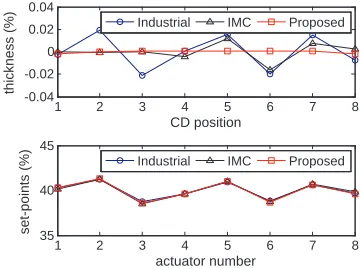
A number of simulations have been conducted to demon-strate how the controller performs, and three of these simu-lations are depicted in Figs. 4, 5, 6 and 7. These simusimu-lations have been conducted not only for the proposed controller but also for the industrial controller reported in [2] and [8] as well as another model-based controller reported in [3] to provide comparison. Figs. 4, 5 and 6 show the steady state CD thickness profile measured by the scanning gauge and the corresponding actuator set-points. Plots with squares are for the proposed controller and labelled “ Proposed” ; plots with circles are for the industrial controller and labelled “Industrial”; and plots with triangles are for the one reported in [3] and labelled “IMC” since it is also based on the IMC design. We assumed that the plastic film was divided into10

lanes [2]. To simulate what happens in real-life, the edges – the first and last lanes – were not controlled and left open-loop instead. Therefore, the figures do not show the first and last lanes. The y-axes represent thickness in percentage deviation from the mean, and the x-axes denote the CD position.

The reference model used for the industrial and IMC controllers is

˜

y(t) =h(z−1)kpGu(t) (37)

1 2 3 4 5 6 7 8

35 40 45

actuator number

set-points (%)

Industrial IMC Proposed

1 2 3 4 5 6 7 8

-0.04 -0.02 0 0.02 0.04

CD position

thickness (%)

Industrial IMC Proposed

Fig. 4. Simulation 1: Steady state CD thickness profile under normal operational conditions

which can be found in [8] and has been obtained using identification experiments similar to those reported in [1].

h(z−1) is given in (26), kp denotes a scalar gain, and G is the interaction matrix representing the steady state spatial response.

For the proposed controller design, the System Iden-tification ToolboxTM_{7 needs to be utilised to identify a}

reference model in the state-space form directly from the first-principles model, which simulates the plant. However, (37) has been identified directly from a real plant as opposed to the first-principles model. Although the first-principles model has been developed to simulate the plant, a mismatch between the plant and the first-principles model still exists. The proposed and existing controllers are all tested by ap-plication to the first-principles model and it therefore seems unfair for the existing controllers. To be fair, the reference model for the proposed controller has been identified from (37) instead of the first-principles model. If the reference model is identified from the first-principles model, improved performance of the proposed controller can be expected. It is also very important to point out that the industrial controller has been tuned to work optimally with the plant as opposed to the first-principles model, which in turn indicates that improved performance of the industrial controller can also be expected with improved tuning parameters.

Subsequently, all the controllers have been applied to the first-principles model and the simulation results are summarised as follows: In Simulation 1, the proposed con-troller achieves a significant improvement over the existing controllers under normal operating conditions as shown in Fig. 4. Although no disturbances are present, the set-points are not flat due to the mismatch between the reference model and the first-principles model. Although, the proposed controller design aims to minimise this mismatch, it can not be eliminated completely. Moreover, the reference model for every controller has been identified from (37) instead of the first-principles model leading to even larger model-plant mismatch.

1 2 3 4 5 6 7 8 35

40 45

actuator number

set-points (%)

1 2 3 4 5 6 7 8

-0.4 -0.2 0 0.2 0.4

CD position

thickness (%)

Industrial IMC Proposed Industrial IMC Proposed

Fig. 5. Simulation 2: Steady state CD thickness profile with fast-roll speed variation fromt= 0s; y-axis of upper plot has a different range from those in Fig. 4 and Fig. 6

1 2 3 4 5 6 7 8

35 40 45

actuator number

set-points (%)

Industrial IMC Proposed

1 2 3 4 5 6 7 8

-0.04 -0.02 0 0.02 0.04

CD position

thickness (%)

Industrial IMC Proposed

Fig. 6. Simulation 3: Steady state CD thickness profile with mass flow variation fromt= 3000s

±10%of the desired speed. The proposed controller achieves a significant improvement over the IMC controller and a slight improvement over the industrial controller.

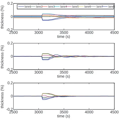
A polymer melt is fed into the die at a certain mass flow rate [2]. In Simulation 3, mass flow rate starts to vary suddenly from3000sin contrast to Simulation 2, where the variation occurs from 0s. The purpose of this simulation is to see how the controller responds to a disturbance appearing suddenly. Mass flow rate varies randomly within ±10% of the desired rate. Fig. 6 shows a significant improvement achieved by the proposed controller over the industrial con-troller but almost none over the IMC concon-troller. However, the dynamic response depicted in Fig. 7 indicates that the proposed controller rejects the distrubance significantly faster than the IMC controller.

Figs. 4, 5 and 6 depict that all the controllers have similar steady state actuator set-points. Despite the similar actuator set-points, the thickness profiles look quite different when they may be expected to be also similar. This is because while the set-points of the industrial controller reach the steady state with no fluctuation at all, the online optimisation, such as (36), used for the model-based controllers (i.e., proposed and IMC controllers) keeps updating the set-points,

2500 3000 3500 4000 4500

-0.2 0 0.2

time (s)

thickness (%)

2500 3000 3500 4000 4500

-0.2 0 0.2

time (s)

thickness (%)

2500 3000 3500 4000 4500

-0.2 0 0.2

time (s)

thickness (%)

lane1 lane2 lane3 lane4 lane5 lane6 lane7 lane8

Fig. 7. Simulation 3: Plots from top to bottom: Dynamic response of industrial controller, IMC controller and proposed controller

thereby keeping improving the thickness profiles even further with small but continuous changes to the set-points even at the steady state as shown in Fig. 7.

VII. CONCLUSION

This paper has reported on the development of a new model-based CD controller design and its application to a first-principles model. Simulation results, which provided comparison between the proposed controller and other exist-ing controllers under different disturbance scenarios, demon-strated improvements the proposed controller could possibly achieve over two other existing controllers.

REFERENCES

[1] A. Featherstone, J. VanAntwerp, and R. Braatz, Identification and control of sheet and film processes, ser. Advances in Industrial Control. London: Springer, 2000.

[2] S. Hur, J. Balderud, R. Katebi, and A. Taylor, “Cross directional control of a film manufacturing process using a first principle model,” in Proceedings of the European Control Conference 2009, Budapest, Hungary, 2009, pp. 4475–4480.

[3] W. P. Heath and A. G. Wills, “Design of cross-directional controllers with optimal steady state performance,” Centre for Integrated Dynamics And Control (CIDAC), University of Newcastle, NSW, 2380, Australia, Tech. Rep., 2002.

[4] A. Konak, D. W. Coit, and A. E. Smith, “Multi-objective optimization using genetic algorithms: A tutorial,” Reliability Engineering and System Safety, vol. 91, pp. 992–1007, 2006.

[5] J. Chen and R. J. Patton, Robust model-based fault diagnosis for dynamic systems, K.-Y. Cai, Ed. Kluwer Academic Publishers, 1999. [6] V. Zakian and U. Al-Naib, “Design of dynamical and control systems by the method of inequalities,”IEE Control Theory & Application, vol. 120(11), pp. 1421–1427, 1973.

[7] J. F. Frenzel, “Genetic algorithms,” IEEE Potentials, vol. 12(3), pp. 21–24, 1993.