Co-movements in Real Effective Exchange Rates : Evidence From the Dynamic Hierarchical Factor Model

D

EPARTMENT OF

E

CONOMICS

U

NIVERSITY OF

S

TRATHCLYDE

G

LASGOW

CO-MOVEMENTS IN REAL EFFECTIVE EXCHANGE RATES:

EVIDENCE FROM THE DYNAMIC HIERARCHICAL FACTOR

MODEL

B

Y

JUN NAGAYASU

N

O

13-18

S

TRATHCLYDE

Co-movements in Real Effective Exchange Rates: Evidence from

the Dynamic Hierarchical Factor Model

Jun Nagayasu∗

Abstract

We analyze and quantify co-movements in real effective exchange rates while considering the regional location of countries. More specifically, using the dynamic hierarchical factor model (Moench et al. (2011)), we decompose exchange rate movements into several latent components; worldwide and two regional factors as well as country-specific elements. Then, we provide evidence that the worldwide common factor is closely related to monetary policies in large advanced countries while regional common factors tend to be captured by those in the rest of the countries in a region. However, a substantial proportion of the variation in the real exchange rates is reported to be country-specific; even in Europe country-specific movements exceed worldwide and regional common factors.

JEL classification: F31

Keywords: Real effective exchange rates, dynamic hierarchical factor model, variance de-composition, Bayesian model averaging

∗

1

Introduction

In the past, some studies have been carried out on movements in exchange rates. The

co-movements, which can be measured by the sensitivity of one currency to another in regression

analysis or the simple correlation coefficient, are important since changes in one currency indeed

often affect the currency of other countries (e.g., McKinnon and Schnabl (2003)) particularly for

those implementing a flexible exchange rate regime. Furthermore, currency interdependence has

been examined in the context of inferring actual exchange rate regimes which may be deviating

from officially announced ones (e.g., Frankel and Wei (2008)).

The co-movements of exchange rates are also underlined during financial crisis periods;

de-terioration in one’s currency value almost simultaneously affecting others by, for example,

spec-ulative attacks (e.g., Gerlach and Smets (1995), Masson (1998)). Such an effect is often called

contagion in academic literature, and has been increasingly prominent over recent years when

a series of financial crises have affected the world economy. Recent examples include the 1997

Asian crisis which erupted in Thailand, the Lehman Shock (2008) in the US, and the European

sovereign debt crisis which started in Greece (2009). Each lead not only its own economy but

also its regional and/or the world economy into recession.

Generally, co-movements in financial asset prices and returns are shown to be time-varying

and increase during financial crises (see the next section), and as theoretical explanations, two

categories of propagation channels affecting other countries have been identified (see Forbes and

Rigobon (2001)). The first group is closely linked with economic fundamentals and tranquil

periods, and considers international trade, common economic policies, learning behaviors of

investors and global shocks as relevant propagation channels. The second group of channels is

more closely associated with crisis periods and is characterized by multiple equilibria in investors’

expectations, endogenous liquidity shocks and political influence over other countries.

However, previous studies have been carried out with rather different approaches and

fo-cuses. Such heterogeneity in research arises from different definitions of co-movements and

different approaches to measuring them.1 Indeed, there are many terminologies similar to

co-movements such as interdependence, cross country linkages, spillovers and contagion (see Forbes

and Rigobon (2001), Pesaran and Pick (2007)): while contagion is specific to financial crises and

the interdependence to tranquil periods, the rest are often used to refer to cross country

move-1

ments during any time period.2 Similarly, there are several approaches to analyze co-movements,

e.g., by looking at the correlation between exchange rates, the probability of speculative attacks

and the propagation of volatility.

In addition, given that a country normally has multiple trading partners, this effect should

be analyzed in a multi-country setting. However, a bilateral nominal exchange rate, often

vis-`

a-vis the US dollar, dominates the exchange rate literature (e.g., Macdonald and Taylor (1992)

and the next section), rather than a real effective exchange rate which is also important, e.g.,

as an indicator of the international competitiveness of a country.

Against this background, this paper analyzes and quantifies co-movements in real effective

exchange rates, mainly for advanced countries, while making use of information on the regional

location of countries. Unlike previous contagion studies which focused solely on spillovers during

crises, this paper will calculate and evaluate the size and evolution of spillovers, without making

a clear distinction between crisis and non-crisis periods.3 Therefore, here co-movements are

synonymous with cross country linkages and spillovers, and in this context, we attempt to

estimate worldwide and regional common factors by using an advanced statistical method and

identify countries which are influential over other exchange rates.

Thus the distinguishing features of this paper are: 1) decomposition of the real effective

ex-change rates of 30 countries into several factors (hierarchies) by applying the recently developed

statistical method, the dynamic hierarchical factor model (Moench et al. (2011)), 2)

quantifi-cation of the contribution of each hierarchy to the total variation in exchange rates, and 3)

identification of countries who are influential over other countries’ exchange rates. However,

un-like contagion studies, this paper does not emphasize the direction of causality from one country

to another.

The paper consists of 5 sections. In the next section, we summarize previous studies focusing

on statistical methods which can be used to estimate co-movements in exchange rates. Section 3

describes the dynamic hierarchical factor model which have recently been proposed by Moench

et al. (2011)). Section 4 describes the data and presents our estimates of co-movements in

exchange rates from the dynamic hierarchical factor model; furthermore, this section investigates

the driving forces of co-movements by means of the Bayesian Model Averaging (BMA) method.

2

For example, Pesaran and Pick (2007) make a clear distinction between contagion and interdependence; the latter referring to spillover effects during the tranquil period.

3

This paper ends with our conclusion in Section 5.

2

Review of Measuring the Co-movements

Co-movements in financial asset prices have frequently been studied in the context of the

eval-uation of financial crises and the international capital market integration, and equity returns

rather than exchange rates have been the main focus in previous studies. Therefore, these

stud-ies have profound implications for building a financial portfolio, e.g., see the capital asset pricing

model. However, the same concept of co-movements and statistical approach can be applied to

exchange rate analysis; therefore, we shall review previous literature by focusing on the

sta-tistical methodologies used to measure them for a variety of financial assets. Such academic

literature seems to have employed one of the following approaches.

The traditional and probably most popular approach is to use correlation measures between

international stock returns, and increased correlation is regarded as evidence of increased

cross-country linkages. This can be carried out either by simply calculating correlation coefficients

among stock returns or estimating the stock return equation of one country with other countries’

stock returns as explanatory variables. Classic studies include Makridakis and Wheelwright

(1974) that showed unstable interrelationships in the major stock exchanges of the world. King

and Wadhwani (1990) reported increased correlation at the time of the October 1987 crush. A

similar result has been reported for more recent crises by a number of researchers (Longin and

Solnik (1995), Liu et al. (1998), Reinhart and Calvo (1996), Bayoumi et al. (2007)). However,

there are potential problems. Obviously, the regression based approach requires an exogeneity

assumption about explanatory variables. But it may be difficult to justify this assumption using

volatile financial asset data. Furthermore, Forbes and Rigobon (2002) argue that the regression

analysis should take into account market volatility which differs during crisis and non-crisis

periods, and they conclude that once this effect is considered, no evidence of contagion is found

in Black Monday (1987), the Mexican currency crisis (1994) or the Asian crisis (1997).

Second, co-movements can be estimated using the factor model or the principal components

approach. The factor model is often used to distinguish between worldwide and country-specific

elements, and according to this approach, increases in the proportion of the worldwide factor

become evidence of higher cross-country linkages (Koedijk and Schotman (1989), Dungey (1999),

approach. For example, Nellis (1982) analyzed financial market integration using corporate and

government bonds with the expectation that their yields will be dominated by common factors

in a highly integrated financial market. Similarly, Volosovych (2013) studied financial market

integration utilizing government bond yields from 1875 to 2009 and provided evidence of a higher

integration from the data through the end of the 20th century. These traditional approaches

often hinge upon the assumption of the stationarity of data. In this regard, Eickmeier (2009)

and Byrne and Nagayasu (2012) used a nonstationary dynamic factor model (Bai and Ng (2004))

to highlight homogeneity in European financial markets.

However, the number of countries under investigation from these methods seems to be rather

limited, and there is a strong tendency for research to focus on advanced countries. Using the

factor model, Koedijk and Schotman (1989) studied the exchange rates of 15 industrialized

countries, Dungey (1999) analyzed 6 Pacific Rim currencies and Cayen et al. (2010) dealt with 6

countries against the US dollar. Using the principal components method, Nellis (1982) employed

the bond yields of 5 advanced countries, and Volosovych (2012) studied the government bond

yields of 15 industrialized countries. Using a nonstationary factor model, Eickmeier (2009)

considered 7 core Euro area countries and Byrne and Nagayasu (2012) focused on 11 emerging

European countries.

The limited coverage of countries seems to be due to several reasons. Obviously, data

avail-ability is one issue for deciding the number of countries under investigation, at least in the

past. However, more countries now exist in the world; especially, the number of countries has

increased after the breakdown of socialist countries, and today there are a number of countries

who have disseminated a reasonably long history of data. Second, the economic interpretation

of commonality may become more difficult with a large data set because the number of common

factors often increases along with an expansion in country coverage. This also may have become

a reason for the analysis of small data sets.

However, over the last decade much progress has been made in estimating multiple

com-monality in large data sets, especially in the area of studies on business cycles and general

commodity (not financial asset) inflation. Using a modified factor model, Forni et al. (2000),

Kose et al. (2003) and Foerster et al. (2011) analyzed international or domestic business cycles

for a large number of countries or economic sectors. The recent relevant studies on inflation

Due to the increased complexity of the model, it has become standard to estimate the model

using the Bayesian estimation technique.

This study follows the second strand of the literature (i.e., the factor model) by extending it

in a number of ways. In particular, rather than a two level classification, we consider four level

hierarchies in our estimation. This is an essential modification in order to study many countries

with a number of economically interpretable common factors. The increased complexity of the

model cannot be estimated by conventional statistical methods and thus will be executed by the

Bayesian method.

3

Econometric Method: The Factor Model

Correlation between economic variables has been of interest to economists since economic events

are often highly correlated with one another. As reviewed in previous studies, classic studies

used the factor model to extract commonality among a panel of stationary variables. One

recent extension is to decompose data into common and idiosyncratic factors (i.e., a two level

decomposition) in a nonstationary environment (Bai and Ng (2004)). Another extension is

Moench et al. (2011) that has proposed the four level hierarchical factor model for a panel of

stationary variables. The latter is also attractive in the presence of multiple common factors.

By imposing extra information when grouping countries into hierarchies, this model facilitates

researchers in identifying and interpreting each factor. Furthermore, they argue that this extra

information results in reduction in computational burdens compared with Kose et al. (2003)

who also proposed the Bayesian method to decompose a large data set. Here we make use of

geographical information since adjacent countries tend to possess similar cultures and economic

structures, to be very important trade partners, and to share common trading hours through

which investors receive information simultaneously (see e.g., Goldstein (1998))

Following closely the notation used in Moench et al. (2011), this four level decomposition of

a vector Zbsnt can be written, from low to high level, as:

Zbsnt = ΛHbsnHbst+eZbsnt (1)

Hbst = ΛGbsGbt+eHbst (2)

where the Greek letters are loadings, and t is time (t = 1, . . . , T), and components which cannot be explained by the factors (F,Gand H) are treated as residuals (e). Thus, we assume that the universal factors affect more regional factors; the worldwide factor (F) affects regional factors (G), andGinfluences H which is more region specific.

In Eqs 1 to 3, the lowest (i.e., individual) level classification is characterized as Zbsnt

con-taining individually the exchange rates of all countries (Eq. 1). Each exchange rate movement is

decomposed to a regional level common factorHbst and country-specific elements eZbsnt. Since

the latter do not have a common factor, country-specific elements are assumed to be independent

across countries.

In our analysis, there are two levels of regional classification (Levels 2 and 3, Table 1). Level

2 consists of 4 regional factors; namelyH11t for the Euro area,H12t for the non-Euro European

area,H21tfor the Asia-Pacific area, andH22tfor the American area, (i.e., b= 1,2 ands= 1,2).

This classification is based largely on geographical information. But a distinction is made

between Euro zone members and non-members, since within the single currency area nominal

exchange rates are identical among member countries, and thus a high level of correlation is

expected among them.4

Another regional classification (Level 3) is based on whether or not countries are in Europe;

European factors are shown as G1t, and non-Europeans as G2t (b= 1,2). These factors affect

the second level regional factors. In turn, former regional factors (G1t and G2t) are influenced

by a worldwide commonality (F) (Eq. 3). Here, one common factor is assumed to exist in each group (i.e., G1, G2, H11, H12, H21, H22 andF) in our model.5

For the estimation, each factor is assumed to be stationary and is in the form of the first-order

autoregression.

Ft = ρFFt−1+εF t, εF t ∼N(0, σ2F)

eGbt = ρGbeGbt−1+εGbt, εGbt∼N(0, σ2Gb)

eHbst = ρHbseHbst−1+εHbst, εHbst∼N(0, σ2Hbs)

eZbsnt = ρZbsneZbsnt−1+εZbsnt, εZnbst ∼N(0, σZbsn2 )

4_{Our classification method may be ad hoc but is largely consistent with Koedijk and Schotman (1989).} 5

The abovementioned model is estimated using the Markov Chain Monte Carlo (MCMC)

method. We follow the assumption about the prior distribution used in Moench et al. (2011); for

example, the prior distribution of parameters are assumed to be standard normal, Λ, ρ∼N(0,1), and that of variance an inverse of the scaledχ2 distribution.6 The initial values for latent vari-ables are estimated by the principle components approach. In order to obtain reliable estimates,

the first 50,000 out of our 100,000 draws are discarded, and every 50th observation from the

remaining 50,000 draws is used for the analysis. This leaves us 1,000 draws for each parameter

at each point in time. Furthermore, convergence diagnostics are calculated based on the Geweke

test, but are not reported here for the sake of brevity.

4

Empirical results

4.1 Estimation of Common Factors

Real effective exchange rate data are obtained from the International Financial Statistics (IFS) of

the International Monetary Fund. They (IFS code..REUZF, 2005=100) are constructed using

the consumer price index and weights determined by the size of trade (unit values) to each

trading partner, and cover the sample period from 1980Q1 to 2012Q2 for 30 countries, most

of which are advanced ones (see Table 1).7 These countries are classified as Group 1 (12 Euro

countries), Group 2 (10 non-Euro European countries), Group 3 (4 Asia-Pacific countries) and

Group 4 (4 American countries). In the subsequent analysis, we analyze exchange rate growth,

i.e., the first difference of log exchange rates (Log(St/St−1)×100), in order to be congruent with

a priori assumption of the data required for the factor model.

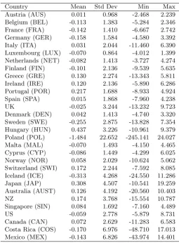
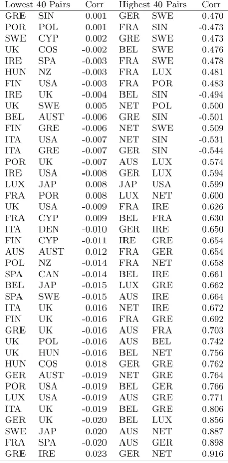
The basic statistics are summarized in Table 2, and the conventional correlations (the

highest-and lowest-40) of exchange rate pairs are listed in Table 3. The sign of the average exchange

rate suggests that the direction of exchange rate movements is quite diversified; half of the

countries have experienced an exchange rate increase (Table 2). Furthermore, among them, the

6_{Our estimation is based on the Matlab codes of Professor Ng which are disseminated on her homepage. Details}

of assumptions about the prior distributions are stated there. The scale factor for the scaled inverseχ2 is set as 0.01.

7

Polish Zloty rate has experienced high volatility. The volatility can be measured by the standard

deviation and is closely associated with acceleration in domestic inflation from the late 1980s to

the early 1990s. Otherwise, other exchange rates appear quite comparable.

In addition, as expected, high correlation is obtained from a pair of Euro member countries,

particularly Germany and the Netherlands (Table 3). In contrast, the lowest correlation is

obtained between Greece and Singapore, countries from different geographical groups. As in

the classic principle component approach, all the data are standardized to have zero mean and

variance equal to one before we implement the dynamic hierarchical factor model.

Figures 1 to 3 plot estimates of the common factors from the dynamic hierarchical factor

models, where all 1,000 observations are shown for each time period. They suggest that these

factors are stationary regardless of the level of hierarchies, and the non-European common factor

(G2) which includes the US, exhibits sharper changes around 2008/09 than the European factor

(G1) in response to adverse effects from the Lehman Shock. Furthermore, the European factor

(G1) is more tightly distributed than the non-European factor, suggesting less uncertainty about

the estimates for Europe and homogeneity of their exchange rates. Apart from these points, it

is very difficult to draw any concrete conclusions from these graphs.

Therefore, in order to understand better these common factors, we carry out the variance

decomposition analysis using the common factors which are equal to the average values in Figures

1 to 3 at each point in time. The total variance of exchange ratesV ar(Zbsn) can be decomposed

to:

V ar(Zbsn) =γF(V ar(F)) +γG(V ar(eGb)) +γH(V ar(eHbs)) +γG(V ar(eZbsn)) (4)

whereγ is a composite of parameters, Λ in Eq. (1) to (3), and the following ratios are presented in Table 4

γF(V ar(F))/V ar(Zbsn)

γG(V ar(eGb))/V ar(Zbsn)

γH(V ar(eHbs))/V ar(Zbsn)

γG(V ar(eZbsn))/V ar(Zbsn)

(5)

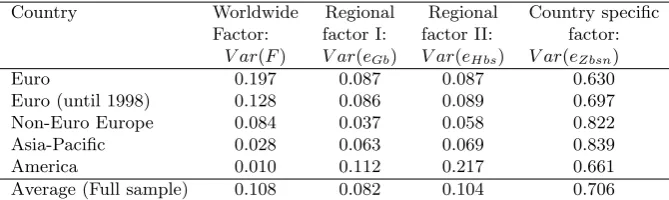
From this table, we can report several findings. First, there is a clear difference between

country-specific element is generally most significant (71% on average, Table 4). This element

is more important for a group which contains countries with a heterogeneous background. In

this regard, the country-specific variation is least important among the Euro members (Group

1) but still accounts for nearly 60% of the total variation.

There may be two reasons for this outcome. One obvious reason is that our observations

include the pre-Euro period. Prior to 1999, there is heterogeneity in nominal exchange rates of

euro candidate countries although they had been making efforts to meet the convergence criteria.

Second, given that their nominal rates are identical after the introduction of the Euro,

hetero-geneity in prices and trading partners seem to be significantly different among Euro member

countries. This implies the presence of a diversified external competitiveness within the Euro

area.

With respect to other regions, the non-Euro European and Asia-Pacific groups have exhibited

a similar proportion of country-specific effects (over 80%). This outcome for non-Euro European

countries may be due to their heterogeneities among countries; this group consists of member

and non-member states of the European Union (EU) as well as countries which have recently

joined the Euro zone (Table 1).

Table 4 also shows that country-specific effects are relatively low in American countries

(Group 4) although they are slightly higher than the level of Group 1. These results likely

reflect the fact that 3 countries (the USA, Canada and Mexico) in this group form NAFTA,

leading their markets to become more homogeneous.

Finally, given the fact that the Euro was introduced in January 1999, we have repeated

the same analysis this time for the Euro Group. The results are also reported in Table 4 and

suggests a slight increase (drop) in the importance of country-specific (worldwide) components

from the data prior to 1999. It implies that, while the relationship with regional factors remains

relatively similar to the pre-Euro period, real exchange rates in the Euro members have been

more synchronized with and have become more dominant over the worldwide factor after 1999.

4.2 Countries Influential over the Common Factors

Then what are the driving forces of these common factors? Economic theory suggests that

real exchange rate would be determined by the real interest rate differential or the productivity

Here we use real interest rates which seem to be available for more countries, and shall summarize

below their theoretical link following Obstfeld and Kenneth (1996). Their derivation of the model

is more attractive than the conventional one using only the purchasing power theorem and the

covered interest rate parity condition (see MacDonald and Nagayasu (2000)) in the sense that

sticky prices are considered in the model.

Let’s consider domestic inflation which can be explain by the Dornbusch type inflation

spec-ification for an open economy.

∆pt+1 =γ(ydt −y¯t) + ∆st+1+ ∆˜p∗t+1 (6)

where yd_t is the demand for home country output, sis the nominal exchange rate and p is the price. Because all variables are in log form, and ∆ represents the differenced variable; therefore,

∆pt+1 = pt+1 −pt becomes inflation. A variable with a bar indicates a natural level, and a

foreign variable is denoted with an asterisk. In the presence of multiple partner countries, the

latter can be thought of as a weighted average of foreign variables; thus the tilde suggests the

weighted average of prices in partner countries. Theγ >0 implies that home inflation increases due to excessive demand for home products, exchange rate depreciation, and increases in foreign

inflation. Otherwise, there is no market clearance, i.e., ∆pt+1 6= 0.

Further, the demand for home products (y_td) is assumed to be expressed as:

y_td= ¯yt+δ(st−pt+ ˜p∗t−q¯) (7)

where δ >0. For simplicity, the long-run (or equilibrium) real exchange rate is assumed to be fixed here. According to this equation, the demand for domestic goods exceeds its natural level

to an extent proportional to the level of currency misalignment.

Using the definition of the real exchange rate (qt≡st−pt+ ˜p∗t) and the uncovered interest

parity condition (∆st+1 =it−˜i∗t, whereiis the nominal interest rate), Eqs. 6 and 7 yield:

∆pt+1 =γδ(qt−q¯) +it−˜i∗t + ∆˜p∗t+1 (8)

the real exchange rate, we can obtain the following relationship:

qt= ¯q−

1

γδ(rt−˜r

∗

t) (9)

Since all parameters are theoretically positive, this equation asserts that there would be home

currency depreciation when the real interest rate falls at home. Given that many advanced

countries have recently been experiencing a minimal inflation level, the nominal interest rate

guided by monetary policy has a close link with the exchange rate.

Indeed there are many previous studies investigating the relationship between real exchange

rates and real interest rates. Early studies tend to cast doubt on the credibility of this

rela-tionship (Edison and Pauls (1993), Edison and Melick (1999)); however, stronger evidence is

reported by more recent studies (MacDonald and Nagayasu (2000), Byrne and Nagayasu (2010))

when taking into account the possibility of nonstationary elements in exchange rates and

inter-est rates in the panel data context. Since the latter studies utilize cross country information

and thus yield more reliable statistical results, we could base our analysis on this theoretical

framework.

For the estimation, we consider the equation of exchange rate changes which is consistent

with our derivation of common factors. Furthermore, since there are several components in real

effective exchange rates, we shall estimate each factor using real interest rate data, based on the

following liner equation.

∆qCom_t =c+β1∆rt+β2∆˜rt∗+ut (10)

whereq_tCom is the common factor in the real effective exchange rates, and can be the worldwide factor (Com =F) or regional common factors (Com =G1, G2, H11, H12, H21 or H22). The ut

is a residual, and the theoretical sign for this equation is β1 <0 and β2 >0 as suggested by

Eq. 9. For the estimation, the real interest rate of each country is directly introduced in the

specification rather than assigning a weight to foreign variables prior to the estimation as in Eq.

10 .

∆q_tCom=c+β1∆r1t+β2∆r2∗t+β3∆r3∗t+...+βj∆rjt∗ +ut (11)

relation-ship in order to clarify the relevance of countries to the common factors. The distinguishing

feature of the BMA is to extend the standard Bayesian statistical method which addresses

parameter uncertainty to also considering model uncertainty. This approach has drawn

con-siderable interests from researchers over recent decades, and has been applied to identifying

relevant variables for explaining economic growth, which potentially has a number of candidate

explanatory variables (Fernandez et al. (2001)).

The concept of the BMA can be summarized very concisely using the following equation.

(See Appendix about more detailed explanations about the BMA.) For a normal linear equation

withk real interest rates, a parameter from the BMA can be summarized as:

βBM A= k

X

j=1

wjβj (12)

where wj is a weight attached to parameters βj for model specification, j; each model has a

different combination of explanatory variables. Parametersβj are estimated by the conventional

Bayesian method and thus parameter uncertainty will be addressed here. Consideration of

weight, wj, captures model uncertainty. With the intercept term always in the specification,

the BMA evaluates the importance of 2k models which will be estimated by the Markov Chain

Monte Carlo model composition (M C3)(Madigan et al. (1995)).

Here, most data are based on money market nominal rates (IFS code: 60B..ZF) but in their

absence, deposit rates (60L..ZF) are used as alternatives.8 We obtain real interest rates by

subtracting inflation rates from the nominal interest rates, and calculate inflation rates using

the consumer price index (CPI) (IFS code: 64...ZF). Since the CPI is not available from the IFS

for Germany or the UK, their inflation rates are obtained from the OECD Main Indicators and

the Office of National Statistics, UK, respectively. Due to data availability, our data set does

not cover the real interest rates of all but 16 countries.9 This leaves us analysis of 216(= 65,536) models.

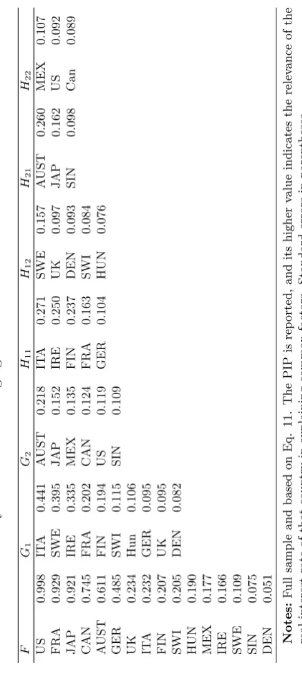
Table 5 reports BMA results for each common factor. Model uncertainty is shown as the

posterior inclusion probability (PIP) which is the sum of posterior model probabilities (PMP)

from all models (see Appendix). The PIP shows the likelihood of appearance in the common

8

Deposit rates are used for France, Hungary and Mexico.

9

factor equations, and its high value can be considered as more relevant to explaining common

factors. Against this background, advanced countries; notably, the US, France and Japan, are

reported to be most relevant to the worldwide common factor. Their PIP exceeds more than

90 percent, which confirms that large economies become more influential over the worldwide

variation in exchange rates. Because there is a substantial difference in the PIP among countries,

our result is also consistent with the asymmetric effects of monetary policy which have been

identified in the past. For example, Bansal and Dahlquist (2000) and Byrne and Nagayasu

(2012) discuss that US monetary policy is very influential over emerging markets and the US

influence remains higher than domestic ones even for other advanced economies (Nagayasu

(2003)).

As we move on to regional factors, some other countries which are not regarded as most

relevant to the worldwide common factor, are found to be closely related to regional factors.

For example, the interest rates of Italy and Sweden are reported to be closely associated with

G1, and Australia with G2. Similarly, Italy and Ireland exhibit a close association with H11

while France and Germany are less relevant to this level of the common factor. InH22, Mexico

is found to be more relevant than the US and Canada which are reported to be closely linked

with the worldwide factor. Obviously, this is a general observation, but is consistent with the

conventional belief.

Furthermore, the different magnitude of our estimates (PIP) in different common factors

implies that the worldwide common factor is more closely associated with interest rates compared

with regional factors; its PIP is much higher than that found from regional factors. Thus this

finding implies that the determinants of regional factors are more complex and this underlines

the potential importance of other economic and financial factors. The increase in this complexity

can be understood by Eqs 1 to 3 where lower level hierarchical factors are driven by more region

specific and heterogeneous information.

Needless to say, Table 5 does not give much information about country specific factors, but

as discussed, our study (Table 4) shows that more than half of variation in real effective exchange

rates are attributable to country specific factors. The results remain valid even for the Euro

5

Conclusion

Given that exchange rates are believed to be highly correlated among countries, we calculate

co-movements in real effective exchange rates using the recently developed data decomposition

method (Moench et al. (2011)). Then, our results suggest that the evolution of real effective

exchange rate changes is rather country-specific. As expected, the country-specific elements

are less significant within the Euro area compared with other regions, and their importance

has dropped after the introduction of the Euro. However, these components still account for

around 60% of the total variation, implying heterogeneous inflation and external competitiveness

among member countries. This is in sharp contrast to the expectation that real exchange rate

movements are dominated by common factors in a single currency union, and underlines the

importance of both idiosyncratic and 3rd country effects when understanding exchange rate

dynamics. Therefore, a single country analysis remains important and should deliver valuable

information even when assessing the economic conditions of a single currency area.

Our further analysis has identified countries which are influential over common movements in

real effective exchange rates using the BMA. In this paper, the empirical analysis is carried out

within the theoretical framework of real exchange rates and interest rates, and thus our study

is closely related to the influence of monetary policy over exchange rates. Then we report that

the worldwide common factor is often associated with interest rates in large advanced countries,

notably the USA. Therefore, US monetary policy is confirmed to be very influential over world

exchange rates. By contrast, regional factors are to a larger extent affected by economic and

Appendix. Bayenesian Model Averaging

This appendix summarizes the concept and specific assumptions used for the Bayesian Model Averaging (BMA) in this paper. (See also Koop (2003) regarding the general concept of the BMA.) Maintaining the mathematical notation used in the main text, the BMA is summarized below.

With kexplanatory variables, the posterior for the parameters for Mj can be written using

the Bayesian rule as:

p(βj|y, X) =

2k

X

j=1

p(β|Mj, y, X)p(Mj|y, X) (13)

It states that the posterior for the parameters of interest consists of the weighted average of the posterior distribution of the parameters from all models and the posterior model probabilities (PMP). Furthermore, the PMP can be expressed as:

p(Mj|y, X) =

p(y|Mj, X)p(Mj)

p(y|X) (14) Since the denominator is constant over the models, we could focus only on the numerator;p(Mj)

is assumed to follow a uniform prior probability for each model,p(Mj)∝1, andp(Mj) = 1/2k.

Then dropping this term which is constant over models, the PMP can be expressed as:

p(Mj|y, X) =

p(y|Mj, X)

P2k

i=1p(y|Mi, X)

(15)

The posterior inclusion probably (PIP) is the sum of PMP from all models including variable

xh:

p(xh|y, X) =

X

i:xh∈Mj

p(Mi|y, X) (16)

For more specific assumptions, we follow Zellner’sgprior. In other word, based on a Bayesian linear model, we consider

βj|g∼N(0, σ2g(Xj0Xj)−1) (17)

where g measures the level of uncertainty and is set as g =max(T, K2); uncertainty increases along with rises in g. Then the marginal likelihood for Mj is:

p(y|Mj, X)∝

g g+ 1

kj

2 ₁

g+ 1y

0

Pxjy+

g

g+ 1(y−y)

0

(y−y)

−T−1

2

(18)

where PXj =IT −Xj(X

0 jXj)

−1_X0 j.

References

Bai, J. and S. Ng (2004). A panic attack on unit roots and cointegration. Econometrica 72(4), 1127–1177.

Bai, J. and S. Ng (2007). Determining the number of primitive shocks in factor models. Journal of Business & Economic Statistics 25, 52–60.

Bansal, R. and M. Dahlquist (2000). The forward premium puzzle: different tales from developed and emerging economies. Journal of International Economics 51(1), 115–144.

Bayoumi, T., G. Fazio, M. Kumar, and R. MacDonald (2007). Fatal attraction: Using distance to measure contagion in good times as well as bad. Review of Financial Economics 16(3), 259 – 273.

Bernanke, B., J. Boivin, and P. S. Eliasz (2005). Measuring the effects of monetary policy: A factor-augmented vector autoregressive (favar) approach. The Quarterly Journal of Eco-nomics 120(1), 387–422.

Byrne, J. P. and J. Nagayasu (2010). Structural breaks in the real exchange rate and real interest rate relationship. Global Finance Journal 21(2), 138–151.

Byrne, J. P. and J. Nagayasu (2012). Common factors of the exchange risk premium in emerging european markets. Bulletin of Economic Research 64, s71–s85.

Canova, F. and M. Ciccarelli (2009). Estimating multicountry var models*. International Economic Review 50(3), 929–959.

Cayen, J.-P., D. Coletti, R. Lalonde, and P. Maier (2010). What drives exchange rates? new evidence from a panel of u.s. dollar bilateral exchange rates. Technical report, Bank of Canada Working Paper 2010-5.

Dungey, M. (1999). Decomposing exchange rate volatility around the pacific rim. Journal of Asian Economics 10(4), 525 – 535.

Edison, H. J. and W. R. Melick (1999). Alternative approaches to real exchange rates and real interest rates: Three up and three down. International Journal of Finance & Economics 4(2), 93–111.

Edison, H. J. and B. D. Pauls (1993). A re-assessment of the relationship between real exchange rates and real interest rates: 1974-1990. Journal of Monetary Economics 31(2), 165–187.

Eickmeier, S. (2009). Comovements and heterogeneity in the euro area analyzed in a non-stationary dynamic factor model. Journal of Applied Econometrics 24(6), 933–959.

Fernandez, C., E. Ley, and M. F. J. Steel (2001). Model uncertainty in cross-country growth regressions. Journal of Applied Econometrics 16(5), 563–576.

Foerster, A. T., P.-D. G. Sarte, and M. W. Watson (2011). Sectoral versus aggregate shocks: A structural factor analysis of industrial production. Journal of Political Economy 119(1), 1 – 38.

Forbes, K. J. and R. Rigobon (2002). No contagion, only interdependence: Measuring stock market comovements. Journal of Finance 57(5), 2223–2261.

Forni, M., M. Hallin, M. Lippi, and L. Reichlin (2000). The generalized dynamic-factor model: Identification and estimation. The Review of Economics and Statistics 82(4), pp. 540–554.

Frankel, J. and S.-J. Wei (2008). Estimation of de facto exchange rate regimes: Synthesis of the techniques for inferring flexibility and basket weights. IMF Staff Papers 55(3), 384–416.

Gerlach, S. and F. Smets (1995). Contagious speculative attacks. European Journal of Political Economy 11(1), 45–63.

Goldstein, M. (1998). Asian Financial Crisis: Causes, Cures and Systemic Implications, The. Number pa55 in Peterson Institute Press: All Books. Peterson Institute for International Economics.

King, M. A. and S. Wadhwani (1990). Transmission of volatility between stock markets. Review of Financial Studies 3(1), 5–33.

Koedijk, K. and P. Schotman (1989). Dominant real exchange rate movements. Journal of International Money and Finance 8(4), 517 – 531.

Koop, G. (2003). Bayesian Econometrics. John Wiley & Sons.

Kose, M. A., C. Otrok, and C. H. Whiteman (2003). International business cycles: World, region, and country-specific factors. American Economic Review 93(4), 1216–1239.

Liu, Y., M.-S. Pan, and J. Shieh (1998). International transmission of stock price move-ments: Evidence from the u.s. and five asian-pacific markets. Journal of Economics and Finance 22(1), 59–69.

Longin, F. and B. Solnik (1995). Is the correlation in international equity returns constant: 1960-1990? Journal of International Money and Finance 14(1), 3–26.

MacDonald, R. and J. Nagayasu (2000). The long-run relationship between real exchange rates and real interest rate differentials: A panel study. IMF Staff Papers 47(1), 5.

Macdonald, R. and M. P. Taylor (1992). Exchange rate economics: A survey. Staff Papers -International Monetary Fund 39(1), pp. 1–57.

Madigan, D., J. York, and D. Allard (1995). Bayesian graphical models for discrete data.

International Statistical Review / Revue Internationale de Statistique 63(2), pp. 215–232.

Makridakis, S. G. and S. C. Wheelwright (1974). An analysis of the interrelationships among the major world stock exchanges. Journal of Business Finance & Accounting 1(2), 195–215.

Masson, P. R. (1998). Contagion-monsoonal effects, spillovers, and jumps between multiple equilibria. IMF Working Papers 98/142, International Monetary Fund.

McKinnon, R. and G. Schnabl (2003). Synchronised business cycles in east asia and fluctuations in the yen/dollar exchange rate. The World Economy 26(8), 1067–1088.

Moench, E., S. Ng, and S. Potter (2011). Dynamic hierarchical factor models. Review of Economics and Statistics, forthcoming.

Nagayasu, J. (2003). Asymmetric effects of monetary indicators on the japanese yen. Japan and the World Economy 15(2), 143–159.

Nellis, J. G. (1982). A principal components analysis of international financial integration under fixed and floating exchange rate regimes. Applied Economics 14(4), 339–354.

Obstfeld, M. and R. S. Kenneth (1996). Foundations of International Macroeconomics. MIT Press.

Pesaran, M. H. and A. Pick (2007). Econometric issues in the analysis of contagion. Journal of Economic Dynamics and Control 31(4), 1245 – 1277.

Reinhart, C. M. and S. Calvo (1996). Capital flows to latin america: Is there evidence of contagion effects? In G. A. Calvo, M. Goldstein, and E. Hochreiter (Eds.), Private Capital Flows to Emerging Markets After the Mexican Crisis, Peterson Institute Press: Chapters, pp. 151–171. Peterson Institute for International Economics.

Table 1: List of Countries and Hierarchical Classification

Level 4 All countries (F)

Level 3 Europe (G1) Non-Europe (G2)

Level 2 Group 1 (H11) Group 2 (H12) Group 3 (H21) Group 4 (H22)

Euro Non-Euro Europe Asia-Pacific America Level 1 [Z] Austria UK Japan US

Belgium Denmark Australia Canada France Sweden NZ Costa Rica Germany Hungary Singapore Mexico Italy Poland

Luxembourg Malta Netherlands Cyprus Finland Norway Greece Switzerland Ireland Iceland Portugal

Spain

Notes:Malta and Cyprus are Euro member countries, but are treated here as

Non-Euro Non-European countries since their entry date is very recent (2008). Common factors are denoted asF,G, andH, andZ are country vectors.

Table 2: Basic Statistics for Changes in Exchange Rates

Country Mean Std Dev Min Max Austria (AUS) 0.011 0.968 -2.468 2.239 Belgium (BEL) -0.113 1.383 -5.284 2.346 France (FRA) -0.142 1.410 -6.667 2.742 Germany (GER) -0.158 1.584 -4.580 3.392 Italy (ITA) 0.031 2.044 -11.460 6.390 Luxembourg (LUX) -0.070 0.864 -4.012 1.399 Netherlands (NET) -0.082 1.413 -3.727 4.274 Finland (FIN) -0.101 2.136 -9.539 5.635 Greece (GRE) 0.130 2.274 -13.343 5.811 Ireland (IRE) 0.120 2.136 -5.890 6.286 Portugal (POR) 0.217 1.688 -8.933 4.924 Spain (SPA) 0.015 1.868 -7.960 4.238 UK -0.025 3.244 -13.232 9.723 Denmark (DEN) 0.042 1.413 -4.740 3.320 Sweden (SWE) -0.255 2.875 -13.828 7.354 Hungary (HUN) 0.437 3.226 -10.961 9.379 Poland (POL) -1.484 22.652 -245.141 24.027 Malta (MAL) -0.070 1.493 -4.150 4.465 Cyprus (CYP) -0.086 1.449 -4.299 6.025 Norway (NOR) 0.058 2.029 -10.624 5.062 Switzerland (SWI) 0.172 2.244 -7.592 8.085 Iceland (ICE) -0.313 4.268 -24.550 11.286 Japan (JAP) 0.308 4.507 -10.541 19.259 Australia (AUST) 0.126 4.192 -20.560 10.403 NZ 0.174 3.768 -15.554 10.787 Singapore (SIN) 0.084 1.692 -7.160 4.489 US -0.059 2.778 -5.879 8.731 Canada (CAN) 0.072 2.629 -11.283 6.583 Costa Rica (COS) -0.170 6.976 -48.710 17.013 Mexico (MEX) -0.143 6.826 -43.974 14.401

Table 3: Correlations Between Exchange Rate Changes

Lowest 40 Pairs Corr Highest 40 Pairs Corr GRE SIN 0.001 GER SWE 0.470 POR POL 0.001 FRA SIN -0.473 SWE CYP 0.002 GRE SWE 0.473 UK COS -0.002 BEL SWE 0.476 IRE SPA -0.003 FRA SWE 0.478 HUN NZ -0.003 FRA LUX 0.481 FIN USA -0.003 FRA POR 0.483 IRE UK -0.004 BEL SIN -0.494 UK SWE 0.005 NET POL 0.500 BEL AUST -0.006 GRE SIN -0.501 FIN GRE -0.006 NET SWE 0.509 ITA USA -0.007 NET SIN -0.531 ITA GRE -0.007 GER SIN -0.544 POR UK -0.007 AUS LUX 0.574 IRE USA -0.008 GER LUX 0.594 LUX JAP 0.008 JAP USA 0.599 FRA POR 0.008 LUX NET 0.600 UK USA -0.009 FRA IRE 0.626 FRA CYP 0.009 BEL FRA 0.630 ITA DEN -0.010 GER IRE 0.650 FIN CYP -0.011 IRE GRE 0.654 AUS AUST 0.012 FRA GER 0.654 POL NZ -0.014 FRA NET 0.658 SPA CAN -0.014 BEL IRE 0.661 BEL JAP -0.015 LUX GRE 0.662 SPA SWE -0.015 AUS IRE 0.664 ITA UK 0.016 NET IRE 0.672 FIN UK -0.016 FRA GRE 0.692 GRE UK -0.016 AUS FRA 0.703 UK POL -0.016 AUS BEL 0.742 UK HUN -0.016 BEL NET 0.756 HUN COS 0.018 GER GRE 0.762 GER AUST -0.019 NET GRE 0.764 POR USA -0.019 BEL GER 0.766 LUX USA -0.019 AUS GRE 0.771 ITA UK -0.019 BEL GRE 0.806 GER UK -0.020 BEL LUX 0.856 SWE JAP 0.020 AUS NET 0.887 FRA SPA -0.020 AUS GER 0.898 GRE IRE 0.023 GER NET 0.916

Notes: See Table 2 for abbreviation of country

Table 4: Variance Decomposition

Country Worldwide Regional Regional Country specific Factor: factor I: factor II: factor:

V ar(F) V ar(eGb) V ar(eHbs) V ar(eZbsn)

Euro 0.197 0.087 0.087 0.630 Euro (until 1998) 0.128 0.086 0.089 0.697 Non-Euro Europe 0.084 0.037 0.058 0.822 Asia-Pacific 0.028 0.063 0.069 0.839 America 0.010 0.112 0.217 0.661 Average (Full sample) 0.108 0.082 0.104 0.706

Notes:The table shows the proportion of each factor to the total variation in the

Figure 1: The Worldwide Common Factor (F)

80:1 85:1 90:1 95:1 00:1 05:1 10:1 -2

-1.5 -1 -0.5 0 0.5 1 1.5 2

Figure 2: The Regional Factor (G1)

80:1 85:1 90:1 95:1 00:1 05:1 10:1 -2.5

-2 -1.5 -1 -0.5 0 0.5 1 1.5 2

Figure 3: The Regional Common Factor (G2)

80:1 85:1 90:1 95:1 00:1 05:1 10:1 -1.5