Best Practice Guide for Planar S-Parameter Measurements using Vector Network Analysers

(1)

EMPIR – 14IND02 PlanarCal

Best Practice Guide for

Planar S-Parameter Measurements

using Vector Network Analysers

Uwe Arz, Thorsten Probst, Karsten Kuhlmann,

PTB

Nick Ridler, Xiaobang Shang,

NPL

Faisal Mubarak,

VSL

Johannes Hoffmann, Michael Wollensack, Markus Zeier,

METAS

Gia Ngoc Phung, Wolfgang Heinrich,

FVB

Konstantin Lomakin, Gerald Gold, Klaus Helmreich,

FAU

Roger Lozar,

FhG

Gilles Dambrine, Kamel Haddadi,

Univ-Lille1

Marco Spirito,

TUD

Roland Clarke,

ULE

https://planarcal.ptb.de

(2)

This Guide has been produced within the EURAMET project entitled Microwave mea-surements for planar circuits and components. More information about this collaborative research project can be found on the project’s website https://planarcal.ptb.de .

Disclaimer

Any mention of commercial products within this Guide is for information only; it does not imply recommendation or endorsement by the partners in this project.

The views expressed in this Guide are those of the authors and of the EMPIR 14IND02 project team.

Acknowledgement of funding

The production of this Guide was funded by the European Metrology Programme for Inno-vation and Research (EMPIR). The EMPIR initiative is co-funded by the European Union’s Horizon 2020 Research and Innovation Programme and the EMPIR Participating States.

Authorship

Preparation of this Guide was led by Uwe Arz of the Physikalisch-Technische Bundesanstalt (PTB), Braunschweig (Germany) with extensive input from all members of the EMPIR 14IND02 project team. The discussion and input of all the partners in the project and their colleagues are greatly appreciated.

Suggestion for the quotation of the references

Arz, Uwe ; Probst, Thorsten ; Kuhlmann, Karsten ; Ridler, Nick ; Shang, Xiaobang ; Mubarak, Faisal ; Hoffmann, Johannes ; Wollensack, Michael ; Zeier, Markus ; Phung, Gia Ngoc ; Heinrich, Wolfgang ; Lomakin, Konstantin ; Gold, Gerald ; Helmreich, Klaus ; Lozar, Roger ; Dambrine, Gilles ; Haddadi, Kamel ; Spirito, Marco ; Clarke, Roland. Best Practice Guide for Planar S-Parameter Measurements using Vector Network Analysers : EMPIR — 14IND02 PlanarCal, 2018. Physikalisch-Technische Bundesanstalt (PTB).

DOI: https://doi.org/10.7795/530.20190424B

(3)

Best Practice Guide for Planar S-Parameter

Measurements using Vector Network Analysers

Preface

In the European project PlanarCal [1] a major effort has been undertaken to characterise components and devices for eventual use in high-speed and microwave applications (e.g. wireless communications, automotive radar and medical sensing) with known measurement uncertainties. It is the purpose of this Best Practice Guide to give an overview of the major outcomes of this project together with useful information on recommended measurement practice, different sources of uncertainty and the determination of uncertainties. This Best Practice Guide is not intended to replace available literature such as [2], [3], or [4] – just to name a few. All these textbooks offer comprehensive introductions to the subject of on-wafer measurements and deembedding, which are suitable for beginners as well as advanced users in industry and academia. Such information will not be replicated in this Guide. Instead, this Guide aims to present useful best practice recommendations together with key takeaways developed from the research performed in PlanarCal during the project’s lifetime from 2015 until 2018.

The research in PlanarCal has been focussed on passive one- and two-port on-wafer measurements on typical microwave substrates such as GaAs, Al2O3 (alumina) and fused

silica for frequencies up to 325 GHz, including nanodevice measurements. To this end, parasitic modes as well as effects occurring at higher frequencies such as radiation, dispersion and surface roughness have been investigated together with the impact of the probe itself and its neighborhood. The influence of the neighborhood on coplanar waveguides (CPWs) used as standards for multiline Thru-Reflect-Line (TRL) calibrations [5] was demonstrated for CPWs on GaAs and alumina substrates in [6] and [7], respectively. The latter investigation included different probe geometries and suggested measures to suppress the occurrence of substrate modes. In [8], a similar investigation was performed for thin-film microstrip lines. The impact of radiation losses due to multimode propagations on TRL calibrations in the WR10 band was described in [9]. All the investigations confirmed that the measurement result depends on the environment as well as on the specific combination of substrate material, planar waveguide type, and probes. Only for such fully specified combinations, and only when single-mode propagation is ensured, reliable uncertainties for on-wafer S-parameters can be stated.

This Best Practice Guide is organized as follows. In the Introduction we give an overview of commonly used terminology and recommendations for the choice of measurement equip-ment. As Vector Network Analyzers (VNAs) are an indispensable part of each on-wafer measurement setup, we also give recommendations on how to characterize the performance of such instruments and give typical numbers for one specific setup.

In Section 2 we summarize key findings for on-wafer measurements performed in the frequency range up to 110 GHz. In this frequency range, traceability was recently demon-strated for devices fabricated in membrane technology [10]. At the end of the project, the methodology of [10] could also be extended to fused silica [11], paving the way to traceability for most commonly used microwave materials. The biggest challenge remains the transfer of the (supposedly low) uncertainties obtained on a reference substrate to a different substrate incorporating the devices under test (DUTs) to be measured. Some results from techniques developed to this end will also be given in this Section. Finally, the Section concludes with a recommendation for transferring uncertainties from a reference custom calibration to industrial DUT environments making use of commercially available impedance standard substrates (ISS).

In Section 3 we address the difficulties associated with measurements above 110 GHz. This includes the consideration of surface roughness, a short summary of high-frequency parasitic effects and an excursion on the importance of probe positioning accuracy. More details on high-frequency parasitic effects can be found in a different document developed in PlanarCal, named “Guidelines for the design of calibration substrates, including the

(6)

pression of parasitic modes for frequencies up to and including 325 GHz”, which is also publically available from the PlanarCal website [1].

Section 4 contains useful advice for characterizing nanodevices over a wide frequency range, looking both into the difficulties of size and impedance mismatch compared to ordinary on-wafer measurements. Also, an overview of interferometric methods is given.

(7)

1 Introduction

Design and characterization of high frequency electronics relies upon accurately defining the reference plane of the calibration process, and in general placing it as close as possible to the DUT to remove all unwanted parasitic. In order to define such reference planes and remove all the systematic errors of the measurement setup (i.e., cable and receiver conversion losses, amplitude and phase tracking errors, and other errors), a calibration procedure [14] needs to be carried out prior to the measurement.

Calibration techniques for on-wafer measurements typically consist of a probe-level cal-ibration (first-tier) performed on a low-loss substrate (i.e., alumina or fused silica) [15, 16, 17, 5]. This probe-level calibration is then transferred to the environment where the DUT is embedded in and often, to increase the measurement accuracy, this calibration is augmented with a second-tier on-wafer calibration or de-embedding step. This allows moving the refer-ence plane as close as possible to the DUT, by de-embedding the parasitics associated to the contact pads and the device-access vias [18]. The process of transferring the first-tier cali-bration to another structure assumes that the delta capacitance introduced by changing the substrate under the probes (i.e., boundary conditions) is negligible. As it was shown in [19] this capacitance is dependent on the probe topology and substrate characteristic, creating a coupling which increases with frequencies. To remove the errors arising from neglecting or improperly removing this delta capacitance, the calibration kit should be implemented in the same environment of the DUT.

1.1 Probe and Calibration Substrate Selection

Calibration substrates are provided by different vendors to perform probe-level calibration (first-tier). The substrates are realized as a slab of a single material providing low dispersion (i.e., permittivity change versus frequency) and low dielectric losses. The models of the standards provided in most of the available calibration substrates are based on simple (i.e., frequency invariant) C, L and R, as shown in Fig. 1.

Figure 1 Equivalent circuits of the planar open, short and load standards.

When calibration techniques using full knowledge of the standards are employed (i.e., SOL based) the accuracy of the calibration can be improved by using more accurate (fre-quency dependent) standard models. This can be achieved using an experimental approach as shown in [20, 21, 22], or a simulation based (EM) one as shown in [23].

The choice for the optimum pitch of the probe to be employed in a given frequency range is dependent on the probe technology implementation and follows the same requirements of low dispersion used in CPW lines. For this reason, assuming that the final part of the probe transition is implemented as a CPW line design, as is the case for the Dominion probe shown in Fig. 2, the choice of the max tip to tip spacing is bounded by the λ/4 at the maximum desirable frequency of operation and the effective permittivity of the line section. When selecting micro-machined probes (i.e., using silicon as carrier) it is important to consider the high permittivity of the material (i.e., 11.9) when computing the effective permittivity of the CPW section.

(8)

Figure 2 SEM images of the micro-machined probe tips after 3000 contacts (from [24]).

When some material properties of the probe tip are known the dispersion characteristics of a CPW versus gap width can be used as a tool to define the maximum probe pitch to be employed.

When selecting probes for a given test circuits few things should be kept in mind:

1. The skating area width and length extension are dependent on the probe make, and should be analysed and found compatible with the pad sizes available, or optimized when full custom designs are made (see Fig. 3).

Figure 3 Landing area of probe model from company #1 for the WR10 a), WR5 b) and WR3 c) frequency band, probe model from company #2 for the WR3 d) and probe model from company #3 for the WR3 e).

2. When probing on aluminium pads special probe tip alloy should be used, i.e., nickel alloy probe tips, to reduce the contact resistance and improve the probe lifetime.

3. When using commercial technologies, the reduction of the effective pad opening due the scratch protection, as shown in the sketch given in Fig. 4, is reduced from the drawn pad dimension of 1-3um, depending on the technology.

(9)

1.2 Selection of Calibration Algorithm

Any on-wafer measurement requires the application of a calibration procedure to correct for unwanted but unavoidable perturbation of the data due to the environment, the probes, and the instrumentation itself. This calibration process is supposed to reveal the “true” performance of the DUT. In the following, basic and advanced calibration algortihms will be reviewed.

1.2.1 Selection Between Basic Calibration Algorithms

The term basic calibration algorithm refers to calibration algorithms which are simple to execute. The requirements in terms of standards are different for all considered methods and thus it is interesting to compare the field of application of each algorithm, the achievable accuracy and results. Another factor which has to be considered when choosing a calibration algorithm is the amount of real estate on the wafer required by each method.

The first calibration routine investigated in PlanarCal was the short open load thru (SOLT) routine. It requires, as the name insinuates, short, open, load and thru as standards. It can be quite easily applied for low frequencies (≈15 GHz) down to DC. A crucial point is often the definition of the load standard. The SOLT technique is more robust against bad definitions of standards.

The second calibration algorithm investigated was the line reflect match (LRM) algorithm which requires a transmission line, a reflect (either open or short) and a load. In terms of frequency it has a similar range of application as the SOLT algorithm. Again a crucial point is the definition of the load standard. The LRM technique requires the least connections and standards compared to SOLT and LRRM techniques.

The third calibration algorithm was line reflect reflect match (LRRM). It requires a transmission line, a first reflect (e.g. an open), a second reflect (e.g. a short) and a load. The applicable range of frequencies is from medium frequencies (≈40 GHz) down to DC. In this method an inductive component of the load is determined during calibration. This inductive component has its origin in the design of the load itself but as well in the length of the line leading to the load. This length is not easy to control because of probe skating when contacting the load. Thus for loads which are not well defined the LRRM technique can yield good results. Note that the implementation of the LRRM algorithm can differ between different software packages, e.g. VNA Tools II [25, 12] has a different implementation than WinCal [26].

The previous remarks are only applicable to situations where the definition of standards for the respective calibration comes from the manufacturer or from geometry and mate-rial properties. All three types of calibrations yield similar results in situations where the definition of standards is derived from another previous calibration.

1.2.2 Calibration algorithm involving eigenvalue problems

Calibration algorithms for VNAs which require only partially known standards pose problems for uncertainty calculation. Examples are LRM and TRL calibrations where the reflectivity of the line can not be specified because in the algorithm it is assumed that the line has a characteristic impedance of 50 Ω. In reality the line in use will not have exactly the required characteristic impedance and thus this needs to be taken into account for uncertainty compu-tation. The algorithm presented in [27] is a generalization of calibration schemes with partly unknown standards, including [5]. The generalization consists of constructing an eigenvalue problem for each calibration scheme. One obvious advantage is that the same algorithm can be used for different schemes as TRM, LRM, TRL and LRL. Another advantage is that partly unknown lines can now be described with non-zero reflection and uncertainty, which is a clear improvement over the traditional TRL algorithm. Over-determined calibration with

(10)

several partly unknown lines is as well possible with this algorithm. This is an advantage if broad frequency ranges have to be covered. The propagation of uncertainties coming from instrument noise, instrument linearity, drift, cable stability, connection repeatability is fully supported by solving quadratic eigenvalue problems. This algorithm is analytic and thus can be used to generate starting values for an optimization calibration involving offset shorts or opens and multiple lines.

1.3 Selection of Measurement Boundary Conditions

With growing frequency the calibrated results become increasingly sensitive to parasitic effects such as radiation, multimode propagation, and substrate modes. The selection of proper measurement boundary conditions plays an important role in mitigating those un-wanted effects. An inappropriate choice of chuck material can introduce parasitic substrate modes, which may lead to enhanced parasitic coupling to neighboring structures and radi-ation effects. For coplanar waveguides, the parasitic effects due to the propagradi-ation of the substrate mode are strongly dependent on the dielectric constants of the chuck material and the wafer. Substrate modes can propagate if the dielectric constant of the chuck material is lower than that of the substrate. These modes can degrade the accuracy of any on-wafer calibration. This was investigated with a focus on multiline TRL calibrations in [6], [7], and [8].

Substrate modes can be suppressed under the following conditions:

• If the dielectric constant of the chuck material is similar to that of the substrate. Then substrate and chuck form more or less a homogeneous medium and one has a two-layer structure, which does not support any substrate modes.

• If the dielectric constant of the chuck is larger than that of the substrate, this type of three-layer structure also does not support substrate modes.

Therefore, it is suggested to use a chuck material which has a permittivity value similar to the calibration substrate or larger than this value.

1.4 VNA Characterization

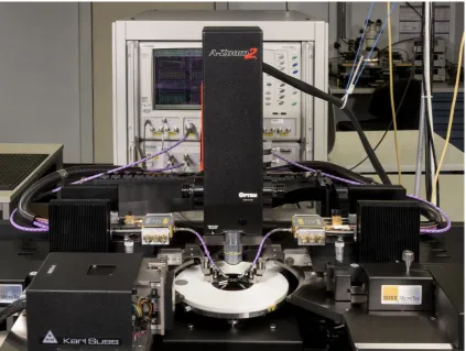
Figure 5 shows the on-wafer measurement setup used at PTB. Measurements are typically performed either on a ceramic chuck or on a metal chuck utilizing an Anritsu VectorStar VNA with mm-wave extension modules for frequencies up to 125 GHz, connected to ground-signal-ground microwave probes from various vendors with differing pitch sizes. To enable automated multiline TRL calibrations, a semi-automated wafer prober (S¨uss PA 200) with motorized x/y-positioner on the right-hand side is used.

To estimate the uncertainty contributions of the VNA, the measurement setup must be characterized. Procedures for this are given in [28] for coaxial lines and rectangular waveg-uides, and can be applied to some extent to on-wafer setups. In the following, the most relevant input quantities for the measurement process are listed with their respective values and/or uncertainties. The coverage factor is k=2 (95 % confidence level) unless indicated otherwise. Usually, the uncertainty contribution increase for higher frequency. But some-times, due to the measurement setup itself (or internal VNA architecture), large uncertainty values arise for medium or even lower frequency ranges.

1.4.1 Noise Floor/Trace Noise

(11)

Figure 5 PTB on-wafer measurement setup.

contributions are stated for k = 1. The results given in Table 1 are based on repeated measurements of two VNA ports with attached shorts.

1.4.2 Linearity

For the VNA shown in Fig. 5 the uncertainty due to not perfectly linear receiver was esti-mated to 0.01 dB and 0.066◦ for the complete magnitude and frequency range. These values can be obtained with measurements of characterized attenuation devices (often step atten-uators with very low measurement uncertainty), but good estimates are often given in the data sheet of the device manufacturer.

1.4.3 Error Term Drift

[image:11.595.95.519.41.360.2]

Drift of the measurement setup is often a major uncertainty contribution in VNA measure-ments. One can use different definitions: drift of raw values (perhaps even for different

Table 1 Uncertainties due to noise (k=1).

Frequency Noise Floor Trace Noise Trace Noise / GHz / dB Mag / dB rms Phase (◦ rms)

00.000 -110 0.004 0.03

30.000 -120 0.003 0.04

30.001 -100 0.003 0.02

55.000 -100 0.002 0.01

55.001 -115 0.001 0.01

80.000 -120 0.001 0.01

80.001 -115 0.002 0.05

120.000 -100 0.004 0.03

(12)

nominal values of the connected DUT) or drift of the calibrated setup. Here, the results are given for the drift of the error terms (of the calibrated VNA), see [28]. Table 2 shows the drift results for the VNA of Fig. 5.

Table 2 Uncertainties due to error term drift.

Frequency Switch Direc- Tracking Symmetry Match Term tivity Mag Phase Mag Phase

/ GHz / dB / dB / dB / ◦ / dB /◦ / dB 0.000 -35 -35 0.07 0.6 0.025 0.4 -35 10.000 -35 -35 0.07 0.6 0.025 0.4 -35 10.001 -35 -35 0.03 1.0 0.01 0.2 -35 20.000 -35 -35 0.03 1.0 0.01 0.2 -35 20.001 -35 -35 0.06 1.4 0.03 0.2 -35 30.000 -35 -35 0.06 1.4 0.03 0.2 -35 30.001 -50 -50 0.03 0.8 0.01 0.3 -50 120.000 -50 -50 0.03 0.8 0.01 1.1 -50

1.5 Cable Movement

If cables are moved during measurements, an uncertainty contributions must be estimated for this movement. In Fig. 5, 1-mm cables are connected to the actual on-wafer probe, but they are not moved. Moved are the cables connected to the mm-wave extension modules. The movement of the cables between the VNA and the mm-wave extensions can sometimes be neglected, because the frequency is usually low (< 20 GHz). For the setup of Fig. 5, however, the cable effects are not negligible. They were determined by repeated measuring of coaxial shorts and matched devices following the procedures from [28]. The results are given in Table 3.

Table 3 Uncertainties due to cable movement.

Frequency Reflection Transmission Transmission / GHz stability / dB stability Mag / dB stability Phase / ◦

00.000 -50 0.05 0.1

30.000 -50 0.05 0.4

30.001 -60 0.01 0.1

120.000 -60 0.01 0.1

1.6 Connection Repeatability

The uncertainty due to limited connection repeatability has been considered with -60 dB in this study. The value was determined from repeated measurements ([28]) of several on-wafer devices and is only valid for one combination of probe and substrate. One has to be careful, not to include other uncertainty contributions (e.g. drift, cable movement), thus the measurements should be done quickly enough, but without moving any cables.

1.7 DUT Uncertainty/Crosstalk

(13)

frequency as well as on the reflection magnitude of the measured device, which is substrate-dependent. It was estimated from several measurements of structures on a fused silica substrate with different reflection magnitudes and is given in Table 4.

Table 4 Transmission uncertainties due to crosstalk (in dB)

Reflection Frequency (GHz) Mag (lin. mag.) 0 20 50 120

0.0 -60 -55 -50 -45 0.2 -60 -55 -50 -45 0.8 -60 -40 -35 -20 1.0 -60 -40 -35 -20

(14)

2 On-wafer measurements up to 110 GHz

2.1 Results from a three-party on-wafer measurement

intercom-parison

In [31] we reported on initial results of a three-party on-wafer measurement intercomparison carried out on a custom-made alumina calibration substrate in the frequency range up to 110 GHz. The participants of the intercomparison were PTB, FVB, and FhG, all contributing with their individual measurement configuration. At PTB, for instance, measurements were performed VNA shown in Fig. 5 with millimetre-wave extension modules for frequencies up to 125 GHz, connected to GGB ground-signal-ground microwave probes with 100 and 150 µm pitch. The correction of the vector network analyzer measurement was performed for all participants with the highly-accurate multiline TRL calibration [5]. The focus of the investigation was on the influence of the measurement system, the probe geometry and operator skills.

2.1.1 Influence of probe pitch

The results of this first comparison showed that many factors have to be considered for the evaluation of on-wafer measurements. However, it is very difficult to isolate the factors leading to the differences observed between the different configurations. At the present state it is especially difficult to assign certain artifacts in the measurements to certain properties of the probe. Simulations indicated that main influences stem from the extension of the probe, the extension of any absorber around the probe and the extension and geometry of the needles. An important role plays also the region of the transition from the coaxial line to the needles.

As an example, Fig. 6 shows the difference between error-corrected measurements of an attenuator performed at PTB with GGB probes differing in the pitch width (100 µm versus 150 µm). The experiment was performed in a very controlled environment, using the same measurement setup, the same calibration structures, the same chuck material and, last but not least, the same operator. Nonetheless, a systematic deviation for frequencies above 50 GHz can be observed, which can almost certainly be attributed to the difference between the probe geometries. For probes from different vendors, even bigger deviations can occur.

0 10 20 30 40 50 60 70 80 90 100 110

Frequency /GHz

-16 -15.5 -15 -14.5

|S

21

|/dB

(15)

2.1.2 Importance of measurement speed/instrument drift

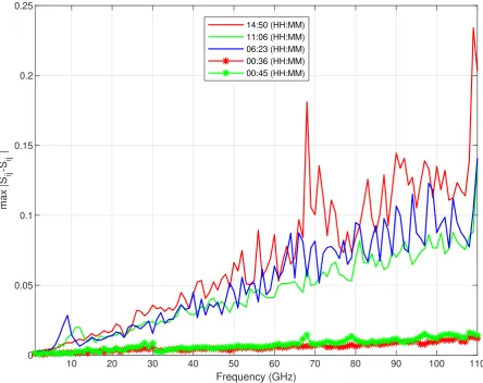
As part of the intercomparison of [31] the partners agreed on the relevant measurement parameters and system settings such as IF bandwidth, frequency range, number of data points and the calibration substrate to rule out deviations. The devices to be measured were documented in a detailed measurement plan and in order to achieve an identical evaluation with a multiline TRL calibration, all partners were encouraged to acquire raw data. The calibration substrate was circulated between the partners. Each party was allowed to choose the on-wafer probes (pitch size according to the calibration substrate), chuck material and the operator individually. Within the given parameters, the measuring speed could only be varied by the on-wafer prober station (automatic / manual) and by the operator.

Within this three-party on-wafer measurement intercomparison a total of eleven datasets with different settings were evaluated. An essential result of the evaluation was that not the on-wafer prober type (semi automated / manual station) showed the biggest influence on the calibration results, but the operator with the overall measurement time. Artefacts caused by system drift and stability could be identified from the data resulting from longer measurement durations. In order to obtain reliable measurement results the operator should therefore try to measure with a continuously fast speed, this applies for the calibration standards as well as the DUTs. With a short overall measurement duration and a fast measurement process the system/instrument drift influence can be reduced significantly (see Fig. 7).

10 20 30 40 50 60 70 80 90 100 110

Frequency (GHz)

0 0.05 0.1 0.15 0.2 0.25

max |S

ij

-S

ij

´|

14:50 (HH:MM) 11:06 (HH:MM) 06:23 (HH:MM) 00:36 (HH:MM) 00:45 (HH:MM)

Figure 7 Drift as a function of measurement duration calculated as worst-case error bounds with the method of [32] (HH:MM is the total measurement time in hours:minutes).

[image:15.595.81.526.354.706.2]

(16)

2.2 Limits of established techniques for transferring uncertainties

In this section we report on methods to transfer uncertainties from reference calibration substrates to working calibration substrates. The aim is to preserve the low uncertainties in S-parameter measurements achieved on custom-made reference calibration substrates even when using low-cost working calibration substrates, such as e.g. impedance standard sub-strates, which can be purchased from several on-wafer vendors. Recommendations for the transfer of uncertainties will be given at the end of the section.

2.2.1 Substrate permittivity compensation

In [33], a simple capacitance model was developed to account for the effect of a change in substrate permittivity on coplanar waveguide TRL calibrations performed on different substrate materials. For all calibrations, the reference plane was moved to the probe tip and the reference impedance was set to 50 Ω. Whereas in [33] all cross-sectional dimensions of the CPWs on the different substrates were assumed identical, the investigation in [34] demonstrated that also the measurement error caused by differences in the conductor geom-etry can be accounted for. As the measurements in [33] and in [34] were limited to the 40 GHz frequency range, we investigated the performance of this compensation technique using custom-made fused silica and Al2O3 substrates up to 110 GHz.

0 10 20 30 40 50 60 70 80 90 100 110

Frequency (GHz)

0 0.05 0.1 0.15 0.2 0.25

Upper bound on |S

ij

-S

ij

)|

Silica MTRL 50 Ohm vs. Al2O3 MTRL 50 Ohm

[image:16.595.83.530.332.651.2]

Silica MTRL 50 Ohm vs. Al2O3 MTRL 50 Ohm /w permittivity compensation

Figure 8 Worst-case error bounds calculated by calibration comparison method [32].

(17)

To this end, we investigated measurements of different devices fabricated on the Al2O3

wafer in the frequency range from 1 to 110 GHz (see Figs. 9-13). The multiline TRL cali-bration on the Al2O3 wafer gives the most accurate result (black curves), while the multiline

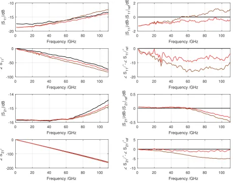
TRL calibration on the fused silica wafer (brown curves) will introduce a systematic error due to the differences in substrate permittivity and conductor geometries. The red curves show the result for the multiline TRL calibration on the fused silica wafer after applying the substrate permittivity compensation technique of [33]. In the following figures, the error-corrected reflection and transmission measurement are shown on the left-hand side, while the differences with regard to the reference calibration are shown on the right-hand side. In the case of one-port devices only the results for reflection are shown.

In Fig. 9, the results for an attenuator device are displayed. While the permittivity compensation only slightly improves the error in magnitude ofS11andS21, there is a tangible

improvement in the phase over the entire frequency range. For frequencies above 60 GHz, the errors in the magnitude of S21 cannot be compensated by the simple capacitance model

of [33].

Figure 10 shows the results for a 11.4 mm long CPW line on Al2O3 substrate. For S11,

the permittivity compensation does not offer any notable improvement over the fused silica calibration. In the phase of S21, there is a tangible improvement over the entire frequency

[image:17.595.79.538.384.744.2]

range.

Figure 11 shows the results for a mismatched CPW line on Al2O3 substrate. Here, the

permittivity compensation leads to an improvement in both S11 and S21. As is evident

from the left-hand side, the resonance frequencies of the black and red curve line up after

0 20 40 60 80 100

Frequency /GHz -20 -15 -10 |S 11 |/dB

0 20 40 60 80 100

Frequency /GHz -2 0 2 |S 11 |/dB-|S 11 |ref /dB

0 20 40 60 80 100

Frequency /GHz -100 -50 0 S 11 / °

0 20 40 60 80 100

Frequency /GHz -20 -10 0 S 11 / ° S 11 / ° ref

0 20 40 60 80 100

Frequency /GHz -16 -15 -14 |S 21 |/dB

0 20 40 60 80 100

Frequency /GHz -0.5 0 0.5 |S 21 |/dB-|S 21 |ref /dB

0 20 40 60 80 100

Frequency /GHz -200 -100 0 S 21 / °

0 20 40 60 80 100

Frequency /GHz -10 -5 0 5 S 21 / ° S 21 / ° ref

Figure 9 left: reflection and transmission measurement of attenuator device on Al2O3 substrate

right: measurement normalized to MTRL result on Al2O3

colors: MTRL on Al2O3 (black),on fused silica, on fused silica after perm. comp.

(18)

0 20 40 60 80 100 Frequency /GHz -60 -40 -20 0 |S 11 |/dB

0 20 40 60 80 100

Frequency /GHz -20 0 20 40 |S 11 |/dB-|S 11 |ref /dB

0 20 40 60 80 100

Frequency /GHz -400 -200 0 200 S 11 / °

0 20 40 60 80 100

Frequency /GHz -4 -2 0 |S 21 |/dB

0 20 40 60 80 100

Frequency /GHz -0.4 -0.2 0 0.2 |S 21 |/dB-|S 21 |ref /dB

0 20 40 60 80 100

Frequency /GHz -400 -200 0 200 S 21 / °

0 20 40 60 80 100

[image:18.595.79.538.46.405.2]

Frequency /GHz -5 0 5 S 21 / ° S 21 / ° ref

Figure 10 left: reflection and transmission measurement of 11.4 mm long CPW line on Al2O3

applying the compensation. Again, the corrective effect of the permittivity compensation is more noteable in the phase, and for frequencies above 60 GHz, the errors in the magnitude of S21 cannot be compensated by the technique of [33].

Figure 12 shows the results for a one-port device, an offset open. The permittivity compensation only improves the phase of S11. The compensation does not work for the

magnitude of S11, and again, for frequencies above 60 GHz, the systematic errors in the

magnitude of S11 start to increase with frequency.

Figure 13 shows the results for a 0.4 mm long thru line on Al2O3 substrate. For S11,

the permittivity compensation hardly offers any improvement over the fused silica calibra-tion. There is a tangible improvement in the phase of S21 over the entire frequency range.

For frequencies above 60 GHz, the systematic errors in the magnitude of S21 cannot be

compensated by the technique of [33].

In summary, one can state the permittivity compensation technique of [33] mostly im-proves on the phase error introduced by the off-wafer calibration on fused silica. The effect is generally more noteable in S21 compared to S11. With regard to the magnitude error,

which drastically increases for frequencies above 60 GHz in S21, almost no improvement can

(19)

0 20 40 60 80 100 Frequency /GHz -60 -40 -20 0 |S 11 |/dB

0 20 40 60 80 100

Frequency /GHz -20 -10 0 10 |S 11 |/dB-|S 11 |ref /dB

0 20 40 60 80 100

Frequency /GHz -100 0 100 S 11 / °

0 20 40 60 80 100

Frequency /GHz -2 -1 0 |S 21 |/dB

0 20 40 60 80 100

Frequency /GHz -400 -200 0 200 S 21 / °

0 20 40 60 80 100

Figure 11 left: reflection and transmission measurement of mismatched line on Al2O3

0 20 40 60 80 100

Frequency /GHz -1 -0.5 0 0.5 |S 11 |/dB

0 20 40 60 80 100

Frequency /GHz -150 -100 -50 0 S 11 / °

0 20 40 60 80 100

Frequency /GHz -80 -60 -40 -20 |S 21 |/dB

0 20 40 60 80 100

Frequency /GHz -2 -1 0 1 |S 21 |/dB-|S 21 |ref /dB

0 20 40 60 80 100

Frequency /GHz -400 -200 0 200 S 21 / °

0 20 40 60 80 100

[image:19.595.76.534.73.430.2]

Frequency /GHz -6 -4 -2 0 S 21 / ° S 21 / ° ref

Figure 12 left: reflection and transmission measurement of open device on Al2O3

(20)

0 20 40 60 80 100 Frequency /GHz -80 -60 -40 -20 |S 11 |/dB

0 20 40 60 80 100

Frequency /GHz -400 -200 0 200 S 11 / °

0 20 40 60 80 100

Frequency /GHz -0.4 -0.2 0 0.2 |S 21 |/dB

0 20 40 60 80 100

Frequency /GHz -150 -100 -50 0 S 21 / °

0 20 40 60 80 100

[image:20.595.77.533.219.579.2]

Frequency /GHz -5 0 5 S 21 / ° S 21 / ° ref

Figure 13 left: reflection and transmission measurement of thru line on Al2O3

(21)

2.2.2 Residual error correction

A more general approach for compensating systematic errors introduced by the VNA cali-bration is the determination of residual errors and the application of a second-order error correction afterwards. In [35], a method for determining complex residual errors of two-port VNA calibrations was presented which makes use of a time-domain approach. The resid-ual errors are extracted from a distance-frequency system model using a special estimation algorithm based on the quasi-optimal unscented Kalman filter. Since the method requires only three measurement conditions, it is particularly suited for on-wafer applications, as these conditions can be obtained from using only one verification line. In [36], the same measurement conditions are exploited, but since the residual error terms are now estimated by applying a least-mean-squares method the calculation time is significantly reduced.

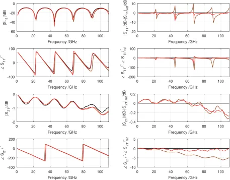
Here, we determined the residual errors of calibrated two-port on-wafer measurements up to 110 GHz with the method of [36], utilizing the commercial calibration substrate GGB CS5 and GGB100 microwave probes. As verification line, line 10 with a length of 6600 µm was used. As DUTs lines of different lengths were used. By analyzing the error-corrected mea-surements of the DUTs, we compared the accuracy of SOLT calibrations with characterized standards to SOLT calibrations with manufacturer definitions and to second-order-corrected SOLT calibrations with manufacturer definitions. In the following figures, the error-corrected reflection and transmission measurement are shown on the left-hand side, while the differ-ences with regard to the reference calibration (SOLT with characterized standards) are shown on the right-hand side.

Figures 14-16 show the results for lines with lengths in the range 550. . .1500 µm. One obvious disadvantage of the second-order error correction becomes apparent for frequen-cies below 10 GHz: additional errors are introduced leading to unphysical behavior in both reflection and transmission. For higher frequencies, however, the second-order correction is mostly working as expected. In the measured reflections, the second-order error correction is beneficial in both magnitude and phase, as can be seen from the red S11curves approaching

the black S11 curves in a range of approximately 20. . .110 GHz. In the measured

transmis-sion, there is almost no improvement for the magnitude of S21, while the phase ofS21 even

deteriorates slightly by means of the second-order error correction.

In summary one can state that the second-order error correction of [36] shows some promise but is currently limited by the accuracy with which the residual errors can be determined. At the edges of the frequency range (ca. 5% of the frequency band), the error of the filtering algorithm increases. This applies to measurements of both transmission and reflection coefficients. In principle, the effect can be reduced by applying a verification line with a longer length.

The current study was limited by the number of DUTs and the verification line available on the commercial calibration substrate. Future investigations should try to extend the study to better understand and overcome the current limitations of the method of [36].

(22)

0 20 40 60 80 100 Frequency /GHz -80 -60 -40 -20 |S 11 |/dB

0 20 40 60 80 100

Frequency /GHz -400 -200 0 200 S 11 / °

0 20 40 60 80 100

Frequency /GHz -0.4 -0.2 0 0.2 |S 21 |/dB

0 20 40 60 80 100

Frequency /GHz -200 -100 0 S 21 / °

0 20 40 60 80 100

[image:22.595.72.536.215.569.2]

Figure 14 left: SOLT-corrected reflection and transmission of 550µm long line on GGB CS5 right: measurement normalized to SOLT with characterized standards

colors: characterized standards (black), manufacturer definitions, manufacturer

(23)

0 20 40 60 80 100 Frequency /GHz -60 -40 -20 |S 11 |/dB

0 20 40 60 80 100

Frequency /GHz -400 -200 0 200 S 11 / °

0 20 40 60 80 100

Frequency /GHz -0.5 0 0.5 |S 21 |/dB

0 20 40 60 80 100

Frequency /GHz -400 -200 0 200 S 21 / °

0 20 40 60 80 100

[image:23.595.75.536.213.569.2]

defi-nitions after residual error correction

(24)

0 20 40 60 80 100 Frequency /GHz -60 -40 -20 |S 11 |/dB

0 20 40 60 80 100

Frequency /GHz -400 -200 0 200 S 11 / °

0 20 40 60 80 100

Frequency /GHz -1 -0.5 0 0.5 |S 21 |/dB

0 20 40 60 80 100

Frequency /GHz -400 -200 0 200 S 21 / °

0 20 40 60 80 100

[image:24.595.73.536.213.569.2]

(25)

2.3 Transfer of uncertainties with the aid of ISS

In [22] it was demonstrated that properly characterized standards can be used to account for differences between the commercial ISS and the target DUT measurement situation. The results of a reference MTRL calibration using custom standards were in essence duplicated with the aid of characterized ISS standards and a much simpler calibration, in this case SOLT. This constitutes a big improvement over any of the approaches discussed in the two previous subsections, where a systematic error with regard to the reference result remained. Therefore, in order to transfer uncertainties to industrial applications where commercial ISS substrates and simple calibration algorithms have to be used, one has to first characterize the standards in a manner which is adequate for the target application. This requires building custom calibration standards on the target DUT wafer, which serve for characterizing the ISS calibration standards appropriately. In the following, we demonstrate this approach with the custom-made Al2O3 wafer as the target DUT wafer and the GGB CS5 calibration

substrate as commercially available ISS substrate.

Recently, PTB developed a traceability path for on-wafer S-parameter measurements based on the MTRL calibration algorithm [10]. The methodology of [10] for establishing a comprehensive uncertainty budget can also be applied to other substrates, as long as the wideband material properties are known and single-mode propagation can be assumed. For the custom-made Al2O3 wafer used in our studies, the latter condition is strictly fulfilled

only for frequencies below ca. 70 GHz. For higher frequencies, the effects of dispersion and interaction with higher-order and other parasitic modes are currently not fully captured in the uncertainty budget. Nonetheless we used this preliminary uncertainty budget and treated the Al2O3 wafer as reference calibration wafer for characterizing the standards on

the GGB CS5 substrate.

Figures 17 and 18 show the result of characterizing the Open/Short/Load/Thru stan-dards by means of a reference multiline TRL calibration on the custom-made Al2O3 wafer.

The figures also show the expanded uncertainty intervals comprising the influences of MTRL calibration standard uncertainties, uncertainties from the instrumentation used, cabling in-fluences and repeatability effects. It may appear surprising that some of the characterized standards show gain even though they are passive devices. This can easily be explained by the fact that the distance between the probe tips on the CS5 standards was smaller than the distance between the calibration reference planes on the Al2O3 wafer. Nonetheless the

char-acterized CS5 standards can be used as transfer standards for accurately measuring DUTs on the Al2O3 wafer.

Fig. 19 compares the measurement results for an attenuator DUT and a mismatched line DUT fabricated on the Al2O3 wafer. The black curves show the reflection and transmission

when using the reference MTRL calibration on the Al2O3 substrate, the red curves show the

corresponding results for the SOLT calibration with the characterized CS5 standards. The shaded areas indicate the expanded uncertainty intervals. It can be clearly seen that the nominal values coincide for both calibrations, proving the consistency of the approach. The only differences appear in the expanded uncertainties, which are usually slightly increased for the calibration with the characterized standards.

Exemplary uncertainty budget values for the DUTs corrected via the SOLT calibration with characterized CS5 standards are given in the Tables 5-8. These tables show the uncer-tainty budget composition for the magnitude of S11 and the phase of S21 of the DUTs at a

frequency of 65 GHz. The calibration standard uncertainties are designated with PTB ML in the beginning, pointing to the fact that the characterization was performed with the PTB multiline calibration. The tables clearly show that the budgets are mostly dominated by the calibration standard uncertainties. For the phase of S21, also cable effects and DUT

uncertainty provide significant contributions to the total uncertainty at 65 GHz.

(26)

0 20 40 60 80 100 Frequency /GHz 0.98 1 1.02 1.04 |S 11 |

0 20 40 60 80 100

Frequency /GHz 0.98 1 1.02 1.04 |S 11 |

0 20 40 60 80 100

Frequency /GHz -20 -10 0 S 11 / °

0 20 40 60 80 100

Frequency /GHz 172 174 176 178 180 S 11 / °

0 20 40 60 80 100

Frequency /GHz 0 0.05 0.1 |S 21 |

0 20 40 60 80 100

Frequency /GHz 0 0.05 0.1 |S 21 |

0 20 40 60 80 100

Frequency /GHz -100 0 100 S 21 / °

0 20 40 60 80 100

[image:26.595.75.537.226.579.2]

Frequency /GHz 0 100 200 300 S 21 / °

(27)

0 20 40 60 80 100 Frequency /GHz 0 0.02 0.04 0.06 0.08 |S 11 |

0 20 40 60 80 100

Frequency /GHz -0.02 0 0.02 0.04 |S 11 |

0 20 40 60 80 100

Frequency /GHz -200 -100 0 S 11 / °

0 20 40 60 80 100

Frequency /GHz -200 0 200 S 11 / °

0 20 40 60 80 100

Frequency /GHz 0 0.01 0.02 |S 21 |

0 20 40 60 80 100

Frequency /GHz 0.98 1 1.02 |S 21 |

0 20 40 60 80 100

Frequency /GHz 0 100 200 S 21 / °

0 20 40 60 80 100

[image:27.595.78.538.227.584.2]

Frequency /GHz -40 -30 -20 -10 S 21 / °

Figure 18 left: characterized Load standard on GGB CS5 substrate; right: characterized Thru standard on GGB CS5 substrate.

(28)

0 20 40 60 80 100 Frequency /GHz 0.1 0.15 0.2 |S 11 |

0 20 40 60 80 100

Frequency /GHz 0 0.1 0.2 0.3 |S 11 |

0 20 40 60 80 100

Frequency /GHz -80 -60 -40 -20 0 S 11 / °

0 20 40 60 80 100

Frequency /GHz -100 0 100 200 S 11 / °

0 20 40 60 80 100

Frequency /GHz 0.16 0.17 0.18 0.19 |S 21 |

0 20 40 60 80 100

Frequency /GHz 0.85 0.9 0.95 |S 21 |

0 20 40 60 80 100

Frequency /GHz -150 -100 -50 S 21 / °

0 20 40 60 80 100

[image:28.595.76.536.221.572.2]

Frequency /GHz -100 0 100 S 21 / °

Figure 19 left: reflection and transmission measurement of attenuator on Al2O3

right: reflection and transmission measurement of mismatched line on Al2O3

(29)

[image:29.595.119.493.77.365.2]

Table 5 Uncertainty budget for magnitude ofS11 of attenuator at 65 GHz (in dB) .

Description Unc Component Unc Percentage

Cable Stability 0.001450124 0.000 Calibration Standards: 0.670126203 99.592

⇒ PTB ML CS5 open 51 S11 0.058003624 0.746

⇒ PTB ML CS5 open 51 S22 0.001496587 0.000

⇒ PTB ML CS5 res 71 50 S11 0.666248662 98.443

⇒ PTB ML CS5 res 71 50 S22 0.002807877 0.002

⇒ PTB ML CS5 short 61 S11 0.038046580 0.321

⇒ PTB ML CS5 short 61 S22 0.001042205 0.000

⇒ PTB ML CS5 thr 81 S11 0.018936710 0.080

⇒ PTB ML CS5 thr 81 S12 0.000143966 0.000

⇒ PTB ML CS5 thr 81 S21 0.000143964 0.000

⇒ PTB ML CS5 thr 81 S22 0.000184802 0.000 Connector Repeatability 0.039950930 0.354 DUT Uncertainty 0.000055924 0.000 VNA Drift (Ideal VNA correlated) 0.015253581 0.052

VNA Linearity 0.000000000 0.000

VNA Noise 0.002606109 0.002

Value: -16.245 Std Unc: 0.671 U95: 1.342

Table 6 Uncertainty budget for phase of S21 of attenuator at 65 GHz (in ◦) .

⇒ PTB ML CS5 open 51 S11 0.232294374 2.077

⇒ PTB ML CS5 open 51 S22 0.020862472 0.017

⇒ PTB ML CS5 res 71 50 S11 0.140175758 0.756

⇒ PTB ML CS5 res 71 50 S22 0.083127246 0.266

⇒ PTB ML CS5 short 61 S11 0.168673048 1.095

⇒ PTB ML CS5 short 61 S22 0.014458089 0.008

⇒ PTB ML CS5 thr 81 S11 0.114784009 0.507

⇒ PTB ML CS5 thr 81 S12 0.025697228 0.025

⇒ PTB ML CS5 thr 81 S21 1.232926518 58.497

VNA Linearity 0.000000000 0.000

VNA Noise 0.018006836 0.012

Value: -90.9098 Std Unc: 1.612 U95: 3.224

[image:29.595.116.492.412.700.2]

(30)

[image:30.595.119.493.76.365.2]

Table 7 Uncertainty budget for magnitude of S11 of mismatched line at 65 GHz (in dB) .

⇒ PTB ML CS5 open 51 S11 0.023740527 0.014

⇒ PTB ML CS5 open 51 S22 0.070263207 0.118

⇒ PTB ML CS5 res 71 50 S11 1.883437737 85.000

⇒ PTB ML CS5 res 71 50 S22 0.125927050 0.380

⇒ PTB ML CS5 short 61 S11 0.049882933 0.060

⇒ PTB ML CS5 short 61 S22 0.058699120 0.083

⇒ PTB ML CS5 thr 81 S11 0.763456399 13.966

⇒ PTB ML CS5 thr 81 S12 0.006792718 0.001

⇒ PTB ML CS5 thr 81 S21 0.006792700 0.001

VNA Linearity 0.000000000 0.000

VNA Noise 0.011795602 0.003

Value: -19.804 Std Unc: 2.043 U95: 4.086

Table 8 Uncertainty budget for phase of S21 of mismatched line at 65 GHz (in ◦) .

⇒ PTB ML CS5 open 51 S11 0.192502364 1.546

⇒ PTB ML CS5 open 51 S22 0.008051523 0.003

⇒ PTB ML CS5 res 71 50 S11 0.360163455 5.413

⇒ PTB ML CS5 res 71 50 S22 0.296612500 3.671

⇒ PTB ML CS5 short 61 S11 0.149293085 0.930

⇒ PTB ML CS5 short 61 S22 0.015031594 0.009

⇒ PTB ML CS5 thr 81 S11 0.075873173 0.240

⇒ PTB ML CS5 thr 81 S12 0.011439288 0.005

⇒ PTB ML CS5 thr 81 S21 1.247369834 64.922

VNA Linearity 0.000000000 0.000

VNA Noise 0.018249220 0.014

[image:30.595.114.494.411.701.2]

(31)

3 On-wafer measurements above 110 GHz

3.1 Recommended good practice for making on-wafer

measure-ments at higher frequencies

The subject of recommended good practice for making on-wafer measurements above 110 GHz is still relatively new. One reason for this is that the hardware for making such mea-surements has been either scarce or not available at all. However, this situation has been changing in recent years, particularly with VNA extender heads becoming available at these frequencies. In fact, these extender heads are now commercially available at all frequencies to at least 1 THz.

The rollout of these VNA extender heads has been closely followed by the availability of on-wafer probes and calibration standards (on-wafer impedance standard substrates). The current state of the art is S-parameter measurements at all frequencies to 1.1 THz. However, there is very little published information available of the use of this on-wafer hardware at these frequencies – particularly, with regard to determining the quality and reliability of on-wafer measurements obtained at these frequencies.

The recently completed European research project, PlanarCal [1], has been a very valu-able resource in this respect. This project included a substantial amount of work looking at making on-wafer measurements above 110 GHz. In this work, it was first noted that metrological traceability, as defined in [37], for on-wafer measurements above 110 GHz is not currently available anywhere in the world. Traditionally, it is the role of National Measure-ments Institutes (NMIs) such as PTB (Germany), NPL (UK), etc, to make available facilities that provide metrological traceability to end-users in industry and elsewhere. However, to establish such capabilities usually requires a large sustained effort – such an effort has yet to be made, by the NMI community, with regard to on-wafer measurements above 110 GHz.

When traceability does exist, it is relatively straightforward for end-users to determine the quality and reliability of measurements, simply by comparing their measurements with traceable references coming from the NMI community. These NMI measurements are ul-timately linked back to the base units of the International System of units (SI). However, when traceability does not exist (as is the case for on-wafer measurements above 110 GHz), it is often useful for measurement laboratories to undertake repeatability and reproducibil-ity studies in order to determine the main sources of variabilreproducibil-ity (and hence the qualreproducibil-ity, reliability, etc) in such measurements [38].

Some preliminary studies of repeatability and reproducibility have been conducted during the PlanarCal project [39, 40]. These studies involved the participating laboratories in making measurements using their usual measurement setups – i.e. VNA/extender heads, probe stations, on-wafer probes, calibration techniques, calibration substrates and calibration standards. The different choices of these aspects of the measurement process help to expose the effect these aspects have on the measurement results that are obtained during the study. Different probe designs will interact with the calibration substrate to produce parasitic elements that may not be the same as those on the DUT wafer, leading to systematic errors [41]. At higher millimetre-wave frequencies, the ground-signal-ground (GSG) probe pitch can become an appreciable fraction of the signal wavelength [42]. The use of GSG pitches of 75 µm or less is recommended.

Other major issues with measurements at high millimetre-wave frequencies and above concern isolation/crosstalk, the presence of parasitic modes (e.g. higher-order modes and substrate modes) and the effects due to neighbouring structures (i.e. other components) found close to the calibration standards on the calibration wafer. These issues were also investigated during the PlanarCal project. Some of the outcomes from these investigations have been reported in [43].

Coplanar waveguide structures, such as those typically fabricated on DUT wafers, will

(32)

exhibit higher-order modes above 50 GHz, depending on the boundary conditions above and below the substrate. It is good practice to use an absorbing material (with similar dielectric constant as the substrate) between the metallic wafer chuck and the DUT, which will suppress unwanted modes. The DUT is effectively a different structure (electromagnetically) with and without this absorber, and measurement results can differ widely depending on whether or not it is used.

Sometimes the presence of systematic errors in the measurements can be detected espe-cially when non-physical behaviour is observed – e.g. when the observed linear magnitude of the reflection coefficient is greater than unity. This is indicative of an inappropriate reference standard used during calibration. Additionally, the presence of significant ripple on some measurement traces suggest perhaps the use of an inferior calibration technique. Generally, the choice of reference calibration substrate can have a major impact on the achieved measurements. This is because the different calibration substrates provide differ-ent calibration reference values (e.g. due to the use of differdiffer-ent substrate materials for the calibration substrate). This means that even the same uncorrected measurement data for a given device under test (DUT) will give rise to different corrected S-parameter values due to different reference values being used during the calibration process. This occurs when a VNA is calibrated using standards found on one wafer (e.g. a commercial impedance stan-dard substrate), and then measurements are made subsequently of DUTs on another wafer (e.g. the wafer containing the devices that need testing). For this reason, when making on-wafer S-parameter measurements that are not SI traceable, it is very important to state what references were used during calibration. In fact, as a general rule, it is good practise to state everything about the measurement setup that might have an impact on the obtained measurement results – e.g. VNA, probes (including probe pitch) and associated calibra-tion hardware and software (i.e. the calibracalibra-tion substrate, the calibracalibra-tion method and the calibration standards used).

Whenever possible, it is preferable to fabricate some appropriate reference standards on the same wafer as the DUT. As a minimum, some lengths of CPW line and some high-reflecting standards (usually short-circuits) are needed. These enable the use of one of the calibration techniques derived from the TRL approach [44, 5] which make use of the CPW lines to acquire a reference value which is determined by the properties of the DUT substrate material. These techniques are generally superior to the more conventional Short-Open-Load-Thru (SOLT) technique, and are less dependent on accurate and repeatable probe-placement. For manual probe stations, this can be a significant source of error at higher frequencies if the calibration method requires known values for the phase of the calibration standards.

3.2 Summary of high-frequency parasitic effects

When operating in the mm-wave frequency range (i.e., in the context of this section above 110 GHz), the calibration errors arising from the inaccuracy of standard models and mul-timode propagation start to severely impact the calibration accuracy that can be achieved. For this reason a guideline to inform the reader on these potential problems and the means to minimize them was compiled in the EMPIR PlanarCal project, namely, “Guidelines for the design of calibration substrates, including the suppression of parasitic modes for frequen-cies up to and including 325 GHz ”. The interested reader is invited to familiarize himself with these effects using the above mentioned document. In the following a selection of the suggestions provided in the document is given:

Choice of substrate thickness (Guideline #1)

Compute the critical frequency (fc) of parasitic modes (e.g. higher order modes and substrate

(33)

or dielectric chuck) and select those in which fc is outside the calibration frequency or only

occurs in the upper calibration range, to avoid excessive coupling of power to unwanted modes.

Impact of ground-to-ground spacing in CPWs (Guideline #4)

The influences of CPW ground width and of ground-to-ground spacing, are contributing to parasitic effects in the calibrated results, in this case a dip in S-parameters at a certain frequency. Total CPW width determines the frequency where this dip occurs, and ground-to-ground spacing influences the strength of the dip behavior. Thus, the best way to mitigate the impact of this dip is to keep the total CPW width smaller than the formula given in [45], which requires a tradeoff between the CPW total width, the used material and the upper frequency limit fmax.

Chuck topology (Guideline #5)

Using for the chuck a material which has a permittivity value similar to the calibration substrate reduces the effects which contribute to the degradation of the accuracy of CPW mTRL calibrations. Further investigations have shown that this is true also for a chuck material with a permittivity larger than that of the wafer, because such a layered structure does not support surface waves either.

Influence of in-line and side-way neighbouring structures (Guideline #6)

One should keep sensitive regions of the probe shadow free of structures to avoid probe coupling to neighboring structures, as shown in the figure below (investigations performed up to 70 GHz).

Custom designed TRL kit (Guideline #8)

When designing custom kits for LRM/TRL calibration the reflect should be realized as an offset one, keeping the minimum distance between the effective reflect and the center of the thru line (intrinsic calibration plane) to avoid requiring sign changes in the solution of the calibration equations.

3.3 Surface roughness effects

Surface roughness is one among different parasitic effects that affect signal integrity of prop-agating signals on transmission lines. While radiation mainly increases the attenuation α, dispersion effects have a direct influence on the phase velocity vph and only indirectly affect

attenuation by increasing the line capacitance and thus, dielectric loss. In contrast thereto, surface roughness has shown to directly impacting on both, attenuation and phase velocity. The impact magnitude depends on the actual roughness on the one hand and the opera-tion frequency on the other. Although it is a an inevitable property of real surfaces and can be appropriately taken into account by modeling and simulation, for many practical applications an impact of only little surface roughness causing deviations between rough and

(34)

smooth responses within <5 % in attenuation α and <0.5 % in phase coefficient β may be considered as negligible.

Table 9 Frequency Bands and Waveguide Definitions.

Band Waveguide Frequency Limits W WR10 75−110 GHz

F WR08 90−140 GHz D WR06 110−170 GHz G WR05 140−220 GHz Y WR04 170−260 GHz Y WR03 220−325 GHz Y WR02 325−500 GHz Y WR01.5 500−750 GHz

For this purpose, this section provides margins for the root-mean-square (RMS) roughness

Rq which meet these requirements over the frequency bands from W- to Y-Band as shown

in Table 9 in terms of both, a general consideration and specific application to certain transmission lines.

−0.4 −0.3 −0.2 −0.1 0 0.1 0.2 0.3 0.4 0.5 0.6 0.7 0.8 0.9 1 0

0.2 0.4 0.6 0.8 1

depthx (µm)

Normalized

σ

and

H

σ(x)/σDC=CDFˆ |B0,ideal| |B0,rough|

Figure 20 Conductivity profile and skin effect on smooth and rough surface at 50 GHz with

Rq = 1µm

By making use of the Gradient Model [46], the penetrating magnetic field can be cal-culated for a given surface which is represented either by a measured bearing area curve (BAC) or Rq as shown in Fig. 20. As explained in [46], these responses may be used to

de-rive effective material parameters which in turn account for the impact of surface roughness in transmission line models such as e.g. [45] for a CPW or [47] for rectangular waveguides (RWG).

While the magnitude and ratio of surface roughness impact on α and vph depend on

the type, specific cross section geometry and materials of the transmission line, the sur-face impedance as described in [46] provides an independent approach for illustration and comparison:

Z = 1

σeffδ(σeff)

+j 1 σDCδ(µr,eff)

=

r

πµ0µrf

σeff

+j r

πµ0µr,efff

σDC

=R+jωLi, (1)

where σDC is the bulk conductivity as a material property of the conductor (e.g. 58 MS/m

(35)

parameter values derived from the Gradient Model approach which represent the impact of surface roughness. While the real part of Z affects the attenuation and is therefore related toR, its imaginary part influences vph and is related toLi,, which is the inner inductance.

0 2 4 6 8 10 12 14 16 18 20 22 24 26 28 30 32 34 36 38 40 0

5 10 15 20 25

Rq (nm)

∆

<

{

Z

}

(%)

110 GHz 140 GHz 170 GHz 220 GHz 260 GHz 325 GHz 500 GHz 750 GHz

Figure 21 Relative deviation ∆< {Z}between rough and smooth case in %

0 2 4 6 8 10 12 14 16 18 20 22 24 26 28 30 32 34 36 38 40 0

100 200 300 400

Rq (nm)

∆

=

{

Z

}

(%)

110 GHz 140 GHz 170 GHz 220 GHz 260 GHz 325 GHz 500 GHz 750 GHz

Figure 22 Relative deviation ∆= {Z}between rough and smooth case in %

Figs. 21 and 22 show the relative deviation between the rough and smoothZ depending on Rq for the considered frequency band limits. From the real part, a 5 % margin can

therefore be derived for each band, indicating the need for lowerRqwith increasing operation

frequencies.

Although the deviation within the imaginary part of Z in Fig. 22 exceeds 100 % for relatively small Rq already, it is worth to mention, that it only contributes to the inner

inductance term Li which is much smaller than the outer inductance Lo (Li Lo) and

is therefore only a fraction of the total inductance for most practical transmission lines. Furthermore, the 5 % limit in < {Z} is not directly related to the attenuation of a specific transmission line, since the conductor circumference must be considered according to the cross section geometry [48].

While the layout of a CPW allows for various implementations depending on the substrate material, manufacturing aspects and others, rectangular waveguides are typically produced

(36)

in standardized dimensions according to their identifier WR-XX in Table 9. This allows for precise predictions of the surface roughness impact which is shown in Figs. 23 and 24.

0 5 10 15 20 25 30 35 40 45 50

0 5 10 15 20

Rq (nm)

∆

α

(%)

WR10 WR08 WR06 WR05 WR04 WR03 WR02 WR01.5

Figure 23 Relative deviation ∆α between rough and smooth RWG in %.

0 5 10 15 20 25 30 35 40 45 50

0 2 4 6 8 10

Rq (nm)

∆

β

(

o /o

o

)

WR10 WR08 WR06 WR05 WR04 WR03 WR02 WR01.5

Figure 24 Relative deviation ∆β between rough and smooth RWG ino_/ oo.

Note, that the deviation in β is provided in o_/

oo as it is rather small as compared to the

impact on α. However, it comes along with a small shift of the cutoff frequency fc towards

lower values.

TheRq-margins for CPWs can be provided for certain cases only, since CPW lines can be

fabricated in a much greater variety compared to standardized RWG. Exemplarily, a CPW implemented on Al2O3 substrate (εr= 9.7) is considered with the cross section geometry as

provided in Fig. 25.

In addition to the phase coefficientβ, in this case, also the effective relative permittivity is considered according to:

εr,eff=

c0

vph

2

(2)

The corresponding Rq margins are provided in Figs. 26 to 31 for attenuation and phase

(37)

wc= 50µm

wg = 270µm wg = 270µm

s= 25µm

s= 25µm t = 5µm

h

Figure 25 Cross section geometry of a CPW structure as considered in this comparison.

10 12 14 16 18 20 22 24 26 28 30 32 34 36 38 40 42 44 46 48 50 0

5 10 15

Rq (nm)

∆

α

(%)

110 GHz 140 GHz 170 GHz 220 GHz 260 GHz 325 GHz

Figure 26 Relative deviation ∆α between rough and smooth CPW in % for h= 100µm.

10 12 14 16 18 20 22 24 26 28 30 32 34 36 38 40 42 44 46 48 50 0.2

0.4 0.6 0.8 1

Rq (nm)

∆

β

(%)

Figure 27 Relative deviation ∆β between rough and smooth CPW in % for h= 100µm.

(38)

10 12 14 16 18 20 22 24 26 28 30 32 34 36 38 40 42 44 46 48 50 0.5

1 1.5 2

Rq (nm)

∆

εr,eff

(%)

Figure 28 Relative deviation ∆εr,eff between rough and smooth CPW in % for h= 100µm.

10 12 14 16 18 20 22 24 26 28 30 32 34 36 38 40 42 44 46 48 50 0

2 4 6

Rq (nm)

∆

α

(%)

110 GHz 140 GHz

Figure 29 Relative deviation ∆α between rough and smooth CPW in % for h= 10 mm.

10 12 14 16 18 20 22 24 26 28 30 32 34 36 38 40 42 44 46 48 50 0.2

0.4 0.6 0.8 1

Rq (nm)

∆

β

(%)

110 GHz 140 GHz

(39)

10 12 14 16 18 20 22 24 26 28 30 32 34 36 38 40 42 44 46 48 50 0.5

1 1.5 2

Rq (nm)

∆

εr,eff

(%)

110 GHz 140 GHz

Figure 31 Relative deviation ∆εr,eff between rough and smooth CPW in % forh= 10 mm.

(40)

3.4 Importance of positioning accuracy

Conventional RF test structures require probing pads whose dimensions are around 50×50µm2 to accommodate the probe tip geometry (example: pitch of 100µm, contact area of 30×30µm2_).

Best Practice Guide for Planar S-Parameter Measurements using Vector Network Analysers

EMPIR – 14IND02 PlanarCal

Best Practice Guide for

Planar S-Parameter Measurements

using Vector Network Analysers

Uwe Arz, Thorsten Probst, Karsten Kuhlmann,

PTB

Nick Ridler, Xiaobang Shang,

NPL

Faisal Mubarak,

VSL

Johannes Hoffmann, Michael Wollensack, Markus Zeier,

METAS

Gia Ngoc Phung, Wolfgang Heinrich,

FVB

Konstantin Lomakin, Gerald Gold, Klaus Helmreich,

FAU

Roger Lozar,

FhG

Gilles Dambrine, Kamel Haddadi,

Univ-Lille1

Marco Spirito,

TUD

Roland Clarke,

ULE

https://planarcal.ptb.de

Best Practice Guide for Planar S-Parameter

Measurements using Vector Network Analysers

Contents

Preface

1

Introduction

1.1

Probe and Calibration Substrate Selection

1.2

Selection of Calibration Algorithm

1.3

Selection of Measurement Boundary Conditions

1.4

VNA Characterization

1.5

Cable Movement

1.6

Connection Repeatability

1.7

DUT Uncertainty/Crosstalk

2

On-wafer measurements up to 110 GHz

2.1

Results from a three-party on-wafer measurement

intercom-parison

2.2

Limits of established techniques for transferring uncertainties

2.3

Transfer of uncertainties with the aid of ISS

3

On-wafer measurements above 110 GHz

3.1

Recommended good practice for making on-wafer

measure-ments at higher frequencies

3.2

Summary of high-frequency parasitic effects

3.3

Surface roughness effects

3.4

Importance of positioning accuracy