Comparison of the Computed Flow Field Around a Bubble Growing at an
Orifice Using PIV Techniques
M.T. Stickland, W.M.Dempster
Department of Mechanical Engineering, University of Strathclyde, Glasgow,UK
Contact: Email:[email protected]
ABSTRACT
For bubbles growing rapidly at orifices, the inertia of the liquid displacement and the
resultant liquid flow field contribute to the production of an inertia force which tends to
retard bubble movement. It is therefore the purpose of this paper to report on a study to
examine the validity of liquid velocity fields predicted by potential flow methods and
measurements made using Particle Image Velocimetry (PIV) techniques. Air bubbles are
generated in water at atmospheric conditions from a 1 mm diameter orifice. The process is
transient and occurs over a period of approximately 80 msecs. Therefore a combination of
high speed video techniques and PIV image processing has been used to determine the liquid
velocity vector fields during the bubble growth, detachment and translation periods. This
paper will present a summary of the experimental techniques and the theoretical model and
discuss the results of the study.
1 INTRODUCTION
The transfer of mass and heat through direct interfacial processes is a common feature found
in the process and nuclear industries and is either part of the normal operation of the plant or
as a consequence of accident conditions. In general the sizing of mass and heat transfer
equipment is determined by the overall heat transfer rates between mediums. However, these
transfer rates are controlled at a micro level by the interfacial process between bubbles and
liquid. In this study the attention is focused on the bubble generation mechanism which
occurs at orifice plates. The mass and heat transfer processes largely depend on the initial
rates the bubble evolution has to be predicted and various different models are available, [1].
The basis of many theoretical models is in the assumption that the bubble is spherical and by
application of a force balance acting on the bubble due to the main effects of buoyancy,
surface tension, gas momentum effects and liquid inertia effects the motion of the bubble can
be predicted. The assumption of a spherical bubble and the use of low viscosity fluids allows
the application of irrotational flow approximations to calculate the liquid velocity field around
the bubble as it expands from the orifice and is necessary to accurately calculate the retarding
force acting on the bubble due to the liquid inertia. This force is believed to be one of the
main forces that control the initial movement of the bubble and the condition when the bubble
will detach from the orifice. However, the experimental data available to validate the
mathematical models consists mainly of integrated parameters such as the time history of the
bubble volume or to a more limited extent the volume at the point of detachment. These
parameters though useful for overall validation do not indicate the appropriateness of the
many details of the models, in particular the ability to properly calculate the liquid inertia
force. The liquid force essentially can be related to the pressure distribution around the bubble
as it changes during the bubble evolution. The pressure distribution can be determined via
Bernoulli’s equation and by calculating the liquid velocity around the bubble as it grows.
Though the general problem relates to heat and mass transfer processes the basis of the
hydrodynamic models required for modelling the general problem can be represented by air
water systems. It is therefore the purpose of this paper to discuss a study which investigated
the feasibility of using PIV techniques to determine the flow field around an air bubble as it
grows and detaches from an orifice. The velocity field can then be compared to the
theoretically calculated flow field to investigate the validity of the irrotational flow
experimental rig and PIV techniques are discussed, comparisons of theoretical and PIV
images are presented and the issues that have arisen from the study will be discussed.
2. MATHEMATICAL MODEL
In this study the bubble is assumed to be spherical which allows the bubble movement and
resulting liquid motion to be more mathematically amenable to an analytical approach. In this
paper the intention is to determine the liquid velocity surrounding the bubble as the bubble
grows into the liquid pool. The continuity equation is used to determine the bubble growth rate
and the application of a force balance on the bubble allows the bubble acceleration to be
determined. With these equations and application of kinematics allows the bubble position to be
determined during the bubble generation period and combined with a analytical solution for the
velocity potential function allows the velocity field to be determined. The solution procedure is
outlined below.
If the bubble volume is taken as a control volume, as shown on
Fig. 1, the application of the conservation of mass leads to the
following equation, assuming constant density conditions
d( R )
dt
=
m
R
aa
&
4
π ρ
2 (1)R is the bubble radius , ma is the air mass flow at the orifice
Fig 1 bubble Control Volume and ρa. is the density of the incoming air.
The motion of the bubble is determined by a force balance where the contributing forces are
assumed to be due to the excess pressure force, buoyancy, surface tension at the orifice, the
reaction force by the surrounding liquid and the momentum of the incoming orifice air flow. In
treating the motion of the bubble, the bubble is modelled generally as a linearly accelerating
v u
R
θ
h
L
Ub
r
control volume. The general form of the momentum equation relative to a stationary reference
frame is discussed by Fox and MacDonald [2] and for the bubble motion can be reduced to
- F - F L σ + F F = - M u + MaB + e a a (2)
The forces on the left hand side of equation 2 are respectively the liquid reaction force, FL the
surface tension force, Fσ the bubble buoyancy, FB and the excess pressure force Fe. The right
hand side components are constructed from the rate of change of momentum in the control
volume, the net change across the control volume and the acceleration of the control volume,
respectively, ua is the velocity of the air at the orifice flowing into the bubble. The evaluation of
the forces Fe,FL, Fσ and FB have to be considered carefully for accurate determination of the
growth and detachment processes. Fσ, the surface tension force at the orifice and FB is the
buoyancy force are given by
B
e o
3
l s
F
R F d F =
4
3 R g( - )
= π σ do σ =π σ α π ρ ρ
2 sin (3)
In the test case studied in this paper the bubble contact angle α was measured from digital video
images and was found to be approximately 600 and constant during the bubble growth. The most
difficult force to calculate accurately is the liquid inertia force acting on the bubble. This force
results from the combined effects of the pressure distribution and the shear stress due to the
liquid motion around the bubble. For this study it has been assumed that the shear stress is
negligible and therefore the total vertical force on the bubble due to the pressure distribution is
calculated from
L
2
0
F = 2 Rπ Psinθ θ θd
π
By assuming an inviscid liquid velocity field the dynamic pressure distribution can be
determined by applying Bernoulli's equation for an unsteady flow,ie
p
1
2
u -
t
l
2
ρ
φ
=
∂
∂
(5)The absolute velocity ⏐u⏐2 of the liquid and the corresponding vector components are defined
below in terms of the potential function φ
u = u + v2 2 u =
r v = 1 r ∂ ∂ ∂ ∂ φ φ
θ (6)
The velocity field around the bubble is determined by classical methods and are discussed by
Milne [3], Ramsey [4], and Lamb [5], The theoretical approach that is applied here follows that
of Wraith and Kakutani [6] who studied gas bubble formation. The bubble development is taken
as a combination of two independent motions; an expansion process and a translation process.
The expansion occurs throughout the process. However, during the period when the main bubble
mass is attached to the orifice via a neck, the bubble is modelled as having an additional
translation contributing to its motion. Since the fluid is assumed to be incompressible and
irrotational the fluid velocity field can be described by a potential function ϕ which satisfies the
Laplace Equation,
∇
φ
= 0
. The analysis is rather lengthy and is explained in more detail byArebi [7] however it will eventually lead to a potential function representing the fluid motion
surrounding an expanding and translating sphere, as shown below.
( )
φ θ θ θ θ θ
θ
= R R 1 r+
1 2h
-r 4 h +
r
16 h (3 - 1)... + R
2 U -R 4 h R
-R
2hU r - 1 4 h +
r
4 h
-3 r
32 h (3 - 1)+... +
R 24 h R
-3R 4hU
1
r 3 - 1 +...
2 2 2 3 2 3 b 2
2 b 2 2 3
2 4
2
7
3 b 3
2
& cos cos & cos cos cos
& cos ⎡ ⎣ ⎢ ⎦⎥⎤ ⎡⎣⎢ ⎝⎜⎛ ⎠⎟⎞⎤⎦⎥⎡⎣⎢ ⎤⎦⎥ ⎡ ⎣⎢ ⎤ ⎦⎥ ⎡ ⎣⎢ ⎤ ⎦⎥ (7)
FL can now be found by substituting (7) into (6) and (5) to determine the pressure p. The
the liquid inertia force. When modelling the bubble growth using the assumption of a spherical
geometry, it is necessary to account for the bubble necking process. In the model applied here a
two stage process is implemented whereby the initial bubble motion is interpreted simply as a
spherical bubble growing at a wall. Under these condition the bubble centre obeys the following
kinematic relationships
h R dR
dt
R dt
= Ub = a = d
2
2
when necking begins the bubble centre is interpreted as a combination of translation and
expansion and the kinematic relationships are
h L R dL
dt dt
= + Ub = a = dUb
The kinematic relationships can be integrated numerically to determine the bubble motion. The
mathematical model discussed does not contain information to predict the detachment condition.
However, since the objective of the study is to compare predicted and experimentally derived
velocity fields the theoretical calculation is simply stopped at the experimentally determined
detachment time.
3. EXPERIMENTAL TECHNIQUE
Particle image velocimetry is, now, a common technique which allows the whole flow field’s
velocity to be mapped instantaneously by computationally analysing a picture of the flow
field. This image usually has multiple exposures of the flow which has been seeded with
small particles and illuminated by a thin sheet of laser light. The analysis of a single image of
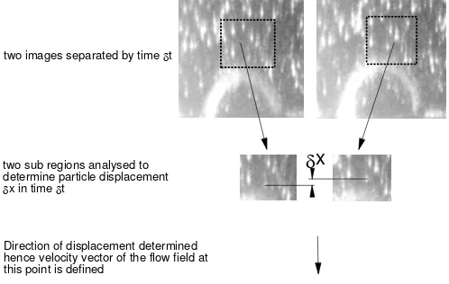
the flow field is referred to as autocorrelation. An alternative to autocorrelation is to analyse
two sequential images of the flow field; referred to as cross correlation. Cross correlation
produces a vector map of the flow field by analysing pairs of sequential images. In this
a particle, or group of particles, between exposures. If the time between exposures is known
then, combined with an analysis of the direction of the displacement, the velocity of the
particle and hence the flow in that region is known. This is shown on figure 2. Cross
correlation analysis is advantageous because it does not create any directional ambiguity
within the vectors calculated and is capable of measuring extremely low as well as a wide
range of velocities. For information on PIV in general the reader is recommended to consult
the paper by Gray [8].
δx
two images separated by time δt
two sub regions analysed to determine particle displacement
δx in time δt
[image:7.595.173.422.265.423.2]Direction of displacement determined hence velocity vector of the flow field at this point is defined
Figure 2: Cross correlation technique
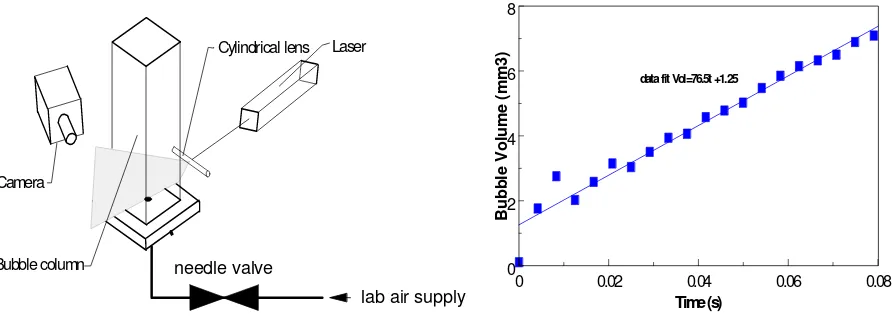
The particles in the flow were illuminated by a laser sheet produced by a 5W Spectra Physics
165 Argon Ion laser and cylindrical lens. Typically only 2.5W of laser power were required
for imaging purposes. The process of bubble formation was filmed by a Kodak Motioncorder
high speed digital video camera which had a capability of recording at frame rates up to 600
frames per second. Air flow was provided by the lab high pressure air supply regulated to a
lower pressure by a series of valves. The air was controlled by a needle valve situated
upstream of the orifice. The water column was 150mm square section and 300mm high
manufactured in glass with a 1 mm orifice at the base. A diagram of the experimental setup is
0 0.02 0.04 0.06 0.08 0
2 4 6 8
Time (s)
B
u
b
b
le
Vo
lu
m
e
(
m
m
3
)
[image:8.595.74.521.75.237.2]data fit Vol=76.5t +1.25
Figure 3 Experimental setup Figure 4 Bubble volume time history
Images were digitised by a Matrox frame grabber card in a 486DX266PC. The digitised
images were analysed by Optical Flow Systems VidPiv PIV analysis Software by cross
correlation on a Pentium P200 PC. To compensate for magnification within the optics a
reference grid was filmed and digitised to give the required scaling information. When the
acquired images had been digitised, pairs of images were analysed by cross correlation to
yield the vector field around the emerging bubble. The images discussed in this paper were
acquired at 240 frames per second. Timing is given from the first sign of bubble growth and
the image is the first of the pair used for cross correlation.
Furthermore, from the digital video images of the bubble during the growth process, the time
evolution of the bubble volume, surface area and centroid position were determined by
analysing the images in each frame. From the analysed images the volume flowrate was
determined for the test conditions as shown in Figure 4. It can be seen that the volume
flowrate is constant over the bubble growth period and was calculated to be 76.5 mm3/s.
Laser
Pump
Camera
Flow meter Settling chamber
Cylindrical lens
Bubble column
4. RESULTS
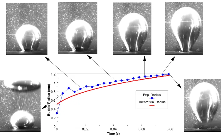
The mathematical model was used to predict the experimental test discussed above. A
comparison between the theoretical results and the experimental data are shown on Figs 5,6
and 7. Fig. 5 shows the experimentally measured bubble radius and the theoretically
calculated value in conjunction with the bubble images recorded during the test. It can be seen
that a reasonable prediction is achieved.
0 0.02 0.04 0.06 0.08 0
0.2 0.4 0.6 0.8 1 1.2
Time (s)
B
u
bb
le
Ra
di
us
(mm
)
[image:9.595.121.475.261.479.2]Exp. Radius Theoretical Radius
Figure 5 Comparison of experimental and predicted bubble radius
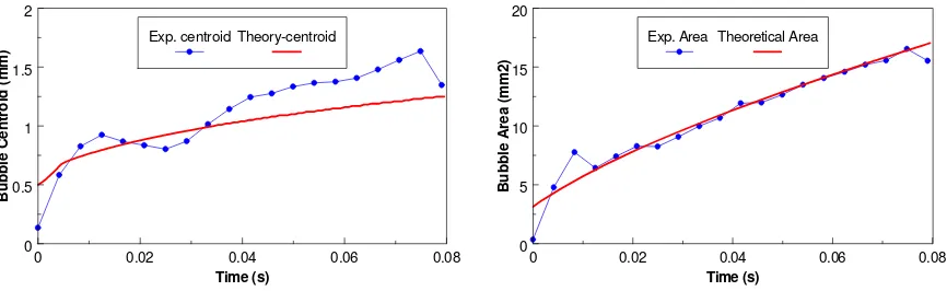
Figure 6 and 7 compare theoretical and experimentally derived bubble centroid position and
surface area. The centroid position, which represents the movement of the bubble is not very
well predicted by the theoretical model as can be seen in Fig 6. However, surprisingly the
0 0.02 0.04 0.06 0.08 0
5 10 15 20
Time (s)
Bubb
le Area (
m
m
2
)
[image:10.595.76.509.73.206.2]Exp. Area Theoretical Area
Fig. 6 Theoretical and exp. centroid position Fig. 7 Theoretical and exp. bubble area
While the reasonable predictions of bubble radius and surface area are reassuring, the
relatively poor prediction of the centroid position is of significance due to the fact that the
centroid position is indicative of the extent of bubble necking process and the effect of the
resultant forces acting on the bubble. To further clarify these deficiencies a number of the
predicted velocity fields have been compared with the PIV generated flow fields at 25, 50 and
75 msec during the bubble growth process and are shown on Figs 8a,8b and 8c The bubble
detachment from the orifice occurs at approximately 77 msecs.
0 0.02 0.04 0.06 0.08 0
0.5 1 1.5 2
Time (s)
Bubb
le Centroid (
m
m
Fig 8a Experimental and predicted vector field at 25 msecs
Fig 8b Experimental and predicted vector field at 50 msecs1
1
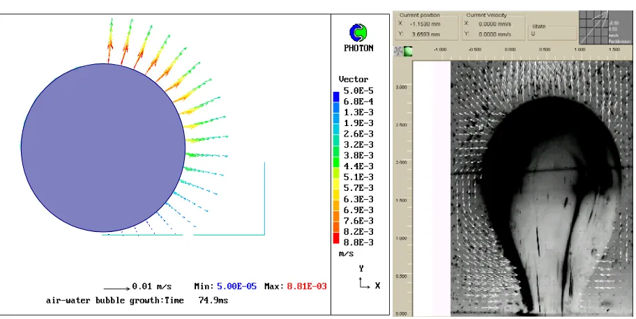
[image:11.595.72.528.435.664.2]Fig 8c Experimental and predicted vector field at 75 msecs
The PIV images of the predicted velocity field coupled with the photographic images allow
various features of the fluid flow to be ascertained. The velocity scaling for the predictions is
given on the right hand side of the image while the scaling for the PIV plot is given in the top
right hand corner. At present these images only allow a qualitative comparison when
compared with the mathematical model. However, certain important features of the flow
process surrounding the bubble can be discerned. In each of the figures the velocity field is
predicted to be dominated by radial flows that decay quickly as the radius increases. In the
PIV images much of the flow is dominated by a surrounding flow that has been generated by
the displacements of the previously detached bubbles. The extent of the influence of these
flows will depend on their magnitude compared with bubble surface values. For the test case
presented here where the growth rate is very small the effect of this influence will be
significant. It also noticeable that the PIV images indicate a circulatory flow at the lower part
of the bubble as it begins to neck. This is not predicted by the theoretical model to the same
extent and is likely to be indicative of poor predictions of the liquid inertia effects. To better
represent the circulatory nature of the flow with the current spherical model the translation of
the bubble centroid has to be better predicted since this movement will induce an up flow
beneath the bubble. Unfortunately, this movement will not be predicted without the correct
calculation of the inertia force. It would therefore appear that for the case studied the applied
modelling technique is not applicable.
5 CONCLUSIONS
A PIV technique has been developed to determine the velocity field around a bubble growing
mathematical model established from potential flow theoryand indicate potential problems in
the application in this type of modelling approach for air/water bubble growth problems.
6 NOMENCLATURE
a bubble acceleration
Ab bubble surface area
do orifice diameter
FB buoyancy force acting on bubble
Fσ surface tension force acting on bubble
FL liquid inertia force acting on bubble
Fe Excess internal pressure force due to surface tension
g gravitational acceleration
h centroid height from orifice plate
L height of bubble reference frame from orifice plate (see Fig. 1)
M Mass of bubble
ma orifice mass flowrate
P pressure
R bubble equivalent radius
u radial component of liquid velocity
uso steam velocity from orifice
Ub bubble velocity
v circumferential component of liquid velocity
Vb bubble volume
greek letters
ρl liquid density
φ_ liquid potential function
Δt time interval (between bubble images)
θ angle between top centre of bubble and position on circumference
α bubble contact angle at orifice
7 REFERENCES
[1] Tsuge H. Hydrodynamics of bubble formation from submerged orifices,
Encyclopaedia of Fluid Mechanics, (Edited by Cheremisinoff), Vol 3, Chapter 9, 1986
[2] R.T.Fox, A.T. McDonald, Introduction to Fluid Mechanics, Wiley (1985).
[3] L.M. Milne Thompson, Theoretical Hydrodynamics, Macmillan, (1965).
[4] A.S.Ramsey, A Treatise on Hydrodynamics, Part II:Hydrodynamics, G Bell & Sons
(1973).
[5] H.Lamb, Hydrodynamics, Dover Publications (1932).
[6] A.E. Wraith, T. Kakutani, The pressure beneath a growing bubble, Chem. Eng Sci.Vol.
29 (1974),p 1-12
[7] Arebi B, The formation and detachment of steam bubbles formed at submerged
orifices in sub-cooled water, PhD thesis, University of Strathclyde, Glasgow 1996
[8] Gray, C The evolution of particle image velocimetry, I.Mech.E Symposium on
Optical Methods and Data processing in Heat and Fluid Flow, City University,
London 1992