Computer vision to see people : a basis for enhanced human computer interaction

a basis for enhanced human computer interaction.

Gareth Loy

A thesis submitted for the degree of

Doctor of Philosophy

at the Australian National University

Robotics Systems Laboratory

Department of Systems Engineering

Research School of Information Sciences and Engineering

Australian National University

These doctoral studies were conducted under the supervision of Professor

Alexan-der Zelinsky. The work subn1itted in this thesis is a result of original research

carried out by myself, except where duly acknowledged, while enrolled as a PhD student in the Department of Systems Engineering at the Australian National

University. It has not been submitted for any other degree or award.

Firstly I would like to thank my supervisor Professor Alexander Zelinsky both for

his vision, insight and motivation , and the tremendous opportunities which he

provided to me during my PhD studies. Thankyou also to the other academics in

the department, in particular Professor Richard Hartley, Professor John Moore ,

and Dr David Austin whose guidance , support and insight have been invaluable.

To my fellow students in Systems Engineering with whom I 've shared the highs

and lows of post-graduate study, and who made the department such a great place

to work, Roland Goecke , Rochelle O 'Hagan, Dr Jo chen Heinzman , Dr J eremy

Thorne, Wayne Dunstan, Dr Tanya Conroy, Dr Louis Shue, Dr Llew Mason,

Leanne Matuszyk , Grant Grubb , Dr Simon Thompson , Dr Chris Gaskett, and

Matthew Smith, and special thanks to Luke Fletcher and Nicholas Apostollof

with whom I have had the pleasure to work with over the last year. Thankyou

also to the non-academic staff, James Ashton , Rosemary Shepard , Jenny Watkins,

Marita Rendina, and Karen Montefiore for all the assistance they have provided me over t he last few years .

During my PhD I was fortunate enough to spend several months at the University

of Western Australia in 2000, and The Humanoid Interaction Laboratory at AIST ,

Tsukuba, J apan in 2002. Thankyou to Dr Eunjung Holden and Professor Robyn

Owens for hosting me at the University of Western Australia and for the excit ing

t in1e we had working together, and thankyou to all my friends in P erth who

made my t ime there so enjoyable. Thankyou to Dr Gordon Cheng, Professor

Yasuo Kuniyoshi and Yoko Sato for hosting me in T sukub a and for making my stay such an enjoyable experience, and to my friends at Ninomiya House who made T sukub a a home away from home.

To the many other fabulous people who have touched my life over the few last

Damien Halliday, Emily Nicholson, Rosemary Driscoll, Shoko Okada, Catherine IVIoyle, Olivia Grey-Rodgers , Natalie Martino, Edwina Hopkins , Justine Lamond , Lars P etersson , Dirk Platzen and Annette Kimber, thankyou for your friendship , vitality and for the good times we shared. Special thanks to J essica Lye and Nina A1nini for so 1nany things , but especially for being truly outstanding friends.

Lastly, and most importantly I would like to thank my family, Rick, Winifred, Adele and more recently Scott, who have always been there for 1ne providing love, guidance, encouragement and support throughout n1y life.

Vision is the primary sense through which people perceive the world, and the im-portance of visual information during our interactions with people is well known.

Vision can also play a key role in our interaction with machines, and a machine that can see people is more able to interact with us in an informed manner. This

thesis describes work towards a computer vision system to enable a computer to

see people's faces, and hence provide a basis for more meaningful and natural

interaction between humans and computers.

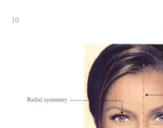
The human face possesses a number of visual qualities suitable for detecting faces

in images. Radial symmetry is particularly useful for detecting facial features.

We present new transform, the Fast Radial Symmetry Transform (FRST), that allows efficient computation of local radial symmetry in realtime. Both as a facial

feature detector and as a generic region of interest detector the FRST is seen to offer equal or superior performance to existing techniques at a comparatively low

computational cost.

However , no single cue can perform reliably in all situations. The key to an effi-cient and robust vision system for tracking faces or other targets is to intelligently

combine information frorn a number of different cues, whilst effectively

manag-ing the available computational resources. We develop a system that adaptively

allocates computational resources over multiple cues to robustly track a target in 3D.

After locating and tracking a face in an image sequence, we look at the problem of detecting facial features and verifying the presence of a face. We present an

automatic face registration system designed to automatically initialise features for

a head tracker. We also explore the problem of tracking the facial features. This involves tracking both rigid and deformable features to determine the 3D head pose, and describe the locations of facial features relative to the head. The 3D

features are then tracked relative to the head. A new fonn of te111plates was

introduced to facilitate tracking deformable features. These are used in two case

studies. The first is a monocular lip tracker , and the second is a stereo lip tracking

system that tracks the mouth shape in 3D.

The face localisation, feature detection and tracking solutions presented in this thesis could potentially be integrated to form an all-inclusive vision syste111

Thesis

Journal Publication

• Gareth Loy and Alexander Zelinsky. Fast Radial Symmetry for Detecting

Points of Interest. IEEE Trans on Pattern Analysis and Machine

Intelli-gence, Vol. 25, No 8, pp. 959-973, August 2003.

Conference Publications

• Gareth Loy and Alexander Zelinsky. A Fast Radial Symmetry Transform

for Detecting Points of Interest. Proc of European Conference on Computer

Vision (ECCV2002) . Copenhagen, May 2002.

• Gareth Loy, Luke Fletcher , Nicholas Apostoloff and Alexander Zelinsky. An Adaptive Fusion Architecture for Target Tracking. Proceedings of Fifth

In-ternational Conference on Face and Gesture Recognition (FGR 2002), Wash-ington DC , May 2002.

• Gareth Loy, Roland Goecke , Sebastian Rougeaux and Alexander Zelinsky.

Stereo 3D Lip Tracking. Proceedings of Sixth Int ernational Conj erence on

Control) Automation) Robotics and Computer Vision (ICARCV2000 ), Sin-gapore , December 2000.

• Eunjung Holden , Gareth Loy and Robyn Owens. Accommodating for 3D

head movement in visual lipreading. Proceedings of International

Confer-ence on Signal and Imag e P rocessing (SIP), pp. 166-171 , 2000.

Robotics and Automation ( A CRA2000 ), Melbourne Australia, August 2000 .

Provisional Patent

Statement of Originality

Acknowledgements

Abstract

Publications Resulting from this Thesis

1 Introduction

1.1 Principal Objectives

1.2 Key Contributions

1.3 Outline of Thesis .

1.4

1.3.1

1.3.2

1.3.3

1.3.4

1.3.5

Related vVork

A Fast Radial Symmetry Transform .

Face Localisation

Face Registration

Face Tracking

1.3.6 Conclusion .

Chapter Summary

2 Related Work

...

111

V

..

Vll

.

IX

1

3

5

5

6

6

6

7

7

8

8

2.1

2.2

2.3

2.4

2.5

Cues for P erson Tracking .

2.1.1

2.1.2

2.1.3

2.1.4

2.1.5

The H un1an Face

Skin Detection

Depth Maps

Motion . . .

Radial Sy1n1netry Operators

Face Localisation

Face Registration

Face Tracking ..

2.4.1

2.4.2

Tracking Rigid Facial Features .

Tracking Deformable Facial Features

Summary . . . .

3 Fast Radial Symmetry Detection

3.1 Definition of the Transform

3.2 Choosing the Parameters .

3.2.1 Set of Radii N

3.2.2

3.2.3

3.2.4

Gaussian Kernels A n

Radial-strictness Parameter a

N orn1alizing Factor kn

3.3 Refining the Transform . . . .

3.3.1 Ignoring Sn1all Gradients .

3.3.2 Dark & Bright Syn1metry

3.3.3 Choosing a Constant A n

3.4 A General Set of P arameters ..

3.5

3.6

Performance Evaluation . . . . .

3.5.1

3.5.2

Performance of the FRST

Comparison with Existing Transforms

Summary . . . .

4 Face Localisation

4.1

4.2

A Bayesian Approach to Target Localisation

4.1.1

4.1.2

Markov Localisation . . . .

IVIarkov Localisation vvith a Particle Filter

System Design . . . .

4.2.1

4.2.2

Part icle Filter

Cue Pro cessor

78 78

83

90

91

92

92

94 95

96

98

4.3

Localising and Tracking a Head in a Complex Environment .

102

4.4

4.5

4.3.1

4.3.2

4.3.3

4.3.4

In1plement ation

Prepro cessing .

Hypothesis Testing

Performance . . . .

Tracking Multiple . Targets

4.4.1

4.4.2

4.4.3

IVIultiple P article Filters

Experimental Setup .

Results .

Summary . . .

5 Face Registration

5.1

_{Automating the Detection of Features .}

5.2

5.3

5.4

5.5

Target Specification . . . .

Description of the System

5.3.1 5.3.2 5.3.3 5.3.4 5.3.5 5.3.6

Detecting Blink-like Motion

Extraction of Face Candidate Region

Enhancernent of Features .

Classifying Facial Features

Verify Face Topology . . .

Checking Similarity of Feature Pairs

Performance of Systen1

5.4.1

5.4.2

5.4.3

Implementation

Detection Perfonnance

Seeing Machines System

S un11nary . . . .

6 Face Tracking

6.1

6.2

Adaptable Ten1plates

IVIono cular Lip Tracking

6.2.1 IVIonocular 3D Head Tracker

6.2.2 :tv1outh Detection and Correction for P ose .

6.2 .3 Experimentation

6.2.4 Section Review

6.3 Stereo Lip Tracking ..

6.3.1 Stereo Vision System

6.3.2 Head Tracking.

6.3.3 Lip Tracking ..

6.3.4

6.3.5

Experimentation

Section Review

6.4

Summary . . . .

7 Conclusion

7.1 Summary

7.2 Achievements

7.2.1 Fast Detection of Radial Symmetry

180

185

186

187

187

189

189

7.2.2 An Adaptive Fusion Architecture for Target Tracking 189

7.2.3

7.2.4

Facial Feature Detection . . . .

3D Deformable Facial Feature Tracking .

7.3 Further Work . . . .

A Contents of CD-ROM

B Derivation of the Optical Flow Constraint Equation

190

190

191

193

1.1

1.2

2.1

2.2

2.3

2.4

2.5

2.6

Humans communicating . . . .

Enabling a computer to "see" a face .

Facial qualities suitable for detection by a computer

Average face . . . .

Constructing a skin colour model

Detecting skin . . . .

A stereo image pair and associated depth map

Pinhole camera model and stereo camera configurations .

2. 7 Laplacian of Gaussian

2.8 Difference of Gaussian

2.9 Example of a 3 x 3 neighbourhood centred on a point p

2

4

10

12

15

16

20

21

24

24

25

2.10 Result of Zabih and \iVoodfill 's rank transform with radius 1 25

2.11 Examples of different motion cues

2.12 Modelling fixation tendencies

27

31

2.13 Examples of Reisfeld et al. 's Generalised Symmetry Transform 31 2.14 Gradient orientation masks used by Lin and Lin . . .

2.15 Inverted annular template as used by Sela and Levine

2.16 The spoke filter template proposed by Minor and Sklansky

32

34

2.17 Example of Di Gesu and Valenti's Discrete Symmetry Transfonn . 35

2.18 Example of Kovesi 's sym1netry from phase .

2 .19 Evolution of particles over a single time-step

2.20 Cues operating in Triesh and von der Malsburg's system

2.21 Triesh and von der Malsburg's syste1n in operation

2.22 Face registration

2.23 The kernel used by Yow and Cipolla (1997) .

2.24 3D pose of a head and head reference frame

2.25 3D reconstruction from stereo images . . .

36 38 41 42 44 45 49 51

2.26 A right angle triangle fro1n the ith camera in Figure 2.25 52

2.27 Example of Matsumoto and Zelinsky's head tracking system 56

2.28 The appearance of a subject's mouth can vary greatly .

2.29 Reveret and Benoit's lip 1nodel

3.1 Steps involved in co1nputing the FRST

3. 2 The locations of affected pixels

3.3 3.4 3.5 3.6 3.7 3. 3.9

Effect of varying radii at which the FRST is computed

The contribution of a single gradient element .

Effect of varying a . . . .

Some example i1nages from the test set

IVIean and standard deviation of the maxi1num of On

The effect of different values of f3 on S .

Examples of dark and bright sy1n1netries

3.10 256 x _{256 lena in1age . . . .}

3.11 Results of applying the FRST to the 256 x 256 lena i1nage

3 .12 The FRST applied to face and other images .

3.13 The FRST being calculated online in realtime

3.14 Comparison of performance on an outdoor image

3.15 Comparison of performance on the standard lena image

81

82

87

88

3.16 Comparison of performance on an image of a face in half shadow . 89

4.1 4.2 4.3 4.4 4.5 4.6 4.7 4.8 4.9

The four steps of the particle filter.

System architecture.

Particle filter tracking a head in ( x , y, z, 0) state space . Example of particle population evolving over time

Sensing process . . . .

Preprocessing a colour stereo image pair

Generic head target and associated search regions

Several frames in tracking sequence

Frame in tracking sequence . . . . .

4.10 Cue utility and associated processing delay

4.11 Two particle filters tracking separate targets

4.12 Preprocessing results from single camera

4.13 Some snapshots of the system running

4.14 Some snapshots of the system running

4.15 Some snapshots of the system running

5.1

5.2

5.3

Average face and facial dirnensions . . . .

Average face showing placement of the mouth and nose

Structure of face-finding algorithm. . . . . .

5.4 Detection of blink-like motion. 128

5.5 Process for extracting potential face region fro1n image buffer. 130

5.6

5.7

5.8

5.9

Face region defined in terms of the interpupillary distance

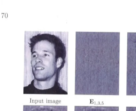
Process for enhancing features in face region. . . .

Images associated with the enhancement process.

Regions Si used by Li for enhancing facial features 5.10 Procedure for locating facial features. . . .

131

132

133

134

135

5.11 Process for locating feature rows using integral projection . 136

5.12 Process for locating feature columns within each feature row 136

5.13 Closeup view of a human eye .

5.14 Process for locating eyes . .. .

138

138

5 .15 Region used by local comparison operator to highlight sclera 139

5.16 Process for locating mouth corner. . . 140

5.17 Lo cal comparison operator regions for enhancing the mouth 141

5.18 Lo cating nostrils

5.19 Eli1nination of non-plausible nostril pairs

5.20 Eyebrow detection. . . . . .

142

143

144

5.21 The similarity of symmetrically opposite features is verified. 146

5.22 Snapshots of a sequence . . . .. .

5.23 Results of the syste1n on a range of subj ects

5.24 Results from the Seeing Machines implementation

6.1

6.2

6.3

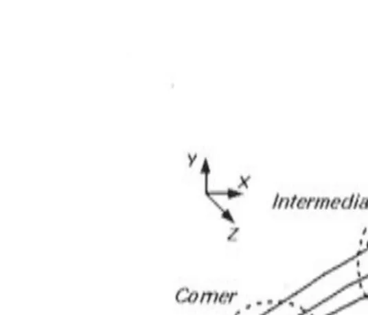
Te1nplate matching . . . .

Ten1plate matching a defonnable feature using

3D pose of a head and head reference frame .

6.4

6.5

The process t he head t r acker steps t hrough each fr am e.

Pinhole can1er a rnodel. . . .

158

161

6.6

Face in1age sho,;ving proj ected feature lo cations and search regions

162

6.7

6.8

6.9

Searching procedur e using init ial sp arse search . . . .

Search lines for locating t he t op and bottorn n1out h edges .

Projection of n1out h points fron1 in1age plane t o face plane.

6.10

Son1e sn ap shots of t he systen1 in oper ation . . .

6

.11

Results of t he head and 1nou t h t r acking systen1

6. 12

Overvie,~r of t he systen1.

6. 13

The stereo ca1ner a arr angem ent .

6.1 4

Pri1nary t r acking p oints

6.1 5

Lip t r acking syste1n.

6. 16

Search lines placen1ent

6.1 7

Conto ur t r acking te1n plates

6.18

The syste1n in op eration ..

6. 19 3D

error in pri1nary featur e locations .

6.20

Abso lute error in x-direction in prin1ary featur e locations ..

6.21

Abso lute error in y-direction in prin1ary featur e locations . .

6.22

Absolute error in z-direction in pri1nary featur e locations ..

163

167

168

170

171

173

174

175

175

178

179

181

182

183

183

2.1

2.2

3.1

3.2

3.3

3.4

Face Dimensions of British Adults . . . .

Head Dimensions Bounding Populations

P ar ameter Settings used for Experimentation .

P arameter Settings used for Exp eriment ation .

Estimated Computation Required for Different Transforms

Computational Order of Different Tr ansforms . . . .

11

11

69

78

84

86

5.1 Estimated Computations per Frame . . . 147

6.1

6.2

6.3

Estimated Computations p er Fran1e . . . .

I'v1ean absolute error in primary t r acking points.

Estimated Co1nputations per Frame . . . .

169

182

Introduction

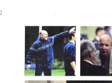
Interpersonal communication is a central part of people 's lives. The purposes of communicating with other p eople are many and varied . We commonly com-municate who we are, what we are doing, or how we are feeling, and instruct others how to do things, or wh at we would like them to do . P eople communicate effortl essly using language , tone of voice, gestures , posture and facial expressions. A significant proportion of this communication is non-verbal. Figure 1.1 shows people communicating in different circumstan ces - just by observing t he people in these pict ures we can tell quite a lot about their situations, and begin to guess what it is they are communicating.

There is some debate amongst experts as to exact ly how much interpersonal communication is non-verbal. Birdwhistell (1970) estimates 65 percent of the in-formation transferr ed in a normal two person conversation is non-verb al, whereas

1ehr abian (1972) postulates it o be as high as 93 p ercent . The precise value is of lit le consequence , t he point is t hat non-verbal - as well as verbal - commu-nication pla s a crucial role in t he interaction between people.

Compared to the way people interac with each other our interaction with com-puter ( and robot ) is much more restricted . Traditionally people have interacted with computer using a keyboard and mouse or other pointing device, and whilst the e are -ell uited for mo t standard computer tasks it limit computers to these ( tand ard'' ta ks. B:; tandard ta ks we mean ta ks that computer are

tradition-ally _{considered a being good a , uch a word proces ing, databa e management ,}

[image:26.1177.150.598.114.448.2]

Figure 1.1: Humans communicating.

Enhancing the interaction between humans and computers offers many new pos-sibilities. Ideally we would like to be able to interact with a computer in the same way we do with another person. This would open the door to many new and useful applications. Potential tasks could include:

• entertainment, interfaces for games, facial animation,

• in1proved teleconferencing ,

• monitoring human performance,

• classroom teaching,

• caring for the elderly, or the disabled,

• smart cars , sn1art devices,

• smart security surveillance, and

• n1aking n1anual or automated tasks easier .

1.1

Principal Objectives

The goal of this research is to work towards a computer vision system that enables a computer to see people's faces, and hence provide a basis for more meaningful and natural interaction between humans and computers. What do we mean when we say we want a computer to be able to "see" faces? We want the computer to be able to locate and track humans in image sequences , preferably in real-time, and with robustness to different people's appearances and the operational environment.

There are a number of aspects to this problem. Firstly it is necessary to know where a person is in a scene, in particular the location of their head. Once the approximate location of the head is known the facial features can be detected, and once these features have been found they can be used to track the pose of the head and the relative motion of deformable features such as the mouth and eyebrows. This thesis aims to present solutions to these human tracking issues that could potentially form an all-inclusive vision system to allow a computer or robot to see a person 's face.

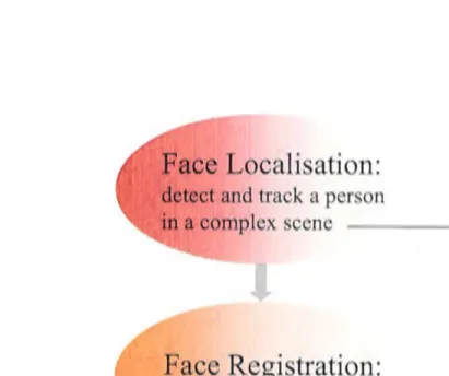
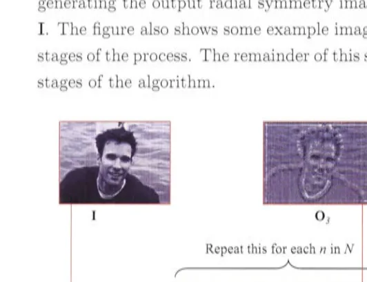
Figure 1.2 shows how the problem of enabling a computer to see faces can be broken down into face localisation, face registration , and face tracking. It also shows how these different stages of the process relate directly to human com-puter interaction applications such as human motion capture, face recognition , lip reading and expression recognition.

The first , and perhaps the most challenging problem to be dealt with, is face localisation. Consider the situation where a person is moving around a room, the lighting conditions are variable, sometimes there are objects occluding the person 's face , there may even be more than one subject to be tracked, and the camera is not assumed to be stationary. The face localisation module must ro-bustly locate the approximate location of the face and track it. It would be feasible to extend this module to locate other parts of the body in addition to the face , and move onto full or partial human motion capture, or even gesture recognition. However , for the purpose of this work we are primarily interested in locating the face.

Face Localisation:

detect and track a person

in a complex scene

Face Registration:

Example applications

Human motion capture

detect facial features - - - Face recognition

Face Tracking:

Track head pose - - - Gaze point estimation Track facial features _{Lip reading,}

[image:28.1177.197.609.182.526.2]

expression recognition

Figure 1.2: Overview of enabling a computer to "see" a face, and some typical applications associated with the different stages.

is desired to automatically recognise t he face from a set of known faces , then the facial feature locations fron1 the face registration module can be lised to normalise t he app earance of the face in preparation for the application of a face recognition algorithm.

Once facial features have been detected it is possible to track the pose of the head and track t he relative lo cations of deformable facial features. This essentially captures all the inforn1ation the fac e has to offer without determining a dense 3D n1odel of t he subject . From here it is feasible to perform lip tracking; automate a facial avatar, or attempt expression recognition.

This thesis will focus exclusively on capturing visual information describing the face , thus enabling a computer to "see;; a face. Face localisation , registration, and tracking are each considered in t urn and examples of implementations of each of these are presented. Fast and efficient visual cues are also considered in detail; and these cues are app lied to the variou detection and t racking tasks required.

Consequently, the methods developed in this thesis have a strong emphasis on

speed and efficiency. All algorithms were initially implemented in Matlab,

how-ever, some realtime implementations have been ma~e using C++. Furthermore, while the Matlab implementations typically run quite slowly, the algorithms are

efficient enough to run in realtime in C/C++.

1.2

Key Contributions

• Fast detection of radial sym1netry - a valuable cue for detecting eyes and

other radially symmetric features in images.

• A system to adaptively allocate computational resources and fuse cues for

robust person tracking.

• Face detection algorithm for initialisation of a head tracking system.

• A monocular and a stereo 3D lip tracking system, both operating in

conjunc-tion with 3D head trackers to allow the subject's head freedom of movement whilst tracking.

1.3

Outline of Thesis

Chapter 2 discusses the application of computer vision for locating and track-ing people, in particular the face , and reviews previous research in this area. In

Chapter 3 a novel i1nage based transform is presented that allows efficient

com-putation of radial symmetry in realtime; this transform is a powerful visual cue

for face detection and is used in the systems described in the Chapters 4 and 5.

Chapter 4 presents a vision system that adaptively allocates computational

re-sources over n1ultiple cues to robustly track targets in 3D. In Chapter 5 a system is described that performs automatic detection of facial features for the process of

face and gaze tracking. Chapter 6 explores the problem of tracking the face and deformable facial features such as the lips. Finally, Chapter 7 closes the thesis with a summary of the key findings and suggestions for further research.

1.3.1

Related Work

Chapter 2 reviews related work in the field. We discuss the physical qualities

governing facial app earance, and consider visual cues suitable for detecting faces in images. We then move on to look at previous research relevant to lo cating a face

( or other specified target) in a cluttered and dynamically changing environment,

placing particular emphasis on the need to fus e multiple visual cues in order to obtain a robust esti1nate. Next we review previous work on face registration,

that is , verification that a face is present and detennining the location of facial

features. Then we look at face tracking, both tracking of the head pose and

tracking defonnable facial features such as the mouth. Finally the chapter closes

with a su1nn1ary of the key points.

1.3.2

A Fast Radial Symmetry Transform

Chapter 3 presents a new i1nage transform that utilizes lo cal radial sy1nmetry

to highlight points of interest within a scene. Its low computational complexity

and fast run-ti1nes make this method well suited for realtime vision applications .

The perforn1ance of the transform is demonstrated on a variety of images and

con1pared with leading techniques fro1n t he literat ure. Both as a facial feature

detector and as a generic region of interest detector t he nevi transform is seen to

offer equal or superior p erformance to contemporary techniques at a relatively low

computational cost . A real time implement ation of the t ransform is also presented

den1onstrating the effectiveness of the transfonn for highlighting p eoples eyes in real time .

1.3.3

Face Localisation

Chapter 4 considers the problen1 of fac e localisation in a co1nplex, d) namic en-vironn1ent. A vision syste1n is presented that adaptively allocates computational

resources over multiple cues to robustly track a target in 3D. The system uses a

particle filter to maintain n1ultiple hypotheses of the target location. Bayesian probability theory provides the framework for sensor fusion , and resource

schedul-ing is used to intelligentl allocate the limited computational resources available across the suite of cues. The sy te1n is shov\ n to track a person in 3D space

how the system can be extended to track multiple targets , using multiple particle

filters, and inhibition of returns to prevent different filters from locking onto the

same target.

1.3.4

Face Registration

Chapter 5 examines the problem of face registration, that is, automatically de-tecting facial features and confirming the presence of a face in an image. A face registration system is presented that is designed to perform automatic detection

of facial features for the purpose of face and gaze tracking, and hence provide the capability of face tracking without the requirement of a user specification or

calibration stage. Motion information is used to detect blinks, indicating

possi-ble eye locations and an associated face candidate. Facial features ( eyes, mouth

corners, nostrils and eyebrows) are located and the face candidate is verified by

examining the topology of these features.

1.3.5

Face Tracking

Chapter 6 explores the problem of tracking the face and deformable facial features

such as the lips. In order to effectively track deformable facial features relative to

an unconstrained head it is also necessary to track the head pose. In this chapter

two case studies are presented , the first is a monocular lip tracker, and the second

is a stereo lip tracking system that tracks the mouth shape in 3D.

Tracking the lips has a broad scope of applications across the field of

human-con1puter interaction, including animation, expression recognition , and

audiovi-sual speech processing. As people talk, their heads naturally move about as they

gesture and follow conversation cues.

It

is necessary for a lip tracking system to be robust with respect to this behaviour ; to be able to detect , monitor and

account for rnovement of a speaker's head.

The mouth is a 3D feature which deforms 1n all spatial dimensions. In order to fully describe the mouth shape it is necessary to track it in 3D. Providing

1.3.6

Conclusion

Chapter 7 closes the thesis with a summary of the key findings and achieven1ents ,

and suggestions for further research.

1.4

Chapter Summary

This chapter has introduced and motivated the research reported in this thesis. We have discussed the importance of visual information in both interpersonal

interaction between people and hun1an-computer interaction, and stressed the

point that a computer that can see people is significantly closer to a co1nputer

that we can interact with like we do with other human beings. The reader was

then introduced to the problem of enabling a computer to see a person , and given

a breakdown of a number of key elements of this problem. Finally we presented

an overview of the research in this thesis, showing how it contributes towards

Related Work

In the first chapter we discussed how the problem of enabling a computer to "see" a face can been broken down into face localisation, face registration and face tracking. This chapter reviews previous research in each of these three areas. The anatomy of the human face is also discussed along with visual cues suitable for detecting faces in images.

The first section of this chapter opens with a discussion of the physical qualities governing the appearance of a face , and reviews visual cues suitable for detecting faces in images. The following section reviews previous research relevant to lo-cating a face ( or other specified target) in a cluttered and dynamically changing environment ; particular emphasis is placed on the need to fuse multiple visual cues in order to obtain a robust estimate. The third section reviews previous work on face registration, that is , verification that a face is present and determining the location of facial features. In the fourth section a brief background of face tracking is presented , this involves both tracking of the head pose and tracking deformable facial features such as the mouth. The chapter closes with a summary of the key points.

2.1

Cues for Person Tracking

2.1.1

The Human Face

Constrainedsetof - -- - - . face dimensions

Facial features: specific arrangement, ' : r 4 '

--~-typically darker than surrounding skin

Figure 2.1: Facial qualities suitable for detection by a computer.

hearing, taste and smell - _{are perceived by organs within the facial region} and fron1 another person's face we can sense hov.r they are feeling , ·where their attention is focussed: and even make an educated guess as to v. hether t hey are lying or Tuithholding infonnation . With 7,000 discrete facial expressions (Bates and Cleese. 2001 ) at our disposal t he face is rich with information, so it is not

urpri ing that the face is our prin1ary fo cus when we interact with others. Indeed uch interactions are often referred to as face -to-face encounter .

\\ l1at qualitie does the face ha, e that n1ake it look like a face , and -;-, hich of

the equalities can be used by con1puter vision to allow us to automatically locate face in in1age ? _{Figure 2.1 ho"\"\-s a frontal view of a face \Vi th a number of vi ual}

attribute indicated that are suitable for detection by a computer \1i ion ystem.

[image:34.1177.119.644.94.508.2]

Table 2.1.

Table 2 1 · Face Dimensions of Brit ish Adults ..

Dimension Men Women

Mean (mm) SD (mm) Mean (mm) SD (mm)

Head length 195 8 180 7

Head breadth 155 6 145 6

Maximum diameter of chin 255 8 235 7

Chin to top of head 225 11 220 11

Ear to top of head 125 6 125 8

Ear to back of head 100 7 100 9

Bitragion breadth 135 6 130 5

Eye to top of head 115 7 115 9

Eye to back of head 170 8 160 10

Interpupillary breadth 60 4 60 4

ose to top of head 150 10 145 12

Nose to back of head 220 9 205 10

Mouth to top of head 180 9 170 11

Lip length _{50 5 45 4}

We desire our system to be able to detect anyone, regardless of race, sex, age or stature. With this in mind we look at head sizes from different populations, in an attempt to determine a range of head sizes within which every person will lie. Examining anthropometric data from Pheasant (1986) for males and females from orth American, British, French, Swiss, German, Swedish, Polish, Japanese, Hong Kong Chinese and Indian populations we find the American male has the largest adult head size, and the smallest is that of Indian women. Thus we have a range within which we expect adult head sizes to fall. Including children in the search space will lead to a broader range of acceptable head sizes , however , if we restrict ourselves to only searching for children above five years old this only slightly extends the acceptable range of head sizes. Table 2.2 presents the head dimension of these bounding populations. Note that only British data was considered for children.

Table 2.2: Head Dimensions Bounding Populations

Population _{Head length Head bread th}

Mean SD Mean SD

Newborn infants (British) 120 4 _{95 3}

5 year old girls (British) 165 8 130 5 Smallest adult (Indian female) 170 7 135 5

Largest adult (American male) 195 8 155 6

Figure 2.2: Average face.

t he facial features aligned. Average faces have been used previously in computer vision to search for faces in images ( Cai and Goshtasby; 1999) i and in studies

of human facial beauty (Grammer and Thornhill ; 1994) . However; t hese average faces have typically been constructed from a n1odest number of faces ( Cai and Goshtasby used 16 ; and Grammer and Thornhill (1994) constructed male and female average faces using 44 and 52 subjects respectively). \i\ e· have constructed an a-.-erage face from 224 images of faces of men and women of different races obtained from the internet. Each image was rotated so t he eyes were horizontal ; and warped so the interpupillary distance and the distance from the mouth to the eyes \\-ere the same acros all images. The ratio of the interpupillary distance to n1outh to eye di tance \\-a determined by averaging the male and female pop-ulation in Table 2 .1 (gi\-ing a ratio of 1: 1) . _{The resulting average face is shown}

in Figure 2. 2. The a\-erage face provide a useful reference for designing cue to detect face and facial feature in image .

face-like arrangements is difficult to do efficiently and robustly, however , these facial

qualities are useful to check when it comes to verifying whether or not a detected

target is a face.

The remainder of this section reviews previous research 1n this area, covering

skin detection, depth map estimation, motion detection , and radial symmetry

detection.

2.1.2

Skin Detection

Detecting skin regions 1s a first step in the majority of recent face detection

methods. The key quality that differentiates skin from non-skin regions in

im-ages is colour. Colour has been successfully used to identify regions of human

skin in i1nages in numerous applications. Interestingly, human skin colour varies

little between different races. The primary variation is in its intensity, that is

proportional to the amount of melanin in the skin.

Swain and Ballard (1991) demonstrated that the intersection of colour histograms

in colour space could be used to reliably identify coloured objects. However , this

technique was sensitive to colour intensity and thus the ambient light source.

Several years later Hunke (1994), Hunke and Waibel (1994) and Schiele and

Waibel (1995) developed a skin colour detector which was invariant with respect

to intensity. They modelled colour in a two dimensional chrominance space1

obtained by normalising the RGB colour space with respect to intensity (see

equations 2.1 and 2.2). Since this time a plethora of different skin colour detection

schernes have been reported in the literature.

The general approach of skin colour segmentation schemes is summarised as fol-lows.

Initially a skin colour model is built off-line, this involves:

• Sample colour images containing only skin colour are passed to the system (these are typically in RGB format), Figure 2.3(a).

• The colour value of every pixel is mapped to a two dimensional chrominance

space (some schemes map to a colour space with three dimensions , but these

1

A chrominance space is a two dimensional space generated by removing the intensity

are in the minority) to form a skin colour histogr an1. Figure 2.3(b).

• A model is selected describing the distribution of skin colour pixels 111

chrominance space. Figure 2.3(c).

Testing images for skin colour is done on a pixel-by-pixel basis as shown in

Fig-ure 2.4:

• The colour infonnation is converted to the appropriate chrominance space.

• The skin-likeness of each pixel is determined by the value of the skin colour

distribution function corresponding to the pixel 's location in chron1inance

space.

A threshold is generally applied to the output to produce a binary image of

skin-coloured regions, however , pixels can be left as grey-levels giving a continuous measure of how "skin-like" they appear.

The main differences between different skin colour detection schemes are the

chro1ninance space chosen , and the distribution used to model the skin in chro1ni-nance space.

The effectiveness of a skin detection algorithm depends on tpe appropriateness

of the chrominance space in which the skin chroma is modelled. It is desirable

to use a space in which the skin chroma distribution can be accurately modelled

and segmented from non-skin chroma. Just about every colour space ( or corre-sponding chro1ninance space) has been used for skin colour detection , examples

include RGB (Satoh et al., 1997) , nonnalised rg (Hunke, 1994 ; Ku1nar and P og-gio, 2000) , HSY (Sobottka and Pitas , 1996a) , CIE (Co1nmission Internationale

/

de L'Eclairage) XYZ (Wu et al., 1999), CIE LUY (Yang and Ahuja, 1998) , and CIE Lab (Cai and Goshtasby, 1999).

Two recent studies have compared the performance of different colour spaces

for hu1nan skin detection (Terrillon and Akamatsu, 1999; Zarit et al., 1999) , whilst these studies fail to agree on an optimal colour space , results from both

studies support the HS chro1ninance space as exhibiting the smallest overlap

between skin and non-skin distribution. Terrillon and Akamatsu (1999) exa1nine

the comparative performance of nine different colour spaces applied to detecting

( a)

a

b

-JO O JO 20 30 40

(b)

a

b

-JO O JO 20 30 40

(c)

Figure 2.3: Constructing a skin colour model. (a) Image of multiple skin

samples. (b) Plot of chrominance values in ab _{chrominance space, from Cai}

and Goshtasby (1999). (c) Example skin chrominance model in ab space, from

I

pixel l(p)

(a)

b

-10 0 10 20 30 40

b .

l

(b)

(c)

skin colour distribution model. They test normalised rg, CIE-xy, TS, CIE-DSH, HSV, YIQ, YES, CIE LUV and CIE LAB and conclude that their own TS chroma

space (Terrillon et al., 1998) designed especially for _this purpose shows the best results, followed by the normalised rg space. Zarit et al. (1999) compare the performance of CIE LAB, Fleck HS, HSV, normalised rg and YCrCb with two different skin colour modeling schemes and conclude that HSV and Fleck HS

provide superior performance.

From these studies on classification performance, normalised rg, HS and TS chrominance spaces appear are the most effective for skin segmentation. However,

classification performance is not the only factor that needs to be taken into

con-sideration. The computational load of converting to different chrominance spaces

is also an important factor when choosing a chrominance space for realtime skin

detection.

Video cameras generally deliver raw colour image information to a computer in

YUV format, where Y is a full resolution luminance channel and U and V are

chrominance channels, with one value for every two pixels. These are converted

to standard RG B format for storing in memory and displaying on the screen, and

as a result the majority of colour conversions consider RGB as the base colour

type. The normalised rg chroma, for instance, are calculated from the RGB colour values using,

R

T =

-R+G+B

(2.1)

G

g=

R+G+B

(2.2)

The TSL space which leads · to the TS chroma is defined as (Terrillon and

Aka-matsu, 1999)

S=3!f-T=

L

=

0.299R

+

0.587G

+

0.114B

where r'

=

r -

½

and g'

=

g-

½,

and r and g are defined by Equations 2.1 and 2.2. However, there is no reason why the raw UV chrominance information cannot

be used for skin segmentation. The YUV colour format provides us with a

pre-calculated chrominance image that requires no additional con1putation to

gener-ate.

The second key element in a skin-colour extractor is the model used to represent

the skin colour distribution in chrominance space. Such models range from

prin1-itive rectangular regions achieved by thresholding of chrominance values

(Sobot-tka and Pitas, 1996b) to e1npirical histogram look-up tables (Hunke and Waib el,

1994) and sophisticated probabilistic and statistical models (Yang et al., 2000;

Wu et al., 1999).

Some researchers (Yang and Waibel , 1996; Yang and Ahuja, 1998) have

hypoth-esised that all skin colour - regardless of race - can be satisfactorily modelled by

a single multivariate Gaussian distribution. It is true that skin values in

chro1ni-nance space deviate little due to race , however, so1ne subjects do exhibit slightly

different skin chrominance distributions independently of race (Omara, 2000).

This observation has led to a number of more complex skin models, exa1nples

in-clude multiple Gaussian distributions ( Omara, 2000 ), fuzz y modelling techniques

(Wu et al., 1999) and neural network based designs (Chen and Chiang, 1997). Cai and Goshtasby (1999) proposed a simple numerical technique for building

a skin colour look-up table in chron1inance space. The result is effectively a numerical approximation of a complex multi-Gaussian model , and is obtained

by convolving the chroma histogra1n with a Gaussian to make a "skin cloud" in

chro1na space. This approach is very attractive as it offers a diverse and accurate

1nodel with the speed of an empirical lookup table. The drawback is that it

-is difficult to adapt the skin 1nodel to changing lighting conditions, since it -is

not represented as a fonnal statistical distribution function. This sensitivity to lighting conditions is the 1nain shortcon1ing of skin colour detection sche1nes, and

while the use of intensity invariant chroma spaces has reduced this sensitivity, it is still a problem.

So1ne researchers have considered adapting skin colour models to varying lighting

1nodify the parameters of their Gaussian n1odel to adapt to changes in lighting

during operation. Raha et al. (1998) used Gaussian mixture 1nodels to detect skin colour, hair, and clothing and presented a techniqu: for dynamically updating

these models to account for changing lighting conditions. Sigal and Sclaroff (2000)

use a Hidden Markov Model to evolve a skin colour distribution model in HSV

colour space , and claim their system reliably extracts skin under widely varying

lighting conditions - including multiple sources of coloured light.

An alternative approach is to simply build the original chrominance histogram

using samples from all lighting conditions under which the syste1n is intended

to operate. These conditions cannot be too diverse or the histogram could

po-tentially contain all possible colours, however , for a constrained set of lighting conditions this is a feasible approach.

Vve base our approach to skin detection on that of Cai and Goshtasby (1999)

·which offers a fast , efficient and sin1ple method that delivers a high level of

per-formance. Hov\rever , vve augment the method by building a three-dimensional

skin colour histogram to better discriminate across varying lighting conditions.

Also , rather than using CIE Lab colour space we use YUV since these

chan-nels are available directly from our cameras and saves performing the additional non-linear conversion to CIE Lab space.

2.1.3

Depth Maps

Stereo in1ages have long been used for calculating depth in computer vision

ap-plications (Jarvis , 1983). There are other means of esti1nating depth that do not

require stereo , such as using a single camera and varying the focus , estimating

structure fro1n motion , or even shape from shading. However , stereo is by far the

most popular and robust method of estimating depth in the near field ; indeed

stereo is a strong cue for human depth perception for distances up to 10 meters. Figure 2.5 shov\rs an example of a pair of stereo images and a depth map generated

fron1 these images. The generation of such depth maps is discussed belovv.

Stereo imaging is best illustrated using the pinhole camera model to represent

t he cameras in\ olved. This model is shovvn in Figure 2.6 ( a) and demonstrates how each pixel in the i1nage corresponds to a ray in 3D space - so an object

visible at a particular image point could lie anywhere on the ray through t hat

(a) (b)

(c)

Figure 2.5: A stereo image pair and associated depth map, courtesy of Luke Fletcher. ( a) Left image. (b) Right image . ( c) Depth map with lighter values indicating shallower depths.

where two cameras are looking at same point. An object observed by camera

A lies on a ray that appears as a line in camera B. This is called an epipolar

line , and is dependent entirely on the epipolar geornetry of the cameras, that

is , the location and orientation of the carneras with respect to each other , and

the internal parameters of the ca1neras. The epipolar geo1netry is independent

of the objects in front of the camera, so regardless what images are observed, a

-particular image location will always correspond to the same epipolar line in the

other ca1nera view. All epipolar lines radiate out from a fixed image point called

the epipole , which is the image of the centre of the other camera, as shown in the

figure.

When vve are computing depth maps we are essentially just computing a series of

point correspondences between the two images. So given a point in image A we

y

X

Camera A

epipole e

X

Camera A

image point

image plane

(a)

baseline

(b)

epipole e'

Camera B

(c)

y '

z'

image B. A straightforward expression for determining the epipolar lines can be determined by calculating the epipolar geometry and determining the fundam

en-tal matrix (Hartley and Zisserman, 2000). However, this is not necessary if we

set up the cameras in an aligned configuration as shown in Figure 2. 6 ( c). This requires both cameras to share the same X-axis ( or alternatively Y-axis) , have parallel optical axes , and coplanar image planes. calculating a stereo depth map. In this configuration an image point at height y in one image will correspond to a horizontal epipolar line at height y in the other image . Since the cameras

are directly side-by-side the epipoles are located at infinity, hence the parallel epipolar lines.

The depth of an object observed in two stereo images fron1 calibrated aligned cameras can be determined from the disparity2 _{between the object 's location in}

the two images. The problem of determining the 3D depth map, such as the one shown in Figure 2.5(c), (or equivalently the disparity values) from a pair of stereo images comes down to finding the corresponding locations of points in the both images , this is referred to as stereo matching.

When constructing dense depth maps area-based matching techniques are used to solve the stereo matching problem. A number of different area-based techniques are available (Aschwanden and Guggenbuhl , 1993). Denoting the template win-dow as Ii , the candidate window as 12 , the mean pixel values of these windows as

I1 and I 2 resp ectively, and summation over the window as L (u ,,v)E W , these are:

• Sum of Absolute Differences ,

L

II1(u, v) - I2(x

+

u, y

+

v)I

(u ,v)E W

• Zero mean Sum of Absolute Differences ,

L

l(I1(u, v) - 11) - (I2_(x

+

u, y

+

v) - I 2)I

(u ,v) El¥

• Sum of Squared Differences,

L

(I1(u, v) - _I2(x

+

u, y

+

v)) 2

(u ,v) EW

2 _Disparity

• Zero mean Sum of Squared Differences,

L

((I1(u, v) -

1\) -

(I2(x

+

u, y

+

v) -

1

2 ))2

(u ,v) EW

• Normalised Cross Correlation,

I: (u ,v) EW I1(u, v) · I2(x

+

u, y

+

v)

• Zero mean Normalised Cross Correlation,

Regardless of ·which 1nethod is used , generating a dense depth map across an entire in1age is a computationally expensive procedure , as each in1age location n1ust be matched ·v.rith every other location on t he corresponding epip olar line in the second image. In t he late 1990 's Konolige (1997) and Kanade et al. (1996) both den1onstrated systems able to generate dense depth n1aps in real t ime, however, these systems relied on specialised hardware. In 2000 Kagan1i et al. presented a method for efficiently generating dense depth n1aps in realtin1e v\rithout requiring specialised hard·ware. This was achieved by using four key techniques: recursive nonnalised cross correlation , cache optimisation, online consistency checking, and use of the Intel 1vIMX/ SSE(R) instruction set.

Preprocessing of i1nages before perforn1ing stereo matching can increase the ef-fectiveness of the 1natching process. Preprocessing typically involves filtering in1ages to increase local contrast , and is particularly advantageous for 1natching areas with lov\r texture. Standard linear filtering approaches used are Laplacian of Gaussian (LoG ), or Difference of Gaussian , both of which increases local contrast in the image. The LoG is the sum of the Gaussian 's second derivatives. Fig-ure 2.7 shows a Gaussian , the first derivatives in the x and y directions and the LoG , V2G. _{Applying a LoG across an in1age involves convolving the LoG kernel}

V2_{G across the in1age. Unfortunately this kernel is non-separable, herefore the}

convolution cannot be split into two one-dimensional convolutions , and is of order O(K l\ 2) for an l\ x l\ kernel across an in1age y\rit h K pixels.

a¾

_ax

a%

8y

y

Figure 2.7: Laplacian of Gaussian. From top to bottom: Two-dimensional

Gaussian kernel , derivatives of Gaussian in x and y directions , and Laplacian

of Gaussian.

Figure 2.8: Difference of Gaussian kernel is generated as the difference of two Gaussians.

the difference of two Gaussian kernels as shown in Figure 2.8. Applying the DoG filter is more efficient than the LoG since each Gaussian can _be applied separably as two one-dimensional convolutions , and the results subtracted to determine the DoG response.

Zabih and Woodfill (1994) _{present two non-p arametric lo cal transforms especially}

formulated for enhancing the computation of visual correspondences, t hese are called the rank and census t ransforms. The effectiveness of these transforms for generating dense depth maps in realtime was demonstrated by Banks et al. (1997)

who applied the rank and census transforms when generating depth maps for an underground mining application.

The rank transform is calculated for a pixel p _{by count ing the number of pixels}

in a local region centred on p _{whose intensities are darker than the intensity at}

Figure 2.9: Example of a 3 x 3 neighbourhood centred on a point p.

( a) (b)

Figure 2.10: Result of Zabih and \Noodfill 's rank transform with radius 1. ( a) Original i1nage. (b ) Rank transfonn.

the intensities of the pixels indicated. The value of the rank transform at point

p is 4, since t here are 4 pixels darker than p in the local region. Applying t his

transform to an in1age , as shov.rn in Figure 2.10 , results in an increase in lo cal

texture, and since t his texture will be consistent across both images of a stereo

pair it can be used for stereo 1natching. It is p art icularly beneficial for m atching

in feat ureless areas of t he image.

The census t ransfonn is an extension to the rank transform. Again the value at

pixel p is determined by examining the pixels in a local region centred on p and

detennining v.rhich ones h ave intensities t hat are darker t han the intensity at p.

However , rather t han simply counting hov.r many of these there are, t he census transfonn uses a binary code to record the lo cations of the pixels t hat ·were darker

than p . E ach location in the neighbourhood of pis assigned a position in a binary

string, and if t he pixel at this lo cation is darker than p t hen the associated elen1ent

in the binary string is set to 1, otherwise it is set to 0. For instance , detennining

While the census transform can provide useful structural information that can

enhance stereo n1atching it is questionable that these enhancements are

suffi-cient to warrant the significant additional computation required to con1pute the

transform. On the other hand, preprocessing images with the rank transform or a

Difference of Gaussian filter prior to matching is relatively cheap computationally

and the quality of the depth maps generated benefit from the improved matching

results. Of these two operators the Difference of G aussian can be more efficiently

implemented in software, whereas the rank transform is best suited to h ardware

implementation.

We use depth maps generated in real time by the method of Kagami et al.. For 1naximum efficiency pre-filtering is be done in software with a Difference of

Gaus-sian filter , and stereo matching will be done using Sum of Absolute Differences .

2.1.4

Motion

There are several different methods for identifying regions of motion and

segment-ing 1novsegment-ing objects in image sequences : image differencsegment-ing, adaptive background

subtraction , and optical flow. Figure 2.11 shows an example of each of these.

The simplest approach is image differencing (Figure 2.11 ( c)) . Here

correspond-ing pixel locations in two images are compared and locations where a significant

change is observed are marked as regions of motion. This approach provides an

efficient and straightforward means of locating potential regions of motion ,

how-ever, since it is si1nply identifying pixels whose values have ·changed between the

two images it is easily fooled by changes in lighting, camera position , or camera

parameters ( such as zoom).

It

also tends to detect shadows as areas of

mo-tion. Despite its shortcomings, the efficiency and effectiveness of this approach

have found it used in many applications, particularly surveillance systems where

the background is often stationary. Crowley and Berard (1997) used image

dif-ferencing for estimating head location and localising blink positions in order to

determine eye locations, and Bala et al. (1997) also detected blinks in this way. Image differencing is well suited for blink detection. Humans typically blink very

rapidly - Hakkanen et al. (1999) reported a 1nean blink duration of 51.9 ms -so the transition from open to closed eyes can occur in the time between

consec-utive frames , making it impractical to explicitly track the closi1i.g and opening

(a) (b)

(c)

(d)

(e)

_(f)

Background subtraction is an extension of i1nage differencing. Rather than dif-ferencing fran1es separated by a certain time delay, an image of the background

is subtracted from the current image to highlight objects that were not present in the original background image. This method is very effective if a suitable

background image is available, however, unfortunately this is often not the case.

Even if it is feasible to capture an image of the background without the subject

present, background subtraction will only be effective if the background remains

static, and the lighting, camera and camera parameters all remain the same. For

most applications it is unreasonable to expect the background to remain static

throughout an image sequence, and so to overcome this problem adaptive

back-ground models have been developed. These allow a model of the backback-ground to

be constructed and updated to accommodate changes in lighting and variations in the background.

Adaptive background subtraction provides a better measurement of motion than

simple background subtraction. Whereas the latter simply differentiates between

objects and the background, adaptive background subtraction highlights pixels

that have changed recently in the image sequence ( see for example Figure 2.11 ( e)).

The adaptive background image (Figure 2.ll(d)) is initialised as the current frame

and updated each frame to be a weighted sum of itself and the current frame. Let A t be the adaptive background image at time

t ,

and It be the input image, then a motion image Mt is defined as

(2.3)

and each fra1ne A t is updated as

A t

=

klt

+

(1 -- k )At-1 (2.4)

where k E (0, 1) . Like regular background subtraction this 1nethod is best suited

to fixed ca1neras where the majority of the image remains constant, so motion of objects in t he scene can be easily detected.

Collins et al. (200 0) used this adaptive background approach in conjunction with

image differencing to segment moving objects from a predominantly station-ary background in an outdoor surveillance scenario. The adaptive background

method is fast and efficient to co1npute, and the time it takes for stationary