L'hydraulique de Tête-fossé et la Variabilité d'Afflux aux Sillons D'irrigation
RJ Smith and MH Gillies
National Centre for Engineering in Agriculture and Cooperative Research Centre for Irrigation Futures, University of Southern Queensland, Toowoomba, Queensland, 4350,
Australia
Abstract
The spatial variability and temporal variation of furrow inflows have a major impact on the performance of furrow irrigation, as indicated by the usual measures of application efficiency and uniformity. They also cause difficulties in determining the soil infiltration characteristic through inverse solution techniques and in selecting preferred values for the operational variables of flow rate and time to cut-off to give maximum performance at the field scale.
In this paper a steady spatially-varied flow analyses is performed to predict the steady water surface profiles in a typical head ditch and the subsequent spatial variability of the furrow inflows, for both pipe or siphon and sill or bank-less type water application systems. The resulting patterns were very similar to those seen in the spatially varied pipe flow in gated pipe, with depths and outflows increasing toward the downstream end of the channel. It is shown that it is feasible to design head ditches to minimise the variability in outflows. An unsteady analysis of the same head ditch illustrated the variation of outflows with time caused by the time taken to fill the channel.
Abstrait
La variabilité spatiale et la variation temporelle des apports de sillon ont un impact important sur l'exécution de l'irrigation de sillon, en termes de mesures habituelles d'efficacité et d'uniformité d'application. Elles également occasionnent des difficultés en déterminant les techniques inverses traversantes caractéristiques de solution d'infiltration de sol et en choisissant des valeurs préférées pour les variables opérationnelles du débit et temps-à-coupent-au loin pour donner l'exécution optima à la balance de champ.
Des analyses de flux Spatial-changées sont exécutées pour prévoir les profils réguliers de surface de l'eau dans un fossé typique de tête d'irrigation. La variabilité spatiale suivante des apports de sillon est analysée, des types de siphon-et-filon-couche ou de banque-moins de systèmes d'application de l'eau. Les modèles résultants étaient très semblables à ceux vus dans spatial-changé pipe-coulent dans la pipe à déchenchements périodiques, avec des profondeurs et des sorties augmentant vers l'extrémité descendant du canal. On voit qu'il est faisable pour concevoir les fossés principaux pour réduire au minimum la variabilité dans les sorties. Une analyse perturbée du même tête-fossé a illustré la variation des sorties avec du temps causé avant que pris pour remplir canal.
Keywords
Unsteady flow, steady spatially-varied flow, furrow irrigation, siphon
Mots-clés
Introduction
Furrow irrigation in the cotton and grains industry in Australia relies almost exclusively on overbank siphon pipes to transfer water from the head ditch to the irrigation furrow. This is in stark contrast to the sugar industry which mostly uses lay flat gated pipe. In an attempt to reduce labour costs, irrigators are looking to alternatives to the traditional siphons. The desire to automate systems is another driver for change.
Gated pipe has so far proved unsuccessful in the irrigation of cotton and grains because of the high flow rates required. Flow rates in the order of 6 l/s per furrow are commonplace for furrows often in excess of 1000 m long. Some irrigators are experimenting with the use of bank-less head ditches that overflow directly into the furrows (Hood & Carrigan, 2006; Grabham et al., 2008). However, the initial evidence suggests that they are having great difficulty in obtaining anything approaching uniform flows into their furrows. One reason for this is that in these systems the furrow hydraulics is more intimately linked to the head ditch hydraulics than with conventional siphon based systems. For furrow irrigation, outlets (sills or pipes through the bank) constructed to designed levels and gated pipe offer the greatest potential for uniform outflows, labour savings and automation.
The uniformity of furrow inflows is a major determinant of the uniformity and efficiency of irrigation applications at a field scale. However it is much neglected with the majority of studies of irrigation performance being conducted at the single furrow scale. Measurement of individual furrow inflow rates across the entire field is not practical under commercial conditions. Hence, the study of inflow variation is generally limited to a small number of furrows. Anecdotal evidence suggests that the variation in furrow inflows is considerable but few reliable data are available. The single much cited study on this topic is by Trout and Mackey (1988) who measured the variability typical in delivery systems in Idaho, USA. For siphon tubes the mean coefficient of variation (CV) was 14% with a range of 7 to 24% while for gated pipe the mean CV was 25% and the range 13 to 42%. They also reported similar values of 15% and 10% for siphon tube supplied fields in Colorado and Oregon, respectively.
The variability in inflows has the effect of altering the irrigation performance from that predicted from individual furrows, for example, simulations by Schwankl et al. (2000) showed variations in the average depth of infiltration over 50 furrows of up to 31% depending on the furrow selected for evaluation. The inflow variability contributed about half of this variability, with the remainder caused by variability of furrow physical characteristics. Similarly, the variability in the uniformity of applications at the field scale (expressed as a Christiansen uniformity coefficient) was up to 15%. Increased tail-water runoff and deep drainage losses are potential consequences for some furrows while under-irrigation may occur in others (Trout, 1990). As a result of this variability in inflows, prediction or selection of the preferred flow rate and time to cut-off for a set of furrows is problematic.
tubes. In both cases these would be reflected in variations in the head-discharge relationship for the particular outlet device.
That component of the variability caused by the variation in head along the head ditch or gated pipeline is entirely predictable. One notable example is the work of Smith et al. (1986) and Smith (1990) which resulted in the computer program GPIPE for the analysis and design of gated pipelines. This work demonstrated the unique behaviour of these pipelines and the importance of the velocity head in the pipeline and the pressure head recovery as the flow passes by each outlet. It also demonstrated the necessity for rigorous hydraulic analysis of these pipelines if uniform outflows are to be achieved. It was shown that uniformity of gate outflows is increased by using short pipelines and higher pressures. Maximum uniformity is achieved with a small uphill slope in the pipeline.
Uniform inflow rates may also be achieved by individually varying the outlet characteristics for each furrow. For head ditch systems, this would involve different sill heights for each furrow while for gated pipe it would require adjustment of the gate opening if possible. Successful application of such techniques are rare, although one example can be found in the work of Awady et al. (2003) who described and validated a numerical technique to predict the variable gate openings required to achieve uniform discharges from gated pipe.
Temporal variation in the inflow to individual furrows is also an issue in irrigation management. Any change in the rate of inflow influences the trajectory of the irrigation advance and hence the irrigation performance for that furrow as indicated by the usual measures of application efficiency and uniformity (Renault and Wallender, 1996). Evaluation of the irrigation, using an inverse solution to predict the soil infiltration characteristic from the irrigation advance, is complicated by this inflow variation and error is introduced into those techniques that rely on an assumption of constant inflow (for example, Gillies et al. 2007).
For level or reverse slope drain-back basins that employ furrows, the inflow to the basins (and hence into the furrows) varies continuously with time throughout the irrigation as a result of the time variant runoff back into the head ditch from other basins further upstream on the channel (Grabham et al., 2008). In this case it is extremely difficult to measure furrow inflows. Prediction of the furrow inflows and the water advance in the furrows requires knowledge of the channel depths and their variation with time. Similarly prediction of the recession and the return flow to the head ditch requires knowledge of the rate of fall of the water level in the channel.
The purpose of the present paper is to develop the means to analyse the hydraulic behaviour of a head ditch supplying irrigation furrows, that is, to predict water surface profiles in and outflows along a head ditch under steady and unsteady conditions, and that is applicable to head ditches of any size or geometry. The effect of key variables such as channel slope, channel depth or area, outlet type, furrow spacing and flow rate is investigated. The time taken for a typical head ditch to fill and for the outflows to reach a steady condition is also investigated.
Theory
f o S S x y gA T Q x Q gA Q t Q
gA
3 2 2 1 2 1 (1) and continuity: 0 ) ( x q t A x Q (2)
where A is the cross sectional area of flow in the channel, Q is the discharge in the channel, T
is the top width of flow, y is the depth of flow, So is the bed slope of the channel, Sf is the friction or energy slope in the channel, and q(x) is the lateral outflow from the channel (the inflows to the furrows), expressed as a volumetric flow rate per unit length of channel. All quantities are expressed in m-s units.
If it can be assumed that the channel reaches a steady condition, the time variant terms can be deleted from equations 1 and 2, giving the equation of the steady water surface profile in the head ditch: 3 2 2 1 2 gA T Q dx dQ gA Q S S dx
dy o f
(3)
The continuity equation similarly reduces to:
) (x q dx
dQ
(4)
and if the flow in the channel reduces to zero at the downstream end the rate of inflow into the channel Qo is equal to the sum of the outflows.
Inclusion of the momentum coefficient β (Chadwick et al., 2004) in equation 3 results in:
3 2 2 1 2 1 2 gA T Q dx dQ gA Q S S dxdy o f
(5)
β is given by:
dA A V u 2 2 (6)
where u is the point velocity and varies across the flow cross section, and V is the section averaged velocity.
usually assumed to have a value of unity. This is certainly the case in shallow water applications of equation 1 such as in surface irrigation where the term preceded by it is relatively small. In the analysis in this paper β will be similarly neglected.
Substitution of 4 into 3 gives:
3 2
2
1
) ( 2
gA T Q
gA x Qq S
S
dx
dy o f
(7)
Equation 3 is the equation for steady spatially varied flow as presented by Chow (1973). However, Chow distinguishes between flows with an increasing discharge (lateral inflow) and decreasing discharge (lateral outflow), and recent text books on hydraulics (eg, Chadwick
et al., 2004) have continued to make this same distinction. In the first case the equation derived by Chow (1973) (from momentum principles) is the same as above (eqn 3). However, in the second case Chow derives the equation using energy principles and the final term in the numerator is Qq(x)/gA2. Walker and Skogerboe (1987) noted that this difference was also sometimes made in the derivation of the full hydrodynamic equations. They also indicated that the results (for surface irrigation advance and recession) were generally insensitive to this term.
The argument expressed by Chow (1973) is that for an increasing discharge, the energy being added by the inflow must be accounted for. By implication he is saying that for a decreasing discharge the energy being removed by the outflow can be ignored. This is not logical. Derivation using momentum principles is by far the more common practice. However, one major assumption in the derivation using momentum is that the longitudinal momentum of any lateral inflow or outflow can be neglected. While this may be an acceptable assumption for any inflow that is perpendicular to the flow in the channel, outflows would generally leave the channel with some longitudinal momentum. It has also proven to be an acceptable assumption in the modelling of the surface irrigation where the momentum of the surface flow is low and the longitudinal momentum of the outflow (that is, the infiltrating water) would also be very low. For a side channel spillway or a sill type outlet, the outflow leaves the channel with a considerable longitudinal momentum that must be accounted for in the derivation of the momentum equation. For a pipe outlet the longitudinal momentum of the outflow manifests as reaction force within the entrance to the pipe and acting in the upstream direction, which also must be accounted for in the derivation. In his classic paper, McNown (1954) demonstrated the rigorous application of momentum principles to dividing flows in pipelines, and this was subsequently used by Smith (1988) to determine energy losses in irrigation pipelines. To the authors’ knowledge no similar analysis has been applied to channel outflows.
The rates of outflows (q) from the ditch are a function of the available head (H) and are given by an appropriate equation depending on the nature of the outlet (siphon or sill). For a sill the outflows will be described by a simple weir equation:
2 3
CH
q (8)
where the coefficient C will be a function of the weir geometry. For a siphon or other pipe outlet the equation takes the form:
2 1
CH
q (9)
where in this case the coefficient is a function of the length, diameter and roughness of the pipe and the entrance and exit conditions. In both cases the outflow should also be a function of the velocity head in the channel. This is well recognised for dividing flows in pipelines (Smith et al., 1986) and for side channel weirs in channels (for example, Das, 1997; Muslu, 2001; Ramamurthy et al., 2006) where the weir coefficient is seen to reduce with increasing Froude number in the channel, reflecting the reluctance of the higher velocity flows to turn through the 90º required to flow over the weir. For simplicity in this study the coefficient will be assumed constant.
Methodology
Steady analysis
Water surface profiles in a typical head ditch were modelled using equation 6. The basic flow conditions are a 50 m long section of channel with outflows of 3 l/s per furrow and furrows at 1 m spacings. Channel slope is 0.0005, bed width is 0.3 m and side slopes are 2 horizontal to 1 vertical. Variables considered in the analysis are slope, flow rate, furrow spacing, outlet type and height of outlet (or channel depth).
Two outlet types are considered. The first is a free flowing weir or sill type outlet that has an outflow of 0.003 m3/s (3 l/s) with a head of 0.100 m, that is, a weir with an assumed characteristic equation of Q0.0949H1.5. The second is a pipe outlet (siphon or pipe through the bank) with similar performance and hence a characteristic of Q0.00949H0.5. In both cases the characteristic equation is selected for purposes of illustration only and is not intended to represent a particular sill or siphon. Unless otherwise indicated, the outlets are set on the same grade as the channel bed.
Unsteady analysis
For the same channel, equations 1 and 2 are rearranged into the conservation form (Garcia-Navarro & Saviron, 1992):
) , , ( ) ( t x U H x U F t U (10)
In which Q A U 3 2 3 2 2 gzy gby A Q Q
F
f o S S gA q H (11)
and where b is the bed width of the channel and z defines the side slope (z horizontal to 1 vertical).
These equations are solved for the point (x, t+Δt) using the McCormack predictor-corrector scheme as follows:
t x t x t x x t
x F F tH
x t U
U(1) , ( , , ) ,
(12)
xt
xt x xt xt t t x H t F F x t U UU , , , , (1) ,
2 ) ) 1 ( ) 1 ( ( 2 ) 1 ( 2 1 (13)
Boundary conditions follow Garcia-Navarro & Saviron (1992) and use a characteristic form of equation 1 (Walker and Skogerboe, 1989):
) ( )
( )
( 2 q x
TA g A x Qq S S g dt dy A gT A Q dt d f
o
(14)
except where a discontinuity (surge wave) is present at the boundary, in which case the rapidly varied unsteady equations as presented by Garcia-Navarro & Saviron (1992) are used to give the depth at the boundary.
Initial conditions are represented by a shallow horizontal pool of water in the channel, that is, a shallow depth but zero discharge at all points. To satisfy the Courant condition for mathematical stability, that is:
gy V x t
(15)
a Δt of 0.25 s was required for the Δx of 1 m.
Results and discussion
Steady analysis
most uniform depth profile in this example is for the head ditch of zero slope. This result was unexpected although it has its parallels in the behaviour of gated pipe where the hydraulic grade line behaves similarly (Smith et al., 1986 and Smith, 1990).
Fig 1 about here
The patterns of outflows along the head ditch mirror the depth profiles. For example, in Figure 2 outflows are presented for a sill type outlet, and for conditions which correspond to the depth profiles of Figure 1. For the two positive (downstream) slopes, the maximum outflow is at the downstream end of the channel while for the zero and negative (upstream) slope cases it occurs at the upstream end. In all cases the variation in depth along the channel is magnified in the outflows. This is because the variation in head is proportionally greater than the variation in depth. In the more general case, the magnitude of the variation of outflows is dependent on the characteristic equation of the particular outlet. Head ditch outlets in the form of a pipe though bank or a siphon will exhibit less variation in the outflows because of the H0.5 in its characteristic equation compared to the H1.5 for the sill type outlet. This is illustrated in Figure 3 for the basic channel and 0.3 m depth at the downstream end.
Fig 2 & 3 about here
For a channel of given slope, varying the height of the outlet has the effect of varying the depth in the head ditch. The affect of this on the water surface profiles is illustrated in Figure 4. In this case the profiles are represented by relative depths, that is, the actual depth expressed as a ratio of the depth at the downstream end. Not surprisingly, the variation in depths is reduced by increasing the depth and hence cross-sectional area of flow in the head ditch. Increasing the area by increasing the width has a similar effect.
Fig 4 about here
The variations in outflows, expressed as coefficients of variation (CV), for the cases illustrated in Figures 1 and 4 are given in Table 1, where CV has its usual meaning of standard deviation divided by the mean. These data indicate that for any particular furrow flow rate and head ditch (length and cross section) there will be a combination of slope and depth that will give the least variation in outflows. In this case a slope of zero gives the best outcome but this may not hold for all cases. A similar pattern applies to a pipe or siphon type outlet (Table 2) but as indicated previously in Figure 3 the magnitude of the variation is much less.
Tables 1 & 2 about here
Table 3 & Fig 5 about here
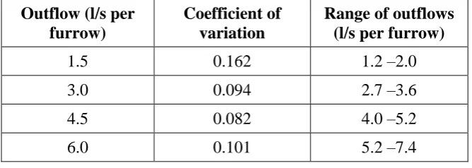
Similarly, increasing the length of the channel, either by increasing the number of furrows supplied or by increasing the spacing (ie, alternate furrow irrigation) of the same number of furrows, will increase the variation in depths and the variation in outflows. For example, alternate furrow irrigation of 50 furrows at 3 l/s (spacing of wetted furrows of 2 m) results in a coefficient of variation (CV) for the outflows of 0.112, compared to the CV of 0.093 for 1 m spacing. Increasing the flow rate in the head ditch by increasing the number of furrows to 100 (at 3 l/s per furrow) results in a CV of 0.209. As is the case of a sprinkler irrigation lateral, increasing the slope of the channel will counter to some degree the effects of any increase in length or increase in flow rate.
Unsteady analysis
The solution for the case of a horizontal channel with a final downstream depth of 0.3 m is presented in Figure 6. Water surface profiles plotted every 2.5 s show the progression of the surge wave down the channel, the gradual dissipation of the wave due to the storage in the channel and the outflow to the furrows, and the reflection of the wave from the downstream end. The steady state profile is reached after about 300 s and closely matches the depth profile from the comparable steady analysis.
Fig 6 about here
The variation of the outflows with time for a sill type outlet is illustrated in Figure 7, where the outflows to furrows at the upstream end, middle, and downstream end of the head ditch are plotted against time. These show considerable variation in the rate of outflow during the first three minutes of the commencement of the irrigation, with the inflows settling to a steady rate within the first 5 minutes. For the very long furrows and hence long irrigation durations commonly used in northern Australia this relatively short period of unsteady inflows will have little impact on the irrigation advance and hence irrigation performance. For shorter furrows and shorter irrigation durations it may be significant.
Fig 7 about here
The main factors influencing the time to reach a steady condition are the volume of the channel and the inflow rate. As was seen in the earlier steady analysis, increasing the volume in the channel by increasing the depth or cross sectional area has the result of increasing the spatial uniformity of the outflows. However it will also result in increased time to reach steady state.
The times to steady state for the inflows in Figure 7 are substantially less than those presented by Renault and Wallender (1996) for the cases of gated pipe and over bank siphons. In these two cases the times were determined not by hydraulic factors but by the time taken to open the gates along the gated pipe or to prime the siphons for each of the furrows. The system analysed in the present paper involves the opening of a single gate. It is presumed that similar times to steady conditions would result for gated pipe if the flow control was a valve at the start of the pipeline rather than at the individual outlets.
the various sections of head ditch vary with time throughout the irrigation and hence the furrow flows also vary over the duration of the irrigation. Prediction of the irrigation advance in the furrows and evaluation of the performance of these systems firstly requires the ability to calculate the time variant flows in the head ditch. That ability is offered by the unsteady channel model presented herein.
Conclusions
Computer programs have been developed for the steady and unsteady analysis of the water surface profiles in and outflows from irrigation head ditches supplying furrow irrigated fields. The study considered the different characteristics of both siphon and sill type application systems.
The analysis of the steady profiles for a typical head ditch show that it is feasible to design head ditches to minimise the variation in outflows along the length of the channel that are caused by the channel hydraulics. The dominant factors were the channel slope, channel depth (or cross sectional area), and the channel discharge. The water surface profiles and the pattern of outflows along the channel showed behaviour very similar to that of the spatially varied pipe flow as seen in gated pipe, with depths and outflows increasing toward the downstream end of the channel. For the case analysed the minimum variation in outflows occurred when the longitudinal slope of the channel was zero.
The unsteady analysis demonstrated the feasibility of predicting the temporal patterns of the outflows. For the constant inflow case modelled, the time to reach steady flow conditions was relatively short and for the long furrows and long irrigation durations typical of furrow irrigation in northern Australia would be inconsequential. Where the inflow to the head ditch varies with time, or where considerable time is taken to start all of the siphons in turn, the temporal variation in the outflows would become significant.
The one significant limitation of the analysis identified during the development of the programs was in the neglect of the (possibly substantial) longitudinal momentum of the lateral outflow. Accounting for this momentum through the inclusion of an additional term in the momentum equation will improve the accuracy of both the steady and unsteady models.
References
Chadwick, A, Morfett, J and Borthwick, M (2004) Hydraulics in Civil and Environmental Engineering. 4th edition, Spon Press, London, 644p.
Chow, VT (1973) Open Channel Hydraulics. International Edition, McGraw-Hill, Singapore, 680p.
Das, A (1997) Spatially varied flow over an embankment side weir. Journal of Irrigation and Drainage Engineering, 123(4): 314-317.
El Awady, MN, El Tantawy, MT, Hassan, SS and El Ashhab, AOM (2003) Water-flow uniformity through irrigation gated-pipes. International Workshop on Improved Irrigation Technologies and Methods: Research, Development and Testing, 18-19 September 2003, Montpellier, France.
Garcia-Navarro, P and Saviron, JM (1992) McCormack’s method for the numerical simulation of one-dimensional discontinuous unsteady open channel flow. Journal of Hydraulics Research, 30: 95-105.
Grabham, MK, Hornbuckle, JW, Raine, SR and Smith, RJ (2008) Observations from initial evaluation trials of bankless channel systems. Irrigation Association of Australia, National Conference, Melbourne, Australia, 20-22 May 2008.
Hood, S and Carrigan, E (2006) Siphon-less irrigation project. Australian Cotton Conference, Proceedings of the 13th Australian Cotton Conference 8-10 August 2006, Gold Coast, Australia
McNown, JS (1954) Mechanics of manifold flow. Transactions of the American Society of Civil Engineers, 119: 1103-1118. Re-published in “Classic Papers in Hydraulics”, ASCE, New York, 1982.
Muslu, Y (2001) Numerical analysis for lateral weir flow. Journal of Irrigation and Drainage Engineering, 127(4): 246-253.
Ramamurthy, AS, Qu, J and Vo, D (2006) Nonlinear PLS method for side weir flows. Journal of Irrigation and Drainage Engineering, 132(5): 486-489.
Renault, D and Wallender, WW (1996) Initial-inflow-variation impacts on furrow irrigation evaluation. Journal of Irrigation and Drainage Engineering, 122(1): 7-14.
Schwankl, LJ, Raghuwanshi, NS and Wallender, WW (2000) Furrow irrigation performance under spatially varying conditions. Journal of Irrigation and Drainage Engineering, 126(6): 355-361.
Smith, RJ (1988) Energy loss in branching flow and its application to irrigation pipeline design. Journal of Agricultural Engineering Research, 41: 181-189.
Smith, RJ (1990) The distribution of water from rigid and lay-flat gated pipe. Proc Australian Society of Sugar Cane Technologists 1990 Conference, Townsville, 56-64. Smith, RJ, Watts, PJ and Mulder, SJ (1986) Analysis and design of gated pipe. Agricultural
Water Management, 12: 99-115.
Trout, TJ (1990) Furrow inflow and infiltration variability impacts on irrigation management. Trans ASAE, 33(4): 1171-1178.
Trout, TJ and Mackey, BE (1988) Furrow inflow and infiltration variability. Trans ASAE, 31(2): 531-537.
Table 1 Variation in outflows (CV) for a sill type outlet and various channel depths and slopes
Slope
Depth (m) -0.0005 0.0 0.0005 0.001
0.20 0.227 0.206 0.204 0.213
0.30 0.101 0.028 0.094 0.174
0.40 0.094 0.014 0.121 0.225
0.50 0.099 0.010 0.120 0.228
0.60 0.103 0.007 0.116 0.225
Table 2 Variation in outflows (CV) for a siphon type outlet and various channel depths and slopes
Slope
Depth (m) -0.0005 0.0 0.0005 0.001
0.20 0.089 0.081 0.081 0.085
0.30 0.035 0.010 0.033 0.062
[image:12.595.155.489.553.672.2]0.50 0.033 0.003 0.040 0.077
Table 3 Variation in outflows for various outflow rates (sill type outlet, 0.3 m downstream depth, 0.0005 slope)
Outflow (l/s per furrow)
Coefficient of variation
Range of outflows (l/s per furrow)
1.5 0.162 1.2 –2.0
3.0 0.094 2.7 –3.6
4.5 0.082 4.0 –5.2
Figure 1 Water depth profiles for the case of 0.3 m downstream depth, sill type outlet, mean outflow of 3 l/s and various slopes
Figure 2 Outflow profiles for the case of 0.3 m downstream depth, sill type outlet, mean outflow of 3 l/s and various slopes
Figure 3 Comparison of outflow profiles for sill and siphon outlets (for the case of 0.3 m downstream depth, mean outflow of 3 l/s and 0.0005 slope)
Figure 4 Relative water depth profiles for the case of 0.0005 slope, sill type outlet, mean outflow of 3 l/s and various depths (where the relative depth is the actual depth expressed as a ratio of the downstream depth)
Figure 5 Water depth profiles for the case of 0.3 m downstream depth, 0.0005 slope, sill type outlet and various mean outflow rates
Figure 6 Progression of the surge wave on filling of the head ditch (water surface profiles are plotted at 5 s intervals)