Evolutionary and ecological genetic patterns of widespread unicornfishes: investigations of the non-geographic clades phenomenon

Full text

(1)ResearchOnline@JCU. This file is part of the following reference:. Horne, John Barton (2011) Evolutionary and ecological genetic patterns of widespread unicornfishes: investigations of the non-geographic clades phenomenon. PhD thesis, James Cook University.. Access to this file is available from:. http://researchonline.jcu.edu.au/38033/ The author has certified to JCU that they have made a reasonable effort to gain permission and acknowledge the owner of any third party copyright material included in this document. If you believe that this is not the case, please contact ResearchOnline@jcu.edu.au and quote http://researchonline.jcu.edu.au/38033/.

(2) Evolutionary and Ecological Genetic Patterns of Widespread Unicornfishes: Investigations of the Nongeographic Clades Phenomenon. Thesis by John Barton Home BSc For the degree of Doctor of Philosophy in Marine Biology Submitted: April 2011. James Cook University School of Marine and Tropical Biology.

(3) Publication list Publications directly resulting from this thesis:. Chapter 2. Horne JB, Mcllwain JL & van Herwerden (2010) Isolation of 15 new polymorphic microsatellite markers from the bluespine unicornfish Naso unicornis. Conservation Genetics Resources, 2, 191-194. Chapter 3 & 4. Horne JB, van Herwerden L, Choat JH & Robertson DR (2008) High population connectivity across the Indo-Pacific: congruent lack ofphylogeographic structure in three reef fish congeners. Molecular Phylogenetics and Evolution, 49, 629-638. Chapter 5. Horne JB, van Herwerden L & Choat JH (In prep) Horizontal gene flow between two Indo-Pacific unicornfish sister species Naso hexacanthus and Naso caesius. Chapter 7. Horne JB, Abellana S, Mcllwain JL, Choat JH & van Herwerden L (In prep) Recruitment patterns of the blues pine unicornfish in the Marianas archipelago. Conceptual Paper. Horne JB, van Herwerden L & Choat JH (In prep) On the phylogeography of widespread ludo-Pacific coral reef dwelling species and perceived barriers to marine dispersal. Publications that arose during the candidature of this thesis. Horne JB, Momigliano P, Welch DJ, Newman SJ & van Herwerden L (2011) Limited ecological population connectivity suggests low demands on self-recruitment in a tropical inshore marine fish (Eleutheronema tetradactylum: Polynemidae). Molecular Ecology, in press. Horne JB, Momigliano P, Welch DJ, Newman SJ & van Herwerden L (in review) Searching for common threads in threadfins: comparative phylogeography of two Australian polynemid fisheries. Marine Ecology Progress Series.. 11.

(4) Acknowledgements I would like to thank the following people, who were either directly or indirectly instrumental to the completion of my research. Crystal Horne: First and foremost I would like to thank my wife Crystal for her unwavering love and support. She is an amazing woman with many talents and qualities that I can only hope to emulate. She made many sacrifices so that I could pursue my doctorate degree here in Australia, not the least of which was working full time so that I could concentrate on school. Moreover, she sat by and watched many of her friends marry men with good jobs, watched them buy "cute" houses while we lived in less than desirable accommodation. She missed weddings and other important events. In particular she chose to stay in Australia and support me when her family back home was going through hard times. No man ever had a better, more loyal wife than mine. Crystal, I love you. Tom and Susan Horne: I consider myselflucky to have had such good parents. All my life my parents have nurtured my interests and endured my obsession with fish. I remember my mother had to replace the carpets in our house because one of the filter hoses on my 55-gallon aquarium came loose. More importantly, however, my parents always taught me to value knowledge and to do what I wanted with my life. Without their direction I don't think I would have pursued the path that has lead me here today. Lynne van Herwerden: I would like to thank my primary supervisor Lynne van Herwerden. Lynne is always very patient, very kind and I sometimes think it would be impossible to frustrate or make her angry. At the same time Lynne is remarkably dependable, always returns my manuscripts with revision in a timely manner and somehow manages to produce papers of her own while supervising 6-9 students. I know that she toils indefatigably behind the scenes though you'd never know how hard she works just from a superficial glance. Lynne has been a superlative example to me in so many ways. I used to worry how I would ever juggle a career as a scientist and a family but Lynne has taught me (by example) how to put my family first and still have a fruitful career. Howard Choat: Oliver Wendell Holmes once likened men unto peaches or pears, saying that they tend to sweeten right before they decay. If that is true then Howard will not decay any time soon. Lynne was my nice supervisor, while Howard was my tough one. Lynne was good cop. Howard was bad cop. I still remember when he told me that my brain had been "fried by the green laser from Mars" and the time he told me that one of my manuscripts was a "self-indulgent ramble" and the time that he sharply asked me if! knew the difference between a noun and a verb. My memories of Howard Choat will forever arouse my sense of humility. I have benefited greatly from Howard's zero tolerance for mediocrity and his no-nonsense attitude. I thank him for having the gumption to tell me that my work was bad even when it very nearly broke my heart to hear it. He held me to a high standard, for which I will always be grateful.. Ill.

(5) Selma Klanten: Selma was my predecessor in Lynne's lab. In fact, her work laid the foundation for my research and paved the way for many of my papers. In many ways I have stood on her shoulders. James Cook University Molecular Ecology and Evolution lab: I remember thinking what a dump the lab was when I first toured it. There were dead bugs everywhere and mold growing on the ceiling. Then the school built a new building to house the MEEL lab and now it is probably one of the nicest labs of its kind in the southern hemisphere. Too bad the move was after I had finished most of my lab work. Regardless, the MEEL lab has been like a home to me and has provided for all my needs. I will always remember sequestering my self there, sometimes for 15 hours at a time. I am especially grateful to the numerous lab managers we've had over the years: Adrian, Di, Stacy, Heather, Blanche. And also a warm thank you to Ainsley Calladine, the Megabace technician, who ran all of my microsatellite samples. Other acknowledgements: I would like to thank the James Cook University international student center for helping and supporting me as an international student. I would like to thank the school of Marine and Tropical Biology and the post-graduate school of research. I would like to thank the University of Guam marine lab, where I spent several weeks, and Jenny Mcllwain, who has been an important collaborator. I would like to thank all sources of funding: the James Cook University internal- . funding scheme and the U.S. Fish and Wildlife's Federal Assistance in Sportfish Restoration Program to the Guam Department of Agriculture. Thank you to all the people who did field work and supplied samples for this research: Sheena Abellana, . Mark Priest, Brett Taylor, Alyssa Marshall, Andrew Halford, JP Hobbs, DR Robertson, W Robbins, M Meekan, BW Bowen, JA Eble and others.. IV.

(6) Abstract. The tropical Indo-Pacific is a very large biogeographic region stretching from the Red Sea to the central Pacific, yet in spite of its size nearly 500 species of shallow water teleost fishes are mostly cosmopolitan throughout this vast region. To date only a small number of these species have been phylogeographically studied across their entire species ranges and most show some genetic population structure, usually between ocean basins. However, some Indo-Pacific coral reef fishes have genetically homogenous populations across the Indo-Pacific suggesting high levels of gene flow. Among those fishes that lack spatial population partitions some possess nongeographic or temporal population structures in the mtDNA. This means that their populations are composed of genetically differentiated lineages that are sympatrically distributed. The biological significance of this pattern is unclear and only a small number ofreeffish taxa have been reported to have non-geographic clades. The first species in which this pattern was detected was the big nose unicornfish, Naso. vlamingii, which is a widespread Indo-Pacific Acanthurid with a long pelagic larval duration (Klanten et al. 2007). The explanation given by Klanten et al. for the nongeographic clades of this species was temporary periods of isolation, mediated by low-sea-level barriers and followed by secondary contact and admixture of lineages. Yet, while the conclusions of Klanten et al. (2007) seem plausible, further investigation into non-geographic genetic patterns was warranted. In this thesis four additional Naso species were phylogeographically surveyed at a broad scale across the Indo-Pacific: Naso brevirostris, Naso unicornis, Naso. hexacanthus and Naso caesius. Like N. vlamingii, all species showed little in the way of spatial population structuring using conventional phylogeographic fixation indexes. v.

(7) (F,,). Model-based phylogenetic analysis, maximum parsimony and Bayesian. inference revealed non-geographic population patterns in the mitochondrial control region with N brevirostris being the most similar to N. vlamingii. Curiously, the sister species N hexacanthus and N caesius were not reciprocally monophyletic suggesting that some horizontal gene transfer has occurred between them. Expansion time based on mismatch distributions was also calculated for each species and each clade. Mismatch coalescence suggests mid-late Miocene expansion times for all taxa (considering N hexacanthus and N caesisus as a single taxon) and pre-Pleistocene expansion for non-geographic clades. Coalescence age of species and clades was also assessed in the program BEAST using a fossil calibrated molecular dating and a relaxed molecular clock. For this analysis all Naso species previously mentioned, including N. vlamingii, were arranged into an interspecific phylogeny of cytochrome oxidase subunit one DNA sequences, with many representatives of each species and clade. Mean ages from this anaylsis suggest mid-miocene coalescence ages for each taxa and pre-Pleistocene coalescence for all non-geographic clades, indicating that Pleistocene processes probably do not account for non-geographic patterns in the genus Naso. Otherwise, little congruence could be found between the ages of clades, seemingly refuting the notion that a barrier was involved in the formation of these genetic features. Fossil calibrated coalescence ages were used to reconstruct demographic history of each species using Bayesian skyline plots. In all taxa, skyline plots suggest accelerated demographic expansion during the Pleistocene, rather than the bottlenecks or demographic decline expected based on the pretext that reef fishes suffered bottlenecks during the upheavals on coral reefs during the Pleistocene glacial cycles. Complimentary to evolutionary genetic patterns, this thesis also includes a genetic survey of recently settled N unicornis juveniles in the Marianas archipelago,. VI.

(8) using 12 polymorphic microsatellite loci and sequences from the mitochondrial control region. This particular study reveals that post-settlement larval pools of N. unicornis have an elevated genetic diversity in both the nuDNA and mtDNA relative. to the preexisting adult population. Recruitment events are genetically unstructured in space and time in this species within the Marianas and recruits seemed likely to have sibling relationships among sampling locations and between year classes. The genetic diversity of larval pools, as well as the likelihood of sibling pairs to be separated in space and time suggests demographically open populations. In light of the phylogeography of this species, N. unicornis and its congeners most likely experience high levels of gene flow on ecological as well as evolutionary time frames. Non-geographic clades appear to be a genetic phenomenon observed in some widespread and highly dispersi_ve coral reef fishes of the lndo-Pacific. There was little evidence to suggest that a low-sea-level barrier to gene flow was associated with these clades. Most likely non-geographic clades arise as a consequence of rapid range expansion across patchily distributed coral reefhabitat in a large biogeographic region. The sheer size of the Indo-Pacific appears to be an important factor shaping the population patterns of widespread cosmopolitan coral reef fishes.. Vil.

(9) Table of Contents Title Page Publication list Acknowledgements Abstract Table of Contents List of Tables List of Figures. v. CHAPTER 1 Introduction to Coral Reef Fish Studies 1.1 Speciation, Phylogeography and Marine Barriers 1.2 Chapter outline. 1. 11 111. VllI XI. XII. CHAPTER 2 Lab Methods 2.1 Field collections 2.2 DNA extraction 2.3 Mitochondrial Control Region 2.4 Cytochrome Oxidase Subunit 1 2.5 Microsatellite Markers for Naso unicornis: Development and PCR Parameters CHAPTER 3: Broad-scale Phylogeography of Naso brevirostris 3.1 Introduction 3.2 Methods 3 .2.1 Samples 3.2.2 Phylogenetic analysis 3.2.3 Population genetic analysis 3.2.4 Demographic expansion 3.3 Results 3.3.1 Diversity 3.3.2 Phylogenetic analysis 3.3.3 Population structure 3.3.4 Demographic expansion 3.4 Discussion 3.4.1 Congruence with N. vlamingii 3.4.2 Spatial patterns 3.4.3 Non-geographic clades 3.5 Conclusion CHAPTER 4: Broad-scale Phylogeography of Naso unicornis 4.1 Introduction 4.2 Methods 4.3 Results 4.3. l Diversity 4.3.2 Phylogenetic analysis 4.3.3 Population structure 4.3.4 Demographic history 4.4 Discussion 4.4.1 Spatial patterns 4.4.2 Non-geographic clades 4.4.3 A lost expansion signal viii. 8. 12 15 15 16. 22 24 25. 26 26 28 28 30 32 34 34 35 39 41 41 42 42 44. 47 49 51. 54.

(10) 4.5 Conclusion CHAPTER 5: Broad-scale phylogeography of sympatric sister species: Naso hexacanthus and Naso caesius 5.1 Introduction 5.2 Methods 5.3 Results 5.3. l Diversity 5.3.2 Phylogenetic analysis 5.3.3 Population structure 5.3.4 Demographic history 5.4 Discussion 5.4.1 Non-monophyly 5.4.2 Spatial patterns 5.4.3 Non-geographic clades 5.5 Conclusion CHAPTER 6: Molecular dating of non-geographic clades 6.1 Introduction 6.2 Methods 6.2.1 Phylogenetic comparisons of species and clades 6.2.2 Molecular dating 6.2.3 Bayesian skyline plots 6.3 Results 6.3.1 Phylogenetics results 6.3.2 Molecular dating of deep phylogenetic nodes and species divergences 6.3.3 Molecular dating of species ages 6.3.4 Molecular dating-of non-geographic clade ages 6.3.5 Bayesian skyline plots 6.4 Discussion 6.4.1 Molecular evolution, mtDNA and comparative studies 6.4.2 The Oligocene and Miocene 6.4.3 Non-geographic clades and the Pleistocene 6.4.4 Naso hexacanthus and Naso caesius 6.5 Conclusion CHAPTER 7: Recruitment patterns of Naso unicornis in the Marianas Archipelago 7.1 Introduction 7.2 Methods 7.2.1 Field collections on Guam 7.2.2 Laboratory procedures 7.2.3 Genetic analysis ofmtDNA 7.2.4 Summary statistics, tests of Hardy-Weinberg equilibrium and linkage disequilibrium of microsatellite loci 7.2.5 Discriminant analysis of principle components 7.2. 6 Parentage analysis and tests of relatedness 7.3 Results 7.3.1 Molecular diversity 7.3.2 Relatedness and parentage analysis 7.3.4 Discriminant analysis of principle components 7.4 Discussion 7.4.1 Comparisons with previous studies. IX. 56. 57 59 59 60 60 63 64 65 68 69 70 72 73 75 76 78 78 79 81 84 85 87 90 91. 93 97 99 99 100 100 102 103 107 112 117.

(11) 7.4.2 Self-recruitment and external recruitment. 7.S Conclusion CHAPTER 8: Discussion and Synthesis of research 8.1 Introduction 8.2 Main contributions 8.3 Discussion and conclusions 8.4 Final conclusions REFERENCES. x. 119 121 122 122 125 129 131.

(12) List of Tables Table 2.1: Mitochondrial Primers Table 2.2: Microsatellite Primers Table 3.1: Pair wise F,, (N. brevirostris) Table 3.2: AMOVA fixation indices (N. brevirostris) Table 4.1: Pair wise F,, (N. unicornis) Table 4.2: AMOVA fixation indices (N. unicornis) Table 5.1: Pair wise F,, (N. hexacanthus + caesius) Table 5.2: AMOVA fixation indices (N. hexacanthus + caesius) Table 6.1: Fossil calibrated molecular dating Table 7 .1: MtDNA diversity indices for N. unicornis recruits Table 7.2: Control region pair wise F,, (N. unicornis recruits) Table 7.3: Hardy-Weinberg equilibrium Table 7.4: Microsatellite diversity indices for N. unicornis recruits Table 7.5: Microsatellite pair wise F,1 Table 7.6: Putative sibling pairs list. XI. 16 20 31 31 46 46 62 63 81 104 105 106 107 108 112.

(13) List of Figures Figure 2.1: Sample collections (N. brevirostris) Figure 2.2: Sample collections (N. unicornis) Figure 2.3: Sample collections (N. hexacanthus and N. caesius) Figure 2.4: Sample collections of N. unicornis recruits Figure 3.1: Control region genealogy and haplotype network clad es (N. brevirostris) , Figure 3.2: Clade mismatch distributions (N. brevirostris) Figure 4.1: Control region gene genealogies (N. unicornis) Figure 4.2: Control region haplotype network (N. unicornis) Figure 4.3: Mismatch distributions (N. unicornis) Figure 5.1: Control region genealogy and haplotype network clad es (N. hexacanthus + N. caesius) Figure 5.2: Mismatch distributions (N. hexacanthus + N. caesius) Figure 5.3: Longitudinal nucleotide diversity Figure 6.1: Multi-species COi genealogy Figure 6.2: Multi-species COi chronogram Figure 6.3: Bayesian skyline plots Figure 7.la: Pair wise relatedness distributions, N. unicornis adults and recruits Figure 7.lb: Pair wise relatedness distributions, N. unicornis recruitment sites Figure 7.2: DAPC scatterplot, N. unicornis adults and recruits Figure 7.3: DAPC scatterplot, N. unicornis recruitment sites Figure 7.4: Microsatellite genetic clusters Figure 7.5: Discrimination of genetic clusters. xii. 13 13 14 14 29 33 43 45 48 61 64 67 77. 80 82-83 -109 llOlll ll4 ll5 ll6 ll6.

(14) Chapter One Introduction to Coral Reef Fish Studies. 1.1 Speciation, Phylogeography and Marine Barriers. Fishes found on coral reefs have an impressive taxonomic diversity. Springer (1982) estimated there were 4,000 species of reef and shallow water fishes in the IndoPacific alone, though he suspected this number might be “much too low.” Choat & Bellwood (1991) claimed that 4,000 species would comprise 18% of all fish species known at the time (roughly 22,000). In the past few decades, the number of described fish species has increased dramatically. According to Eschmeyer & Fricke (2009) the tally for total fish species has grown to over 31,000. If we assume that the number of described reef fishes has increased proportionally, we might, by way of crude extrapolation, approximate the number of reef fishes known currently to be about 5,600 species. Rocha & Bowen (2008 & references therein) also estimate the number of described reef fishes to be about one third of ~15,000 marine fishes. Considering that there are only about 5,000 living mammal species total (Wilson & Reeder 2005), the study of reef fishes is not only a massive scientific undertaking but also key to understanding the natural mechanisms that produce and sustain vertebrate biodiversity. The fossil record reveals that the higher taxonomic groups of modern reef fishes first appeared and diversified early in the Cenozoic. The oldest benthic marine fish fossils that resemble modern day reef fish communities come from the lower middle Eocene deposits in Monte Bolca, Italy, where 247 fossil fish species from 82 families and 17 orders have been reported (Bellwood 1996). A large number of the. 1.

(15) families present at Monte Bolca have extant representation on modern coral reefs and many fossils have skeletal morphologies that are highly similar to present-day species. Bellwood & Wainwright (2002) express that the Eocene Tethys Sea fish faunas in the Bolca region would have differed little in appearance and ecology from those seen in the tropics today. Since the Eocene there has been a major shift in the biogeography of reef fishes. Obviously there are no longer coral reefs or reef fishes in northern Italy. Today the greatest biodiversity of fishes, corals and other reef denizens are found in the Indo-Australian Archipelago (IAA) but diverse assemblages of reef fishes are found in all tropical oceans with multiple centers of high endemicity (Randall 1998; Bellwood & Wainwright 2002; Allen 2008). The question asked by biogeographers is when did the present-day provinciality of reef fishes emerge and what were the factors that shaped it? Many present-day reef fishes have long species histories that originate in the Miocene (23-5 Ma) (e.g. Bellwood et al. 2004; Bernardi et al. 2004; Klanten et al. 2004; Read et al. 2006; Dornburg et al. 2008; Cowman et al. 2009; Bellwood et al. 2010). If the initial great diversification of reef fishes happened in the Eocene, then the second great diversification was in the Miocene, at which time Renema et al. (2008) conclude that the new biodiversity hotspot in the IAA was established. But what were the evolutionary processes that promoted high levels of speciation starting in the Miocene and continuing on until the present day? Speciation in its simplest form occurs across a geographic barrier, which prevents genetic exchange between two populations and allows them to diverge. This allopatric mode of speciation is presumed to have given rise to the majority of species on our planet, or has at least been the most documented (Coyne & Orr 2004).. 2.

(16) Freshwater habitats, in particular, are intrinsically separated by allopatric barriers, which may account for the immense species diversity of freshwater fishes (Wiley 2002). The ocean, conversely, is a relatively homogenous environment and has few absolute barriers that would prevent migrant exchange in highly dispersive marine species. It is, therefore, difficult to invoke strict allopatry to explain marine biodiversity (Palumbi 1994), except in cases where it is unmistakable, such as across the Isthmus of Panama (see Lessios et al. 2008). Therefore, other models of speciation and more complex mechanisms of isolation must be considered to satisfactorily explain the species richness that exists on coral reefs and in other marine environments. Alternatives to strict allopatric speciation include ecological speciation (sympatry), partial geographic isolation (parapatry) and peripheral isolation (peripatry) (see Palumbi 1994; Choat 2006; Rocha & Bowen, 2008; Puebla 2009). Models that predict speciation processes may be tested using a molecular approach, in which the genetic patterns that arise in selectively neutral gene regions are assessed. Neutral molecular markers may develop random polymorphic characters, which can be treated as a genetic signature of a population. Under the assumption of neutrality, two forces act upon such genetic signatures: gene flow and genetic drift (Slatkin 1987). Populations that regularly exchange genes through migration will eventually have their genetic signatures come to resemble each other. Alternatively, if populations are reproductively isolated, they will genetically drift apart and may eventually become different species. The structure and phylogeny of populations in a drift-equilibrium context indicates where barriers to gene flow have occurred, spatially or along an ecological gradient, and to what degree populations are genetically connected. This research method is often referred to as. 3.

(17) phylogeography (Avise et al. 1987; Avise 1998) and is particularly useful for studying dispersive marine organisms, where population boundaries are often not obvious (Palumbi 1994; Hellberg 2007). In recent years, genetic studies have shed considerable light on speciation process in the sea and its complexity. Several examples of ecological and sympatric speciation have been documented for marine fishes (Munday et al. 2004; Rocha et al. 2005a; Puebla et al. 2007; Wellenreuther et al. 2008; Hyde et al. 2008; Crow et al. 2010). However, speciation in sympatry is controversial (Coyne & Orr 2004) and difficult to demonstrate conclusively because the species ranges at the time of speciation are usually unknown (Bolnick & Fitzpatrick 2007). Even some good cases may not satisfy the strictest criteria prescribed to demonstrate sympatric speciation (Elmer & Meyer 2010). Peripatric isolation also appears to be an important driver of divergence in coral reef fishes (Gaither et al. 2010; Winters et al. 2010; Craig et al. 2010; Leray et al. 2010; DiBattista et al. 2011). Yet perhaps the best examples of peripatric speciation come from marine invertebrates (Budd & Pandolfi 2010; Malay & Paulay 2010). High levels of endemism of reef fishes at peripheral locations (Randall 1998; Allen 2008) might suggest peripatric speciation but endemism does not necessarily equate to speciation (Bellwood & Meyer 2009). The potential for parapatric speciation in marine environments, in the form of soft or invisible oceanic barriers is becoming increasingly noted by marine researchers (Palumbi 1994; Rocha & Bowen 2008). Parapatry is difficult to distinguish from allopatry because the resulting biogeographic pattern is essentially the same (Coyne & Orr 2004). However, as Turelli et al. (2001) explain, any mechanism that can produce speciation in allopatry will do the same in parapatry, if the geographic scale is large enough. Considering the immense size of the marine. 4.

(18) environment and the apparent paucity of absolute barriers, parapatry is likely to be common in the ocean. The abundance of soft barriers (i.e. stretches of water that have properties that restrict connectivity between separated populations) in the ocean is not readily apparent but there are a few soft barriers that are conspicuous. These include the East Pacific Barrier (EPB), the Benguela Barrier (BB), the Amazon Barrier (AB) and the Indo-Pacific or Sunda Shelf barrier (IPB) (reviewed by Rocha et al. 2007). Soft barriers are, by nature, penetrable, to certain degrees, at certain times, or by certain species. The cold Benguela current that forms the BB, for example, normally segregates the fish faunas of the tropical Atlantic and West Indian Ocean. However, this barrier may have historically been subject to disturbances that have allowed colonizations of the Atlantic by Indian Ocean species (Rocha et al. 2005b; Bowen et al. 2006; Floeter et al. 2008). In another example, the EPB is a 5,000 km expanse of ocean that segregates the benthic faunas of two marine biogeographic provinces: the coastal Americas and the reef habitats of the Central Pacific (Bellwood & Wainwright 2002). Yet some reef fishes, such as the Acanthurid Acanthurus triostegus, have high genetic connectivity between the East and Central Pacific and are thought to regularly migrate across the EPB (Planes & Fauvelot 2002; Lessios & Robertson 2006). Therefore soft barriers may not be barriers at all to some species and may be more accurately described as filters. Rare dispersal across these filters and or fluctuations in their effectiveness appears to lead to speciation events in reef fishes (Floeter et al. 2008). Considering that semi-allopatric soft barriers may create opportunities for speciation, it seems intuitive that there would be a soft barrier associated with the IAA biodiversity hotspot. In deed, a barrier does seem to operate between the. 5.

(19) tropical Indian and Pacific, for although both oceans are faunistically similar, a large number of reef fishes are geographically confined to one ocean or the other (Springer & Williams 1990; Randall 1998) and there is growing data on a biogeographic suture zone between the two oceans (Hobbs et al. 2009). Phylogeographic studies also show that reef fishes found throughout the Indo-Pacific have deep genetic population partitions coinciding with a barrier somewhere in the IAA (Planes & Fauvelot, 2002; Bay et al. 2004; Craig et al. 2007; van Herwerden et al. 2009; Leray et al. 2010; Eble et al. 2010). The presence of such a barrier is puzzling because, unlike the BB and EPB, the mechanism that separates Indian and Pacific reef fish populations is not immediately obvious. One might expect the IAA, with its continuous warm water and abundant reef habitat to facilitate migrant exchange between oceans rather than suppress it. Nevertheless, for at least one widespread species (Myripristis berndti), the IPB appears to be a more effective barrier to dispersal than the EPB (Craig et al. 2007). Given the geographic and oceanographic complexity of the IAA, multiple factors most likely act in concert to create the effect of the IPB. For some taxa, with lower dispersal abilities, such as many marine invertebrates, inter-oceanic dispersal is probably hindered by ocean circulations that operate in this area (Barber et al. 2006; Carpenter et al. 2011). But most authors have proposed that the major biogeographic effect of the IPB is caused by eustatic sea level changes in relation to the Indonesian Sunda Shelf (Springer & Williams 1990; Randall, 1998; Benzie 1999; Carpenter et al. 2011). This submerged continental shelf is the largest on Earth outside of the Polar Regions and comprises an area approximately 1.8 x 106 km2 (Hanebuth et al. 2000). During low extremes in sea-level, most of this land mass would have been above water, reef habitat within the IAA would have been. 6.

(20) drastically reduced and the coastline of the Sunda Shelf would have become a large obstacle for dispersing marine organisms. Still, even when sea-level falls 120 m below current levels, the tropical Indian and Pacific are connected by a large seaway (Voris 2000), the Indo-Pacific throughflow, which should permit some inter-oceanic migrant exchange. Indeed, some taxa show high genetic connectivity across the IPB (Lessios 2003; Klanten et al. 2007; Gaither et al. 2010; Reece et al. 2010). Therefore, the forces that create the IPB may be attenuated by dispersal ability, life history characteristics or chance migrations. A recent development in the phylogeography of coral reef fishes is the presence of non-geographic or temporal clades. This genetic phenomenon was first observed in a widespread Indo-Pacific surgeonfish, Naso vlamingii, which had four well-defined clades that were sympatrically distributed rather than reciprocally monophyletic across a barrier (Klanten et al. 2007). The interpretation of this pattern was that anciently a barrier between the Indian and Pacific Oceans separated N. vlamingii populations. Subsequently, the barrier has disappeared and introgression, followed by high levels of inter-oceanic gene flow, has erased the ancient population boundary between oceans, though a genetic partition remains. Such an interpretation is consistent with a fluctuating sea-level barrier in the IAA and because there are more than two clades, isolation across this barrier would have occurred multiple times. Non-geographic structuring of genetic lineages appears to be directly related to soft ocean barriers and therefore relevant to the parapatric processes that cause population differentiation and speciation in marine organisms. In fact, Klanten et al. (2007) speculated that non-geographic clades might be sympatrically distributed cryptic species. But what biological features set N. vlamingii apart from other marine. 7.

(21) organisms such that the genetic patterns it exhibits would be so drastically different? Klanten et al. (2007) gave two reasons why this might be the case. 1) A lengthy pelagic larval duration and a larval ecology that would give N. vlamingii a high dispersal potential, even for a coral reef fish. Elevated dispersal would enable previously isolated populations to come into secondary contact after periods of isolation, thus resulting in widely overlapping lineages. 2) A semi-pelagic adult ecology, which would allow this species to utilize a variety of habitats and food sources. Such ecology would enable N. vlamingii to maintain large refuge populations in isolation, even during the suboptimal climatic conditions, such as glacial maxima. These populations would later expand to become geographically overlapping lineages. However, at the time this research thesis commenced N. vlamingii was the only known example of non-geographic clades and the suspicions of Klanten et al. lacked corroboration. Therefore much more work was required to explore these unusual genetic patterns.. 1.2 Chapter outline In the wake of Klanten et al. (2007), the broad-scale phylogeography of N. vlamingii, several questions remain unanswered:. 1. Are the non-geographic genetic patterns present in N. vlamingii unique to this species?. 2. Is a semi-pelagic ecology key to the formation of non-geographic clades?. 3. Are non-geographic clades cryptic species?. 4. Are non-geographic clades the result of temporal isolations across an ephemeral low-sea-level barrier? If so, how long ago did the barrier exist?. 8.

(22) 5. Does non-geographic structure imply elevated levels of dispersal, i.e., frequent long distance migrant exchange as opposed to evolutionary genetic connectivity?. The aim of this thesis was to address each of these questions by conducting additional phylogeographic surveys on other members of the genus Naso and to explore spatial and temporal genetic patterns in this genus using a variety of molecular approaches.. Chapter 2: Methods The purpose of chapter to is to act as a general methods section for field and laboratory work. Included in this chapter is also a description of the protocol I used to develop microsatellite loci for Naso unicornis.. Chapter 3: Broad-scale phylogeography of Naso brevirostris Are the non-geographic genetic patterns present in N. vlamingii unique to this species? Because N. vlamingii was the only species known to possess non-geographic clades there is a possibility that the unusual patterns observed are stochastic in nature. The purpose of chapter three was to attempt to find another example of non-geographic structuring through a broad-scale phylogeographic study of a similar species Naso brevirostris using the methods of Klanten et al (2007). Both species are phylogenetically allied and have long species histories (Klanten et al. 2004), both have semi-pelagic habitat preferences and both forage on filamentous green algae. 9.

(23) and gelatinous zooplankton (Choat et al. 2002). For these reasons N. brevirostris was chosen as the first species to be examined.. Chapter 4: Broad-scale phylogeography of N. unicornis Is a semi-pelagic ecology key to the formation of non-geographic clades? Chapter four is a broad-scale phylogeographic study of N. unicornis. Like N. vlamingii and N. brevirostris this species is widespread in the Indo-Pacific and has a long species history but is primarily benthic in its habitat preferences and has a diet dominated by brown macroalgae (Choat et al. 2002). The purpose of this chapter was to determine whether a Naso species without semi-pelagic ecology would also show non-geographic patterns.. Chapter 5: Broad-scale phylogeography of widespread sympatric sister species: Naso hexacanthus and Naso caesius Are non-geographic clades cryptic species? Chapter five is a broad-scale phylogeography of Naso hexacanthus and Naso caesius, which are two, ecologically very similar, sister species. They are so similar that they sometimes form heterospecific schools and forage together (Randall 2002). They are semi-pelagic, like N. vlamingii and N. brevirostris, but unlike the other species examined, which have long species histories, N. hexacanthus and N. caesius are purported to have diverged relatively recently (Klanten et al. 2004). In reality, the relationship between these two sister species may be analogous to the nongeographic clades found in other species. If so, the genetic differentiation between them should be similar to non-geographic clades and it might be concluded that nongeographic structures is grounds for cryptic speciation.. 10.

(24) Chapter 6: Molecular dating of non-geographic clades Are non-geographic clades the result of temporal isolations across an ephemeral low-sea-level barrier? If so, how long ago did the barrier exist? The purpose of chapter six was to construct a phylogenetic tree containing all species and all clades, in which the nodes can be dated using a fossil calibration. In addition to the mismatch based expansion times of Klanten et al. (2007) and previous chapters, fossil calibrated molecular dating will illuminate the evolutionary history of non-geographic clades and the conditions under which they were formed.. Chapter 7: Recruitment patterns of Naso unicornis on Guam Does non-geographic structure imply elevated levels of dispersal, i.e, frequent long distance migrant exchange as opposed to evolutionary genetic connectivity? Chapter seven is an assessment in recruitment patterns in N. unicornis in the Marianas Archipelago, using 12 nuclear microsatellite loci. In connection with phylogeographic patterns, which indicate the scale of gene flow on an evolutionary time scale, recruitment patterns will indicate dispersal processes on an ecological time scale.. Chapter 8: Discussion and Synthesis of research Chapter eight is a discussion on the main conclusions and contributions of this thesis and centers around the population processes that lead to the formation of nongeographic clades, the evolutionary history of the study taxa and the dispersal ability of Naso.. 11.

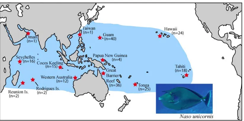
(25) Chapter Two Field and Laboratory Methods. 2.1 Field Collections. The specimens used in this research come mostly from the tissue library of Howard Choat and were sampled from a broad range of geographic localities within the tropical Indo-Pacific between March 2000 and December 2009. The species used in this research were: Naso brevirostris (n = 102), Naso unicornis (n = 196), Naso hexacanthus (n = 92), Naso caesius (n =25) and Naso vlamingii (n = 30). Primarily these samples originated from the Seychelles Islands, Cocos Keeling, Christmas Island (Indian Ocean), Western Australia, the Australian Great Barrier Reef, Solomon Islands, New Guinea, the Philippines and French Polynesia. A small number of samples came from other locations, such as Oman, Taiwan, Rodriguez and Reunion Island. Samples were collected by spearing or purchased in fish markets and stored in either 80% ethanol or a 20% di-methyl-sulfoxide buffer (see Figures 2.1; 2.2; 2.3). Additionally, some sampling was done independent of the Choat collection. N. unicornis was intensely sampled from the island of Guam, in cooperation with the Jennifer McIlwain lab of the University of Guam, between June 2008 and November 2009 (Figure 2.4). From Guam 176 adults and 394 newly settled recruits from five different sites were collected. Twenty-four N. unicornis (adults) from Hawaii were donated from the Brian Bowen lab at the Hawaii Institute of Marine Biology. Thirty more were purchased at fish markets in Nuku’alofa, Tonga. Eleven N. hexacanthus and 9 N. caesius were also purchased at markets in Tonga. All of the above samples. 12.

(26) were placed in 80% ethanol, directly following sampling, for transport and storage. All sampling was conducted under James Cook University ethics approval numbers A503, A872.04 and A1539. .. Figure 2.1: Sample collections of N. brevirostris at seven locations across the IndoPacific.. Figure 2.2: Sample collections of N. unicornis at 13 locations across the IndoPacific.. 13.

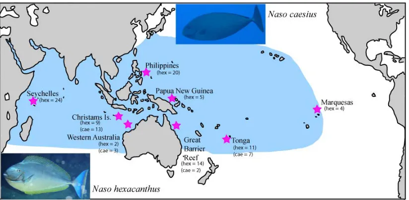
(27) Figure 2.3: Sample collections of N. hexacanthus at eight locations and N. caesius at four locations across the Indo-Pacific.. Figure 2.4: Sampling locations of recently settled N. unicornis recruits from Guam and Saipan.. 14.

(28) 2.2 DNA extraction Total genomic DNA was extracted from fin clips using a salt chloroform protocol (Sambrook et al. 1989) or a Chelex extraction method (Walsh et al. 1991).. 2.3 Mitochondrial Control Region Klanten et al. (2007) designed genus specific mitochondrial control region (control region) primers for the broad-scale N. vlamingii phylogeography. These same NAI primers were employed to amplify this gene region in the other Naso species (Table 2.1). This gene is useful for phylogeography because it is non-coding and hypervariable (Mortiz et al. 1987) and should allow for the detection of subtle genetic signatures not found in other markers, particularly in population level analyses (AMOVA, mismatch distributions etc.). PCR parameters for these primers are as follows: DNA was amplified in 20 µL PCR reactions containing 2.5 mM Tris– Cl (pH 8.7), 5 mM KCL, 5 mM (NH4)2SO4, 200 µM each dNTP, 3.5 mM MgCl2, 10µM each primer, 1 U of Taq Polymerase (Qiagen Ltd.) and 1-10 ng of template DNA. Thermocycling was carried out with an initial denaturation of 94 ˚C for 2 min, 35 cycles of denaturation, annealing and extension (94 ˚C for 30 s, 50 ˚C for 30 s, 72 ˚C for 90 s) and a final extension of 72˚C for 10 min. PCR products were confirmed by gel electrophoresis on 1.5% agarose gels and purified by either a standard isopropanol purification or an ammonium acetate ethanol clean-up. PCR products were sequenced with the NA1 forward primer using ABI (Applied Biosystems Incorporated) technologies at Macrogen sequencing service Seoul, South Korea.. 2.4 Cytochrome Oxidase Subunit 1 The relatively conserved, gene encoding cytochrome oxidase subunit 1 (COI) region. 15.

(29) was also amplified for each species and a gene tree constructed for the purpose of divergence dating (chapter 6). The COI marker was chosen for this analysis for several reasons: 1) because it is more conserved than control region and therefore less prone to saturation. 2) COI has a greater range of phylogenetic signal than any other mitochondrial gene and is useful at both the species and population levels (Herbert et al. 2003; Hellberg 2009). 3) The universal COI primers work well, nearly always yielding strong PCR products. 4) As the designated barcode gene (Herbert et al. 2003) there are many genbank references to which comparisons may be made. COI was amplified using universal primers developed for fish by Ward et al. (2005) (Table 2.1). PCR parameters for these primers were as follows: 2 µL of 10x Pfu PCR buffer, 200 µM of each dNTP, 0.2 µM of each primer (Table 2.1), 0.2 U Pfu DNA polymerase (Promega, Madison, Wisconsin). Table 2.1: Mitochondrial marker primers for the mitochondrial control region and cytochrome oxidase subunit 1 with the accompanying oligonucleotide sequences, annealing temperatures and magnesium concentration. Primer Name Oligo Sequence Ta MgCl2 F 5’-AGCATTCTGAACTAAACTAC NAI 50˚C 3.5mM (Control Region). R 5’- TGTCCCTTGACTCTCAATA. Fish 1. F 5’- TCAACCAACCACAAAGACATT GGCAC R 5’-TAGACTTCTGGGTGGCCAAAGAATCA. (COI). 55˚C. 1.55.5mM. 2.5 Microsatellite markers for Naso unicornis: development and PCR parameters Phylogeographic patterns such as population-structure, genetic diversity indices and mismatch distributions reveal population dynamics primarily over evolutionary time. Genetic patterns that are relevant to demographic processes on a recent time scale are not easily detected in the mutations of nucleotide sequence data and in most cases these ecological signals appear as “background noise” in a drift-equilibrium context. 16.

(30) (Hellberg 2007). Microsatellite loci are hypervariable markers that may be employed in a number of highly sensitive population level analyses such as assignment tests, parentage analysis, mixture and admixture analysis (Manel et al. 2005). The merit of microsatellite loci for answering questions of demographic connectivity is found in their amalgamation. Individually, each locus is no more informative than any other type of marker but as suites of independently assorted loci the possibility of two populations having the same allelic frequencies by chance alone is very unlikely. Thus, the more unlinked loci used the more sensitive the analysis becomes. In recent years these microsatellite loci have become increasingly sought after for studying coral reef fish species, which often have large geographic ranges and complex patterns of population connectivity at varying spatial scales (Purcell et al. 2006; Thacker et al. 2007; Hepburn et al. 2009; Planes et al. 2009). However, compared to the diversity of reef fishes, the number of published microsatellite loci available to coral reef fish biologists is few and at the time that this thesis began, no microsatellite loci had been developed for any Acanthurid. Therefore, it became necessary to develop novel microsatellite loci for Naso and the magnetic bead capture protocol of Glenn & Schable (2005) was used to this end. We extracted total genomic DNA from fin clips of three N. unicornis adults collected from the Seychelles, Lizard Island (Great Barrier Reef) and Tonga. Tissue was digested with proteinase K and DNA extracted using a salt-chloroform method (Sambrook et al. 1989). Total genomic DNA was digested into 300-1000 bp fragments using the restriction enzymes Rsa I and Hae III separately. Double stranded SNX linkers were ligated to both sides of the blunt ended fragments using T4 DNA ligase, in accordance to the protocol of Glenn & Schable (2005).. 17.

(31) Linker ligated DNA fragments were PCR amplified using the super SNX-24 primer and subsequently annealed to four different combinations of biotinylated oligo probes of di, tri and tetra-nucleotide motifs [(AG)16 + (AC)16, (AAG)8, (AAAC)6 + (AATT)8, (AAGG)6 + (AGCG)4]. Reaction mixtures consisted of 25 µL 2x hyb solution, 10 µL mixed oligos (1 µM each), 10 µL linker ligated DNA, 5 µL nuclease free H2O for a total volume of 50 µL. Thermocycler temperatures for the annealing of probes were as follows: 95˚C for five minutes, 70˚C for five seconds followed by 99 five-second incremental step downs of 0.2˚C and 50˚C for 10 minutes followed by 20 five-second incremental step down of 0.5˚C. 50 µL of Streptavidin bonded magnetic beads (Dynabeads, Invitrogen Dynal, Olso, Norway) were washed twice in 250 µL of TE buffer, twice in 1x hyb solution and suspended in a final volume of 150 µL 1x hyb solution. The hybridized DNAoligo fragments were added to the magnetic bead solution and captured with a magnetic particle separator, while the supernatant and miscellaneous DNA was discarded. Microsatellite enriched DNA was again PCR amplified using the super SNX24 primer and ligated into the pCR®2.1-TOPO vector (Invitrogen) as per the manufacturer’s instructions. Cloned inserts were sent to the Australian Genome Research Facility at the University of Queensland, Brisbane for bacterial transformation and sequencing with universal M13 primers. The resulting DNA sequences were screened for microsatellite loci in the program MSATCOMMANDER (Faircloth 2008) and primers for each locus were designed in the same program. A total of 71 loci were detected and the 38 best (those with the longest number of repeats) were chosen for further screening. Loci were amplified in a minumum of five individuals using standard PCR parameters as. 18.

(32) described above (see also Table 2.2). Polymorphism was tested by direct sequencing, which revealed high sequence variation, within loci and in the flanking regions. Additionally, length variation was not consistently uniform across loci, with many alleles differing in length by single base pairs due to small indels in the flanking sequences. Most of the microsatellite loci of N. unicornis could be described as imperfect or compound, as many had different repetitive elements adjacent to each other or were bisected by non-repeating base pairs. Though not optimal for microsatellite analysis, the excessive amount of polymorphism observed in the nuclear genome of N. unicornis is consistent with mitochondrial studies which show high genetic diversity in this and other Naso species (e.g. Naso vlamingii Klanten et al. 2007). The 15 cleanest (those with fewest indels) and most polymorphic loci were screened against 90 adult N. unicornis (114-485mm FL) collected from Guam in the tropical West Pacific (Table 2.2). The genbank accession numbers for these loci are: GU189390-GU189404. Sample DNA was PCR amplified using forward primers that were flurolabeled with either HEX, TET or FAM dyes (Geneworks pty. Ltd. Hindmarsh, Southern Australia). PCR products of each of the three dyes were combined into 96-well plates, purified using a standard ethanol ammonium acetate clean-up and read using Amersham MegaBACE instrumentation at the James Cook University Genetics Analysis Facility. The program GENEPOP 4.0 (Rousset 2008) was used to assess allelic diversity, estimates of heterozygosity for each locus, to test for departures from Hardy-Weinberg equilibrium (HWE) and to test linkage disequilibrium. Mean observed and expected heterozgosities across all loci were 0.66 and 0.82 respectively. The program Micro-Checker (van Oosterhout et al. 2004). 19.

(33) indicated that Nuni02, Nuni06, Nuni13 and Nuni15 might be confounded by null alleles. PCR amplifications of microsatellite loci were carried out in 10 µL reactions with the following reagents: 1 µL 10x Pfu buffer, 200 µM of each dNTP, 10 µM of each primer (table), 0.1 U Pfu DNA polymerase (Promega, Madison, Wisconsin) and 6.2 µL of H2O. PCR products were purified using an ethanol and ammonium acetate precipitation and read using Amersham MegaBACE instrumentation at the James Cook University Genetics Analysis Facility.. 20.

(34) Table 2.2: Description of 15 microsatellite loci for the blue-spine unicorn fish (Naso unicornis).. Locus. Repeat Motif. Primer Sequence. Ta (˚C). Na. Size range (bp). Nuni01. (CA)12. F 5’ ACGCACAGTTGAGGGAGAG R 5’ AAGGACAAAGTGTGAGGGG. 60. 10. 167-185. Nuni02. (CA)16. F 5’ CTCTGGGTATGCTTAATGGGC R 5’ CCAGCCTTGTTGTTCACCG. 60. 11. 166-189. Nuni03. (CA)20. F 5’ GATGAGGCTACACACGCTG R 5’ AGGAGTTTCACTTCCTCCCAC. 60. 21. 151-196. Nuni04. (CA)20. F 5’ GAACACACGGGCTGCTG R 5’ CCATGTATTTGGAGAGTAGTAGTGC. 58. 19. 140-185. Nuni05. (CA)23. F 5’ CCCCTTCCTGTGGCTGTAG R 5’ CCTGGTTTGCACTTGGAGC. 60. 17. 181-214. Nuni06. (CA)22. F 5’ AGTGTCGCTCCTTCAGTGC R 5’ CGCAGGTGAACGGCATATC. 61. 21. 171-215. Nuni07. (GA)34. F 5’ GATTCAGGCACGCCACAC R 5’ TGTTTGTGCAGCTTGGGAG. 60. 23. 212-246. Nuni08. (GTT)11. F 5’ CGCATTTTGTTTCCACTGCC R 5’ AGGATCCGCTGGTTACCTC. 60. 12. 158-179. Nuni09. (TAGA)13. F 5’ TCCCAGTTATCACCGCCTG R 5’ TCCAATACACCTGTTCTGCC. 60. 17. 173-249. Nuni10. (CATT)11. F 5’ TGCTCCTACTCGACTCATTTCC R 5’ CTGGAGTTTGTGAGTTGTCGG. 60. 21. 205-248. Nuni11. (CTT)9,(GTT)2. F 5’ TGCTAACTGCCAAGGACCC R 5’ TGAACCTGAAAACGAGGAGC. 60. 5. 161-174. Nuni12. (CA)10,(ACGC)13. F 5’ TCACAGAGTGTGTATGATTGTCTG R 5’ CCCTGCTGGTCATTGTGTTG. 60. 16. 202-250. Nuni13. (GGTT)6, TTT, (GTT)5. F 5’ TAGTTCCTCAGCACAGCCC R 5’ TCCTAATCTCAATGCACTGGC. 60. 19. 204-247. Nuni14. (ATT)6, (GTT)10. F 5’ TGTTTCGCTGCCATCAGAG R 5’ TCGACACAATGAAGTGCCAG. 60. 15. 234-262. Nuni15. (CTT)2, TTTCTC, (CTT)5. F 5’ TCCTCTCCACTGGCATCTG R 5’ GCCTCCATGCAGACATTAGC. 60. 9. 210-229. Screening results from 90 adult N. unicornis from Guam. (Ta) refers to PCR primer annealing temperature in degrees Celsius, (Na) refers to number of alleles. Genbank accession numbers: GU189390-GU189404.. 21.

(35) Chapter Three Broad-scale Phylogeography of Naso brevirostris. 3.1 Introduction. The broad-scale phylogeography of Naso vlamingii, by Klanten et al. (2007), revealed genetic patterns that were previously unobserved in a coral reef fish. To summarize the results of Klanten et al. these patterns were: 1) abnormally high genetic diversity in the mitochondrial gene region, 2) a general lack of population structure at all spatial scales, 3) the presence of clades, separated by deep population partitions, seemingly unrelated to geography (non-geographic clades). The interpretation of these patterns was that the non-geographic clades are remnant of historical episodes of isolation across an ancient barrier (presumably the IPB) that has since been lifted. Additionally, because these clades are sympatrically occurring across the sampled distribution, gene flow on a large spatial scale must be high in order to have so thoroughly mixed populations that were once allopatric. An alternative interpretation is that the genetic patterns observed in N. vlamingii do not reflect biological processes but are stochastic in nature, having arisen randomly in the absence of a barrier. Based on computer simulations, de Aguiar et al. (2009) have suggested that population subdivision and even speciation can arise stochastically, without the influence of geography. Computer simulation studies should be accepted cautiously as they cannot account for all variables in complex natural populations but the possibility of stochastic speciation should be taken seriously, especially in the marine environment where biodiversity is. 22.

(36) considered high and the evolutionary mechanisms that have produced it are poorly understood. Equally as problematic as stochasticity is the potential for homoplasy in the N. vlamingii data. The genetic diversity in the mitochondrial control region of this species is extreme and, according to Klanten et al. (2007), is the highest of any fish studied to date. Such high genetic diversity may be evidence that the infinite sites model (Kimura 1969) has been violated. In other words, analysis of DNA sequence data assumes that there has been only a single mutation at each nucleotide position. If multiple mutations have occurred at some positions then there is a hidden signal in the data. In the case of N. vlamingii, violations of the infinite sites model may make individuals from separate populations appear to be in the same clade. This homoplasy may be so extensive as to destroy any geographic signal in the data. A third conflict arises because there were no haplotypes shared among locations in the N. vlamingii data. Notwithstanding that there was no geographic population partitioning, there is no direct evidence that N. vlamingii populations are exchanging migrants without haplotypes shared among locations. AMOVA fixation indices, the primary metric used for assessing population structure, determine structure by dividing among-population variation by within-population variation. In a data set like that of N. vlamingii, where within population variation is extreme, there is little variation to be distributed among populations and fixation indices are unable to detect structure if it exists (Hellberg 2007). In other words, sample size is not great enough to capture the natural genetic signal and delimit genetic population boundaries. Therefore, in spite of the biological interest of the genetic patterns observed in N. vlamingii, substantiation is required to draw any concrete conclusions.. 23.

(37) If a fluctuating barrier is responsible for the non-geographic clades of N. vlamingii then population patterns of similar species may have been likewise influenced by the same historical isolations. Of all Naso species, Naso brevirostris is perhaps the most similar to N. vlamingii, in terms of its ecology. Both species are pelagic foragers with a diet that is dominated by gelatinous zooplankton and filamentous green algae (Choat et al. 2002) and both species are known detritivores (Randall 2002). So alike are these two species in their habitat preferences and feeding modes that they are commonly seen in close proximity to each other (pers. observ). N. brevirostris might also be considered the sister species of N. vlamingii based on the phylogeny Klanten et al. (2004), though they are believed to have diverged over 20 million years ago. A priori, no other species seems as likely to share a parallel evolutionary history with N. vlamingii than N. brevirostris. Thus, the aims of this chapter were to assess the congruence between the phylogeographic patterns of these two species following the methods as Klanten et al. (2007). If the patterns found in N. vlamingii are also observed in N. brevirostris, it will suggest that biological rather than merely stochastic processes underpin non-geographic population patterns.. 3.2 Methods 3.2.1 samples 102 N. brevirostris samples from seven locations (Seychelles, n = 19; Cocos Keeling, n = 20; Christmas Island, n = 10; Western Australia, n = 6; Great Barrier Reef, n = 30; Solomon Islands, n = 8; French Polynesia, n = 9) were included in this study (Fig. 2.1). All samples came from the tissue library of Howard Choat and many were collected at the same time as the N. vlamingii samples used by Klanten et. 24.

(38) al. (2007), making comparisons between the two studies highly relevant. The mitochondrial control region was PCR amplified using the NA1 Naso specific primers designed by Klanten et al. (2007). Laboratory processing of these samples is outlined in chapter 2. PCR products were sequenced with the NA1 forward primer using ABI (Applied Biosystems Incorporated) technologies at Macrogen sequencing service Seoul, South Korea. Sequences from this study can be obtained from GenBank Accession Nos. FJ216727-FJ216828.. 3.2.2 Phylogenetic analysis Sequences were first aligned using a Clustal W alignment (Higgins et al. 1994) implemented in BioEdit version 7.0.9.0 (Hall 1999). Sequences were then further aligned and edited visually in BioEdit. The best substitution model for the data was evaluated in jMODELTEST 0.1.1 (Posada 2008) using a maximum likelihood approach and the Akaike information criterion. Phylogenetic trees were constructed using two different strategies. Maximum likelihood (ML) estimation of phylogenetic trees was performed in Garli 0.951 (Zwickl 2006) using the best substitution model with 100 bootstrap replicates. ML majority rule consensus trees were computed in PAUP* (Swofford 1999). Bayesian inference phylogenetic analysis (BI) was done in Mr. Bayes 3.1. (Huelsenbeck & Ronquist 2001). Bayesian analysis was run with two Markov chain Monte Carlo MCMC chains for 2,000,000 generations, sampling every 100 generations, and a 20% burnin. Convergence of the MCMC chains was assessed using the online service: Are we there yet (AWTY)(Wilgenbusch et al. 2004). N. brevirostris trees were rooted with N. vlamingii as the outgroup. Nongeographic clades were identified based on monophyly as indicated by bootstrap support values (ML) and posterior probability values (BI).. 25.

(39) 3.2.3 Population genetic analysis Arlequin version 3.1 (Excoffier et al. 2005) was used to calculate molecular diversity for all population level analyses. Median joining haplotype networks (Bandelt et al. 1995) were drawn based on parsimony using Network version 4.5.0.1 (copyright 2004–2008, Fluxus Technologies Ltd.) for each species to visually illustrate haplotype variability and population geneology. Network calculations did not include gaps in the sequence alignment. Haplotype diversity (h) and nucleotide diversity (%π) were used as measures of genetic diversity (Nei 1987) for all sampled populations. Genetic distances between populations was calculated as a pairwise Fst matrix, plotted against geographic distance and tested for isolation by distance with a Mantel test correlation executed by IBD web service (Jensen et al. 2005). Negative Fst values were reset to zero. Genetic population structure, was further explored among populations and clades with analysis of molecular variance (AMOVA), also implemented in Arlequin 3.1 (Excoffier et al. 1992; Weir 1996). Non-geographic clades were assessed using a χ2 goodness-of-fit test to determine if individuals from one ocean basin significantly dominated clades. The null hypothesis for this test was that clade membership of an individual was independent of the ocean basin where it came from.. 3.2.4 Demographic Expansion Time since expansion was calculated with the formula: t = τ/2u and u = 2µk (Rogers & Harpending 1992), where u = the mutation rate for the entire sequence, t = generations since expansion began, µ is the mutation rate at each nucleotide position and k = the sequence length. Female generation times for N. brevirostris were. 26.

(40) calculated using the formula T = (α + ω)/2, where α = the age at first reproduction and ω = the age at last reproduction (Pianka 1978). This is the best proxy for generation time available in the absence of data regarding age specific mortality and fecundity, which cannot be acquired by normal sampling programs for fish that have extended life spans and multiple spawning episodes within the annual cycle. We calculated α and ω using previously published otolith age estimates (Choat & Axe 1996), which give some indication of transitions between stages in life history. Therefore, with an approximate α and ω of 3 and 40 years, average female generation time is 21.5 years. Mutation rate (µ) for N. brevirostris was calculated from divergence rate estimates of mitochondrial control region from swordfish (Xiphias gladius) (Alvarado Bremer et al. 1995) as per Klanten et al. (2007). The proportional combination of 12.9% divergence rate for variable sites and 1.1% for conserved sites per million years provided the overall sequence mutation rate. Mismatch distributions were produced in Arlequin (Li 1977; Rogers 1995; Harpending 1994; Schneider and Excoffier 1999). Mismatch distributions provided (τ), the final variable in the formula, which is a measure of time since expansion, expressed as 1/(2u) generations (Rogers & Harpending 1992). The mismatch distributions also provide θ0 and θ1, which are values that, respectively, represent effective female population size (Nef) at the time of the last common ancestor and the current effective female population size. Time since expansion for the entire N. brevirostris data set, as well as for individual non-geographic clades was calculated. Fu & Li’s D and F tests of selective neutrality were used to evaluate neutrality in our markers (Fu & Li 1993). However, because neutrality tests are based on the assumption of a constant population size,. 27.

(41) significantly negative values can also indicate an expanding population. Fu & Li’s test are thought to be the most appropriate tests for detecting background selection but for estimating population growth we used a second, Fu’s Fs test, which is more appropriate (Fu 1997; Ramos-Onsins & Rozas 2002). All neutrality tests were executed in DnaSP version 4.50.3 (Rozas et al. 2003).. 3.3 Results 3.3.1 Diversity A total of 249 base pairs of the mitochondrial control region (HVR-1) were analyzed for N. brevirostris. There were 78 parsimony informative sites and 34 singleton sites. The ratio of transitions to transversions was approximately 5 to 1. Notwithstanding the high number of variable sites, sequences were aligned easily due to somewhat conserved regions at either end of the sequence. Overall haplotype and nucleotide diversities were high, h = 0.98, %π = 7.32. but not as high as those observed for N. vlamingii (h = 1.0, %π = 13.6) (Klanten et al. 2007).. 3.3.2 Phylogenetic analysis The best substitution model for N. brevirostris was SYM+G, α = 0.2930. BI placed N. brevirostris samples into three distinct lineages that were not arranged according to geography (see Fig 3.1). χ2 tests revealed that none of these lineages were significantly dominated by individuals from either ocean basin (χ2 goodness-of-fit test, Yate’s correction, df = 1, χ2 = 0; 0.21052; 3.5119, p > 0.05). Although similar, the three lineages differed slightly in support and overall structure. The lineage designated as clade 2 appears to be monophyletic and well supported by both ML and BI. Clade 1 also appears to be monophyletic but has less support. Clade 3 is. 28.

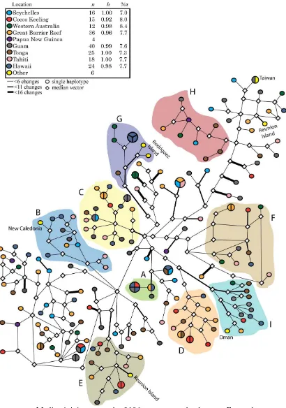
(42) basal to the other two clades. All three lineages were treated as three distinct nongeographic clades in AMOVA and for mismatch distributions. However, in many of our phylogenetic trees, clade 1 and clade 3 formed a single clade and are treated as such for some of our analyses. There were also three individuals that did not belong to any clade and were the basal taxa in our phylogenetic tree. It is likely that some homoplasy is present in the data (see Fig. 3.1 for example) but the underlying phylogenetic pattern is probably not destroyed by it.. Figure 3.1: (a) Rooted phylogram of 102 N. brevirostris mitochondrial control region sequences from BI. Posterior probability values indicate three clades in which there is no geographic pattern. Clade 2 also has bootstrap support from ML analysis (b) Median joining network of N. brevirostris haplotypes. Sample size (n), haplotype diversity (h) and nucleotide diversity (%π) are given. (c) Mismatch distribution of N. brevirostris haplotypes Fu and Li’s D and F tests of selective neutrality and Fu’s Fs value. Haplotypes marked with asterisks indicate sequences that are peculiarly arranged in the network and may be affected by homoplasy.. 29.

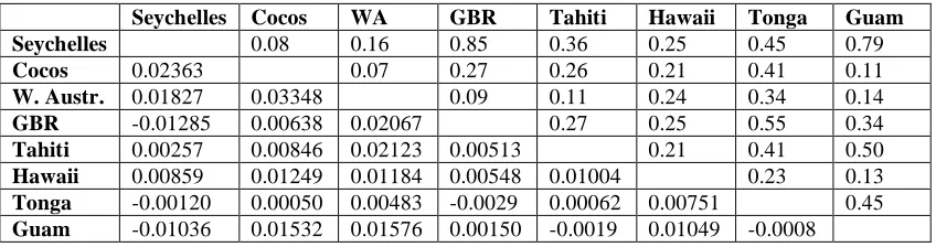
(43) 3.3.3 Population structure Pairwise Fst comparisons showed genetic differentiation between a subset of populations of N. brevirostris (Table 3.1). In particular, the Seychelles population was significantly different from Cocos Keeling, the GBR and French Polynesia. Pair wise Fst values increased gradually from west to east. Mantel test showed a significant and positive correlation between pairwise Fst values and pairwise geographic distance for N. brevirostris, indicating that isolation by distance is a factor in the gene flow of this species (r = 0.4757, p = 0.046). Log transformation of either variable did not significantly alter the outcome of the tests. All AMOVA fixation indices for this study showed no evidence of population structure for N. brevirostris between the Indian and Pacific Oceans (Φct = 0.008, p = 0.217) (Table 3.2). For this analysis, the boundary between ocean basins was experimentally placed in three different locations: (i) between eastern and western Australia, (ii) between western Australia and Christmas Island and (iii) between Christmas Island and Cocos Keeling. Moving the boundary in this way did not significantly change the AMOVA result. Hence, probably no barrier to gene flow exists between the Indian and Pacific Ocean basins. Likewise, there was no evidence of population structure for N. brevirostris between the east and west Indian Ocean, or western and central Pacific Ocean (Φct = 0.002, p = 0.453). However, when samples were segregated into the seven sampling locations (i.e. GBR, Seychelles, etc.), shallow population structure was detected for N. brevirostris (Φst = 0.0773, p = 0.006). In contrast to geographic tests of population structure, when the non-. 30.

(44) geographic clades of N. brevirostris were tested, deep population structure was found (Φst = 0.4996, p = 0.001). AMOVA analysis of N. vlamingii populations revealed shallow structure between sampling locations and ocean basins (Φst = 0.065, p < 0.05) and (Φst = 0.076, p < 0.05), respectively (Klanten et al. 2007). Unfortunately Klanten et al. (2007) did not perform AMOVA on the non-geographic clades of N. vlamingii therefore no comparison can be made with N. brevirostris.. Table 3.1: Population pairwise Fst for sampled N. brevirostris populations (below) and corresponding p values (above). Significant values appear in bold. Only the Seychelles population showed structure with any other population. Structure becomes stronger as the distance grows greater suggesting that remote populations are isolated by distance. S Seychelles. CK. CI. WA. GBR. SI. FP. 0.036. 0.441. 0.189. 0.018. 0.207. 0.000. 0.549. 0.360. 0.801. 0.846. 0.117. 0.585. 0.270. 0.531. 0.144. 0.162. 0.459. 0.702. 0.621. 0.072. Cocos. 0.042. Christmas. -0.008. -0.019. W. Australia. 0.063. -0.003. -0.034. GBR. 0.074. -0.021. 0.012. 0.023. Solomon Is.. 0.019. -0.043. -0.024. -0.023. -0.033. French Poly.. 0.162. 0.059. 0.042. -0.044. 0.068. 0.108 0.071. Table 3.2 AMOVA fixation indices (Φst) for N. brevirostris, percentage of genetic variation (%) and accompanying p values for four different comparisons: Overall (seven locations Seychelles-French Polynesia), Indian Ocean vs. Pacific Ocean, West Indian vs. East Indian+West Pacific vs. Central Pacific and clade vs. clade. Comparison. Fixation index. %. p. Overall AMOVA Indian Ocean vs. Pacific Ocean. Φst = 0.0773 Φst = 0.022 Φsc = 0.021 Φct = 0.008 Φst = 0.026 Φsc = 0.024 Φct = 0.002 Φst = 0.499. 2.63 97.01 2.11 0.88 97.3 2.46 0.22 50.4. p = 0.006 p = 0.081 p = 0.128 p = 0.217 p = 0.083 p = 0.122 p = 0.453 p = 0.001. West Indian vs. East Indian+West Pacific vs. Central Pacific Clade vs. Clade. 31.

(45) 3.3.4 Demographic Expansion Unlike N. vlamingii, the mismatch distribution of the N. brevirostris data set was bimodal (Fig. 3.1) and had a reported τ value of 25.5 with upper and lower bounds of 10.9 and 35.3 respectively. Using the methodology of Klanten et al. (2007), N. brevirostris mean expansion time was 11.1 MY, compared to N. vlamingii, which had a mean expansion time of 8.1 MY. Mean expansion times for the clades of N. brevirostris ranged between 2 and 5 million years ago (Figure 3.2) and are comparably dated with the clades of N. vlamingii. Fu & Li’s tests were not significant indicating that our marker is not under selection. Fu’s Fs was significantly negative (Fs=-24.00, p= 0.001). Globally, N. brevirostris is probably an expanding population rather than one that has remained stable over prolonged periods. Comparisons of θ0 and θ1 are suggestive of long-term population growth for this species as they were for N. vlamingii. Clade specific mismatch distributions of N. brevirostris (Fig. 3.2) revealed that clades one and three have unimodal mismatch distributions, suggestive of expansion, while clade two has an independently bimodal mismatch distribution and may not have evolved under the same conditions as the other clades. Fu’s Fs values are significantly negative for all clades. Fu & Li’s tests are not significant for clades one and two but for clade three they were significant, suggesting that there may be background selection acting on this clade alone. A combined clade 1 and 3 revealed a unimodal mismatch distribution and a significantly negative Fu’s Fs value (Fig. 3.2). Fu & Li’s tests of selective neutrality differed for this arrangement: Fu & Li’s D test was not significant, while Fu & Li’s F test was significant. According to Fu & Li (1993), F is a more sensitive test than D, therefore, we must assume a selection signal here. Nevertheless, combining clades 1. 32.

(46) and 3 appears only to have diluted the strong selection signal of clade 3 and may suggest that clades 1 and 3 are independent lineages that differ characteristically.. Figure 3.2: Clade Specific mismatch distributions with accompanying genetic diversity indices, neutrality tests and historical demographic values: τ, θ 0,θ1, which are respectively the time since expansion measured as 1/(2u) generations (see methods), effective female population size (Nef) at the time of expansion and Nef of the current population. Fu and Li’s D and F test assumptions of the neutrality of the genetic marker, while Fu’s Fs gives an indication of population expansion.. 33.

(47) 3.4 Discussion 3.4.1 Congruence with Naso vlamingii The broad-scale phylogeography of N. brevirostris is generally congruent with that reported for N. vlamingii by Klanten et al. (2007). N. brevirostris exhibits: 1) high genetic diversity in the mitochondrial control region, 2) a lack of spatial population partitions at a large spatial scales, 3) non-geographic clades that appear to be analogous with those found in N. vlamingii. The presence of non-geographic clades in a second Naso species suggests that these are not stochastic patterns but residual population structures. Considering that the expansion ages of clades from both species are comparable, it seems unlikely that the similarities between the two data sets could be explained by chance alone. However, it should be noted that these dates are heuristic estimations and not precise ages.. 3.4.2 Spatial patterns Haplotypes shared among sampled areas in the N. brevirostris data compellingly argue that distant locations are exchanging genes and that the minimal population structure is not due to inflated genetic variation. Some of these haplotypes are shared between Indian and Pacific populations, suggesting that inter-oceanic gene flow occurs in this species. However, isolation-by-distance was significant in N. brevirostris implying that dispersal in this species is limited and that distant populations exchange genes in a stepping-stone fashion. Overall AMOVA fixation indices showed no population structure on the largest geographic scales but on the smaller scale of our sampling locations (i.e. GBR, Solomon Islands, French Polynesia) shallow, yet significant, population structure was detected (Table 3.2). Population structure on a small scale but not on a. 34.

(48) large scale can be due to a scaling effect. When populations are classed by ocean basin, the ocean-wide population automatically has a much larger within-population diversity and a genetic signature that is more vague. Large conglomerate groups of populations, therefore, may appear to be highly connected but this does not mean that migration rates to each individual population are high (Wakeley & Aliacar 2001). Also, it is thought that only a small amount of gene flow is necessary to genetically homogenize populations (Slatkin 1987). Thus, migration between Indian and Pacific Ocean populations need not be high in order to produce the patterns observed in N. brevirostris. Nevertheless, because many reef organisms do show population structure across the IPB, N. brevirostris probably experiences more gene flow than these. We know that N. brevirostris is an impressive disperser because it has been reported vagrantly from the Galapagos islands (Randall 2002) nearly 5,500 km from the closest permanent populations in the central Pacific. The dispersal ability of this species appears to homogenize genetic populations between the Indian and Pacific Ocean basins across a potent biogeographic barrier. But the overall phylogeographic picture indicates that long-distance dispersal is a small percentage of the total gene flow. In reality, this species may employ several dispersal strategies on multiple spatial scales, as has been suggested for other reef fishes (Planes et al. 2009).. 3.4.3 Non-geographic clades The mismatch distribution of the entire N. brevirostris data set was distinctly bimodal (Fig. 3.1). Bimodal mismatch distributions are commonly observed in small terrestrial vertebrates such as rodents (Miller et al. 2006; Mora et al. 2007) and lizards (Strasburg et al. 2007), with limited dispersal ability. In these cases, bimodal. 35.

No results found