Finding exoplanets around eclipsing binaries: a feasibility study using Mt Kent & Moore Observatories

(1)

UNIVERSITY OF SOUTHERN QUEENSLAND

Finding Exoplanets Around

Eclipsing Binaries: A Feasibility Study Using

Mt Kent & Moore Observatories

(2)

(3)

Abstract:

The project aims to test the feasibility of using Mt Kent and Moore Observatories to find exoplanets in orbit around eclipsing binary stars. For these stars the timing of eclipse

variations caused by an orbiting planet is something suited to small telescopes as it relies on timing precision that can be readily obtained. In this project some test data for the eclipsing binaries V775 Centaurus and LT Herculis have been obtained using 0.5m aperture

telescopes at Mt Kent (Queensland) and Moore (Kentucky), and the data reduced and analysed to produce light curves and times of eclipse minima, in a very limited search for new planets. Although no evidence for a planet was found from the limited dataset

(5)

1. Introduction:

The search for exoplanets in orbit around distant stars has been a major focus of astronomy for many years, with more planets being discovered every month (websites like

exoplanets.org and planetquest.jpl.nasa.gov provide great examples). But these searches have previously focused on single star systems or those in widely separated binary systems. In order to provide a more complete census of the planets in our Galaxy it is necessary to search for planets in orbit around close binary star systems. This paper will focus on eclipsing binaries, binaries whose orbital inclination to us make each star periodically eclipse each other. The reasoning for this is that the significant decrease in luminosity during the eclipses can provides us with a great deal of information that can be readily modelled, of particular interest is variations in eclipse periods which can indicate the existence of additional orbital bodies in the system – notably planets.

This paper will explore a methodology that complements more traditional planet search techniques, and allows for the discovery of even low-mass exoplanets around binary stars. The method investigated here is a variant of the Transit Timing Variation (TTV) technique that is specially designed for eclipsing binaries, which allows for small aperture telescopes to be used. This project will test the viability of using the Mt Kent Observatory in

(6)

1.1. Exoplanets and Planetary Categories:

The discovery of exoplanets has given astronomers a great insight into planetary formation and the evolution of planetary systems over time. One of the reason that exoplanets are of such interest to astronomers is that in observing them we are able to expand our knowledge about how planets are formed, evolve and even migrate after formation. We can also learn a great deal about the effects stars have on their orbiting planets and how planets may

influence their host stars .

To date there are four categories of planets that have been observed, both in our Solar System and in other planetary systems. Below is a very brief outline of each type and how they are theorised to be formed:

1.1.1. Terrestrial Planets:

Terrestrial planets are simply defined as Earth-like, rocky planets and are usually of a smaller mass and radius then their gaseous cousins, but a higher density. These planets are formed closer to their host stars from the collision planetesimals and other bodies cotaining heavy elements. With our current models of planetary and stellar formation terrestrial planets can only form in the inner zones of the stellar planetary system (Bennett et al 2007).

1.1.2. Jovian Planets:

Jovian planets are the opposite to terrestrial planets, they are defined as large gaseous

(7)

system. They are formed through the accumulation of gas, dust and icy

particles/planetesimals, which can only occur at a significant distance from the host star (Bennett et al 2007). This is one of the reasons why we see a clear division and segregation between terrestrial and Jovian planets in our solar system.

1.1.3. Hot Jupiters and Super Earths:

Hot Jupiters and Super Earths are considered to be abnormalities in planetary systems but an abnormality that seems occurs frequently. Hot Jupiters are Jovian exoplanets that are found in close proximity to their host star, as close as 0.1 AU. As previously discussed Jovian planets should be able to form in such close orbits; this infers that either there is an error in our current model of planetary and stellar formation or some commonly occurring event has caused these outlying exoplanets to migrate into extremely close orbits.

Super Earths on the other hand are simply terrestrial planets that are significantly larger then was previously thought possible. These planets have all been found in close orbits to their host stars, but whether this is a characteristic of Super Earths, a feature caused by our limited search methods or simply a development that has not occurred locally is currently unknown.

1.2. Exoplanet Search Techniques:

(8)

method is radial velocity with less common methods being astrometry, pulsar timing and gravitational microlensing. Of the direct detection methods currently used the most popular technique is transit detections with direct imaging and coronagraphy being significantly less popular due to large limitations they incur but they are still important tool in exoplanet searches.

1.2.1. Astrometry:

Finding exoplanets via astrometry requires taking very precise measurements of a star's position over long periods of time and analysing any change in its position in the sky (Carroll & Ostlie 2007). The reasoning behind this technique is that a stellar system does not orbit around the host star but around the centre of mass of the system, due to the massive nature of stars the centre of gravity is usually close to the centre of host star. This results in the star orbiting around a point close to itself (or frequently, inside itself) causing a

'wobbling' effect. By calculating the mass and spectral type of the star it is possible to

ascertain the required mass and orbital radius a second celestial body that would be required to produce the variations in the host star's position. This particular technique is one of the oldest used in the field of exoplanet searches but at this time there has been no confirmed exoplanet discoveries using this method.

1.2.2. Radial Velocity:

(9)

used to describe the change in pitch of sound waves but same theory applies to

electromagnetic waves. This results in the compressed waves from an approaching star having a smaller wavelengths therefore reaching the receiver as slightly shifted into the blue end of the spectrum (blueshifted) while the expanded waves from a receding source have larger wavelengths resulting in the light reaching the receiver as shifted further into the red end spectrum (redshifted).

If the target star has another celestial body(s) orbiting itself and the planetary disc is

approximately parallel to our line of sight, the star will go through regular shifts in spectrum colour as its light changes from being blueshifted to redshifted (Cummings 2004). This is caused by the star orbiting the centre of mass of the system resulting in the previously mentioned 'wobbling' effect. This data can be used to calculate the orbital period of the star which is further used to calculate the minimum mass and nature of the planets in orbit around it. Unfortunately this method is only practical for finding massive exoplanets in close orbits to their host star.

1.2.3. Pulsar Timing:

Pulsars are the remnants of massive stars that have undergone supernovae and have become dense neutron stars. These stars release consistent, periodic bursts of electromagnetic

(10)

planetary system in orbit around it. This deviation in pulses allows for the calculation of the period and mass of the stellar and planetary bodies involved in the system. While this method is similar to the radial velocity technique it is far more accurate.

The major downside to this technique is that any planetary body in orbit around a pulsar will have suffered the effects of the preceding supernova. This means that the exoplanets in question will be vastly difference to any planetary body that we are familiar with.

Unfortunately this renders these planets less useful in furthering our understanding of the birth and mechanics of planetary systems but none the less makes they are an interesting celestial body to study (The Planetary Society 2005).

1.2.4. Gravitational Microlensing:

It was long theorised by Einstein that gravity warps the fabric of space-time, this can result in light being affected by large masses as the photons are refracted by the curvature of space-time. The gravitational microlensing method of detecting exoplanets uses this basic theory by using unknown exoplanets as gravitational lenses which will refract the light around them in much the same way as a convex lens (The Planetary Society 2005). The microlensing technique requires searching for stars or other luminous celestial bodies that undergone a rapid intensification in brightness, a sudden change in position or experience a twinning effect. These are key signs that there is a dark body (most likely a previously unknown exoplanet) between the receiver and the source.

(11)

previously located. The common twinning effect is cause by the same bending of light but with the light being refracted around both sides of the body resulting in the optical illusion of the light source appearing as two identical light sources some small distance apart (Bennett et al 2007).

This main advantage to this technique is that it can easily detect planets that are a great distance away from their host star but at the same time this method is difficult to use as the alignments are rare events and will only last for a few days or weeks and due to the

distances between the host star and the exoplanets it is problematic to try and preform follow-up observations.

1.2.5. Direct Imaging:

(12)

high surface temperature so that the it strongly emits in the infrared section of the spectrum.

1.2.6. Coronagraphy:

This method of detection is very similar to direct imaging but includes the use of a coronagraph. A coronagraph is type of telescope that uses a disc to block out all but the coronasphere of the target star so that the majority of the star light is blocked allowing the viewing of orbiting exoplanets. Unfortunately this proves to be more difficult in practice as the star light will diffract around the blocking disc and causing diffraction patterns making it difficult to gain useful data without either correcting for the diffraction or controlling the diffraction so that the patterns do not directly interfere with position of the exoplanet is (Sivaramakrishnan & Oppenheimer 2006). Thankfully this isn't too hard to do and there has been proposals for different shaped discs so that the diffraction can be easily kept away from key areas of the CCD chips on the coronagraphs. Again this method is mostly used as a technique to visually confirm the existence of previously detected exoplanets.

1.2.7. Transit Detection:

(13)

of the starlight that falls on it. This reflection results in the target star having a fractionally higher photon count then it would on its own so when the exoplanet passes behind the star the total luminosity will decrease (Gillion 2005).

The results from transit detection can give us very important information about the planetary radius, orbital radius and the rotational period of exoplanet. When this data is combined with secondary radial velocity data to confirm the rational period and the mass, the density of the target exoplanet can be ascertained. This allows for the planet to be classified as either a terrestrial or Jovian planet and allows an insight into the possible compositions of the target exoplanet.

One of the interesting abilities of transit detection is the ability to compare the change in absorption lines of the host stars spectrum in relation to the times where a planet is transiting its host star. There should be a constant and periodic change in the absorption lines that coincides with the transiting of the planet as a result of the atmosphere absorbing and re-emitting some of the starlight. This change in spectrum allows us to decipher the chemical composition of the exoplanet's atmosphere (Charbonneau et al 2002).

(14)

1.3. Transit Timing Variations (TTV):

Transit timing variation is a technique based on studying and analysing the transit periods for any anomalies that occur, usually in the length of time between each individual transit. These delays or advancements are produced by gravitational interactions between the observed transiting planet and an unknown planet(s). With the use of modified Lagrange and gravity equations it is possible to calculate the mass and orbital radius of the secondary planet(s) (Holman J. et al 2005).

The major advantage of transit timing variation technique is that it is able to detect planets up to one-tenth the mass of Earth, something that other technique can not accurately and reliably achieve. The use of transit timing variations also presents itself as a way to

circumvent one of that major problems that have existed in all forms of exoplanet hunting, in that the observation time needs to equal a multiple of the orbital period of the exoplanet in order to obtain accurate and useful data, this makes trying to find exoplanets far away from their host star both cost and time intensive. But with the TTV method the periods of planets with large orbital radii can be easily extrapolated from shorter period exoplanets in the same system (Nesvorny & Morbidelli 2008).

(15)

away or freezing.

1.4. Advantages of Transit Timing Variations:

There are many advantages the Transit Timing Variations (TTV) method has over it's earlier brethren. One of the major restriction of both Radial Velocity methods and Transit methods is that they are observing an event that is based around the orbital period of the exoplanet, this means that in cases of more distance exoplanets the amount of time that a star must be continuously observed rises from hours and days to months and years. Given the that stars are not observable for the entirety of the year, that telescope undergo maintenance and suffer faults as well as general bad weather it quickly becomes impractical for these methods to search for more distant exoplanets. Unlike both radial velocity methods and transit methods TTV is not restricted by close orbiting bodies as the method is searching for the perturbation effects of more distant bodies on that for a closer one rather then the direct pull or transit, this means that rather then having to have a base observation time anywhere between months and hundreds of years we only have base observation time of a few weeks.

1.5. Eclipsing Binaries:

Binaries are defined as stellar systems which contain two stars in close orbit of each other, therefore eclipsing binaries are defined as binary systems where the orbital plane of the two stars is parallel to the observer's line of sight. This means that as the stars orbit each other their combined magnitude will appear to periodically change as the stars move

in-front/behind one another. Of all the stars in the night sky binary stars make up

(16)

[image:16.595.73.541.94.305.2]

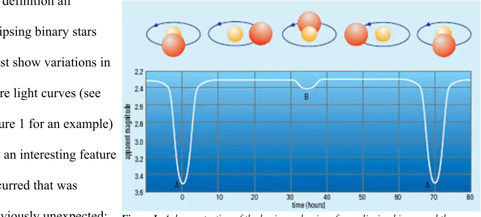
By definition all eclipsing binary stars must show variations in there light curves (see figure 1 for an example) but an interesting feature occurred that was

previously unexpected;

there were variations in the periods of the eclipses, not only that but this variations where occurring with a cyclical nature. For many years it was thought that this phenomenon was cause by one of two things: either magnetic activity occuring between the two stars or the gravitational effects of additional, darker bodies. In 2010 Lian and Qian published a paper on a survey they had preformed showing that these eclipse timing variations where still apparent in late type stars (with demonstrated little magnetic activity), this strengthening the concept that the majority (if not all) of observed eclipse timing variation is caused by

additional objects in the system, most likely an exoplanet.

Unfortunately detecting dark objects around binary stars has historically proven difficult because methods such as radial velocity and transit detect are ill suited to the task. The main reasons being that the Doppler shift change caused exoplanets is significantly smaller than the Doppler shift changes caused by the binaries orbiting themselves, this results in any possible planetary data being drowned out by the larger shifts in the host stars. A similar

(17)

(18)

2. Methodology:

2.1. Finding Exoplanets Around Eclipsing Binaries.

As discussed above the current methods of radial velocity and transit detection are ill-suited for the detection of exoplanets around eclipsing binaries, this is where a variation on the Transit Timing Variation method can be used to great effect.

(19)

By analysing this simplified planetary system we can calculate the mass and orbital radius of the exoplanet in question by using the equations in the following section. The only downside to this method is that unlike exoplanets transit TTV methodology, the base time can be much larger depending on the system.

2.2. The Mathematics.

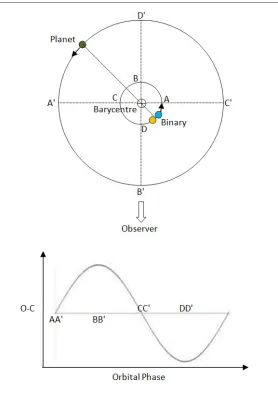
As previously discussed, an eclipsing binary system with one or more orbiting exoplanets will result in all the involved bodies orbiting around the barycentre as the binaries orbit each other, an example of such as system

can be seen below in figure 2. If the observer lies parallel to the plane of orbit (as depicted in the figure 2) there will be a significant variation in the distance between the eclipsing binaries and observer which changes over time. This change is distance will be detectable by a periodic variation in the timing of the eclipses. This

[image:19.595.260.538.301.695.2]

variance will follow a sinusoidal pattern with the latest delay occurring when the binary is at position B and the earliest eclipses occurring when the binaries are at point D (Tom

(20)

Richards 2011).

By plotting out this variation over time as an O-C diagram it possible to begin to learn a lot about the system. The amplitude of the sinusoidal pattern will correspond to the orbital radius of the binary from the barycentre in the direction of the observer (for example Ab= 0 at positions A and C). This amplitude will be equal to Ab/c, where Ab is the orbital radius of the binary from the barycentre and c is the speed of light.

By extension the amount of time delay between eclipses can be calculated as a ratio involved mass, speed and distance from the barycentre. The equation used for this time delay in the eclipses is:

t=ApMp

c Mb

Where Ap is the distance of the exoplanet from the barycentre in the direction of the

observer (Ap= 0 at A' and C'), Mp is the mass of the planet and Mb is the mass of the binary.

The next step is to calculate the period of the exoplanet, this is done by using Newton's modification of Kepler's Law. With is the period of exoplanet can be calculated by:

P2

=4p

2

AbAp

3

GM_bM_p

(21)

2.3. Software and Data Reduction

Most of this projects' data reduction and analysis was preformed by the AstroImageJ 2.0.0 software courtesy of Karen Collins. AstroImageJ is a modification of the ImageJ software released in 1997 by the National Institute of Health, the program was originally use as an open source imaging program to be used primarily for medical imaging but since then it has found popularity in other fields such as biology and astronomy. The AstroImageJ software modifies the original through a series of Java plugins and macros designed to allow for a number of astronomical operations to be preformed.

During the project the AstroImageJ software was used to preform data reduction on the images. This was accomplished by first averaging all of the dark images collected on a given night creating a master dark image, the same process is then completed with all of the bias images collected to create a master bias image. These master dark/bias images are used as way to remove any corruption from the data caused by instrument signature such as variation in pixel sensitivity, background noise and defective pixels or “hot pixels”. The master dark/bias images are then subtracted from all of the images collected on the night of observation. After this a master flat field image was created by once again averaging all of the collected flat fields. The master flat field is then divided from the observed data to remove an gradient error resulting from telescope and CCD impurities (dust particles, etc) as well as any gradient error caused by uneven sky illumination.

(22)

number (4-5) stable comparison stars. This process analyses the flux of each selected star in the frame and compares it to the others. This is designed to assure the any variations in the flux of the target star are a result of the a stellar effect and not simply a observation error. Once all of the data has been collected, the relative flux of the target star is plotted versus the flux of the comparison stars, this creates the light curve plots seen in figures 4,5 and 7-10.

2.4. Observatories and Instruments

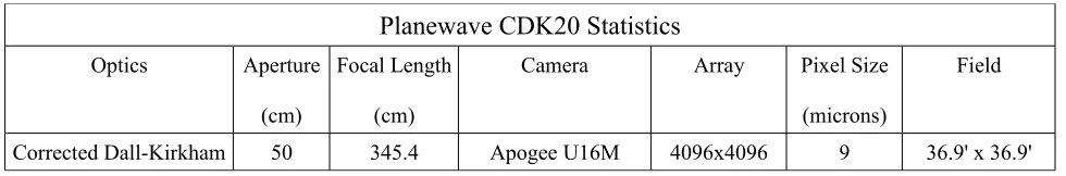
This project took photometric data on two eclipsing binaries; V775 Cen and LT Her. All of the V775 Cen data was taken using the Planewave CDK20 telescope at the MT Kent

Observatory in Toowoomba, Australia. The telescope is a 0.508m Corrected Dall-Kirkham with a Apogee U16M CCD camera granting a 36.9'x36.9' field of view. A UBVRI filter wheel was used with all images taken using the V filter with an exposure time of 10 seconds.

(23)

Planewave CDK20 Statistics

Optics Aperture

(cm)

Focal Length

(cm)

Camera Array Pixel Size

(microns)

Field

[image:23.595.54.544.55.136.2]

Corrected Dall-Kirkham 50 345.4 Apogee U16M 4096x4096 9 36.9' x 36.9'

Table 1: The specifications of the Planewave CDK20 used by both the Mt Kent Observatory and the Moore Observatory to collect data on V775 Cen and LT Her.

The data reduction was preformed using a variation of the ImageJ software called

(24)

3. Results:

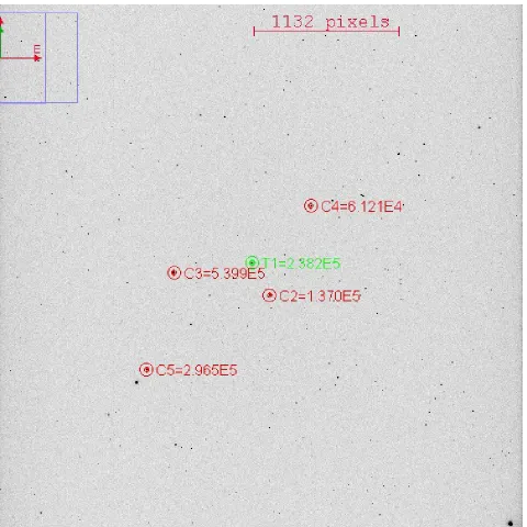
Two eclipses of V775 Cen were observ ed on the 12th_{of May (secondary minima) and the}

13th_{of May (primary minima) using the Mt Kent Observatory. The images of V775 Cen}

[image:24.595.61.541.215.695.2]

were taken in using a V filter with 10 second exposures over a period of 2-3 hours. The field of view can be seen in figure 3.

(25)

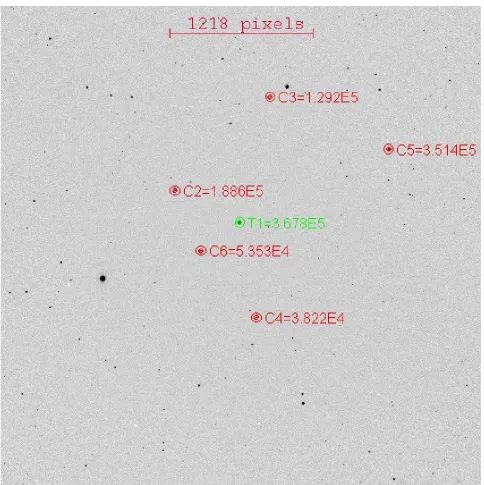
Four primary eclipses were observed for LT Her by John Kielkopf on the 17th_{, 18}th_{and 30}th

of May as well as on the 9th_{of June. All images were taken using an R filter with 50 sec}

exposure times. The image field can be seen in figure 6. All target stars are highlighted by the green apertures with the check stars highlighted by the red apertures.

All of the data was processed by first creating master dark and master bias images by taking the average of multiple such images. A master flat field was created by subtracting the master darks and biases from all flat field images and then taking there average. All of the taken images where then processed by subtracting the darks and biases from the raw data and dividing the result by the master flat field. Once the basic image processing was completed, a multi-aperture and alignment function was run over the images to gain a reading and to plot the target star's relative flux over time. All of the data processing, photometry and plotting was preformed by the AstroImageJ 2.0.0. software, which was provided by Karen Collins.

(26)

Observed time of eclipse (HJD) Calculated time of eclipse (HJD) O-C (d) Error (d)

V775 Cen 2456060.07890 2456060.08200 -0.00310 ±0.00010 2456061.07450 2456061.07746 -0.00296 ±0.00005

LT Her

- 2456065.60468 -

-2456066.68809 2456066.68871 -0.00062 ±0.00003 2456078.54780 2456078.61308 -0.06528 ±0.00003

- 2456088.36937 -

-Table 2: A table of all the data taken on each night. There was a timing error on the 17/05/12 and 09/06/12 which resulted in no light curve being recorded.

All of the minima times have been uploaded in to the MT Suhora Astronomical Observatory data base of eclipsing binaries. The data collected by this project is still awaiting verification by the MT Suhora Astronomical Observatory but the O-C diagrams for the previously

[image:26.595.58.540.55.178.2]

(27)

[image:27.595.71.529.76.537.2]

(28)

[image:28.595.72.531.74.536.2]

(29)

[image:29.595.57.541.57.542.2]

(30)

[image:30.595.68.530.73.537.2]

(31)

[image:31.595.71.533.50.496.2]

(32)

[image:32.595.73.532.75.530.2]

(33)

[image:33.595.73.530.75.531.2]

(34)

[image:34.595.65.458.55.626.2]

Table 3: Previously collected data on V775 Cen with the a large portion of the O-C data missing due to a clerical error. Provided by www.as.up.krakow.pl.

Time (HJD) Error (d) Eclipse Type Detection

2416636.6790 - p

2418126.5670 - p

2418856.5820 - p

2419227.5540 - p

2420326.5480 - p

2424698.6290 - p

2425421.3450 - p

2427980.3450 - p

2428639.3600 - p

2428662.5750 - p

2428698.3970 - p

2428740.2500 - p

2429525.3060 - p

2432291.3610 - p

2432356.4110 - p

2432384.2890 - p

2433001.4830 - p

2438494.4470 - p

2438498.4500 - p

2438500.4400 - p

2438502.4380 - p

2438504.4380 - p

2438528.3350 - p

2438555.4590 - p

2438879.4030 - p

2438881.3760 - p

2439210.4860 - p

2439232.4170 - p

2439236.4580 - p

2439240.4120 - p

2440711.0190 - p

2440744.9000 - p

2441068.0000 - p

2441093.9660 - p

2441099.9410 - p

2441121.8490 - p

2441470.8760 - p

2441472.9020 - p

2451961.7670 - cc

2455294.5729 0.0002 cc

2455305.5253 0.0009 sec cc

V775 Cen Minima

[image:34.595.295.534.69.666.2]

pri pri pri pri pri pri pri pri pri pri pri pri pri pri pri pri pri pri pri pri pri pri pri pri pri pri pri pri pri pri pri pri pri pri pri pri pri pri pri pri

Table 4: Previously collected data on LT Her. Provided by www.as.up.krakow.pl.

LT Her Minima

Time (HJD) Error (d) Eclipse Type Detection

2430893.2180 - v

2430919.2280 - v

2431021.1360 - v

2431242.2610 - v

2440755.7594 - e

2441864.7403 - e

2445820.4560 - v

2447266.5049

-2447266.5091

-2447653.5136

-2447653.5150

-2448014.4990

-2448762.4734 0.0007 e

2449060.5783 0.0010 2449060.5842 0.0009 2449472.5069 0.0022 2449472.5105 0.0014 2449859.5156 0.0020

2451287.7312 0.0009 sec cc

2451308.8692 0.0007 cc

2451386.3533 0.0016 sec cc

2451386.9077 0.0026 cc

2451703.4593 0.0100 cc

2452426.5059 0.0011 cc

2453408.6264 0.0048 cc

2453589.6659 0.0006 cc

2453774.4927 0.0027 sec cc

2453775.0367 0.0008 cc

2454218.4095 0.0021 cc

2454235.7502 0.0005 cc

2454244.4224 0.0008 cc

2454261.7725 0.0003 cc

2454296.4520 0.0008 cc

2454555.5385 0.0003 cc

2454596.7338 0.0008 cc

2454608.1716 - sec cc

2454941.4588 0.0009 cc

2454945.7946 0.0001 cc

2454945.7970 0.0002 cc

2455340.3867 0.0011 cc

2455345.8105 0.0004 cc

2455353.3967 0.0025 cc

2455707.8793 0.0004 cc

2455752.3184 0.0001 cc

2455778.3450 0.0001 cc

(35)

[image:35.595.88.502.51.355.2] [image:35.595.88.514.413.711.2]

Figure 10: An O-C diagram of data taken of LT Her since 1904. The data that was taken has been uploaded on this

(36)

4. Discussion:

4.1. Light Curves and Minima:

The light curves of V775 Cen shown in figure 4 and figure 5 are typical of a binary system where one star is significantly brighter then it's companion, with the primary eclipse having a much larger impact on the luminosity as the cooler star blocks light from the brighter partner. The light curve from the 13th_{of May shows a clear primary eclipse with little to no}

noise or error and a deep decrease in magnitude. While the light curve taken from the 12th_of

May displays a much shallower light curve characteristic of a secondary eclipse. Due to the deeper drop in magnitude on the night of the 13th_{, the Minima software was able to}

determine a much more accurate minima time then on the shallower, secondary minima. For this reason primary minima are the most commonly used data points in eclipsing binaries research, with many telescopes and software unable to detect the very small decreases. One of the many interesting and promising results to come out the data taken at the MT Kent Observatory was the CDK20's ability to accurately detected the secondary minima on V775 Cen and for the exact minima time to be determined with only an error of ±0.0001.

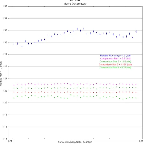
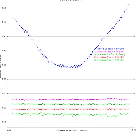
Some of the light curves produced from the LT Her data are not currently usable to obtain minima times as there was a time zone miscalculation on the nights of the 17th_{of May and}

9th_{of June. The miscalculation resulted in LT Her being observed 2 hours later then}

originally intended, there is still evidence of the eclipses occurring in the slow rise and levelling off of the luminosity but the data is not usable for the project. There was also a calculation error for the timing on the night of the 30th_{of May which resulted in}

(37)

Despite the incomplete light curve on the 30th_{it was still possible to use the Minima}

software to obtain an exact minima, but I am unsure as to the exact accuracy of this measurement due to the heavy extrapolation involved.

4.2. Viability of the MT Kent Observatory and Future Research:

The confirmation of exoplanets via the eclipsing time variation methodology was always beyond the scope of this project due to the large amount of observation time required. However this was not the main focus. The most important aspect of the results was that the project successfully demonstrated the viability of the MT Kent and Moore Observatories to detect exoplanets around of eclipsing binaries using a variation of the TTV technique. All eclipses, primary and secondary, were easily detected with their corresponding light curves containing little error. The exact time of each minima is easily and accurately determined, this allows for the most important aspect of TTV exoplanet searches to be to obtained; precise observed minus calculated (O-C) data.

(38)

4.3. Observation Conditions and Potential Errors:

On both nights used to take the V775 Cen data the sky was clear with the exception of some potential light, scattered cloud on the night of the 12th_{of May from 21:00 until 23:00. From}

the plot in figure 4 it would appear that if there was any cloud that it had little to no effect on the CDK20's visibility. The night of the 13th_{was clear of all cloud but it was noticed that}

the dome had begun to obscure the eastern edge of the field of view of the scope at 01:06, this was quickly rectified and the data taken around this time did not appear to contain any corruption or irregularities caused by this event. The wind speed was and sky temperature were low on both nights of observations.

The weather conditions in Louisville on the four nights that the data on LT Her was obtained were clear with no cloud cover being recorded and no errors occurring with the telescope or any of the software. The wind speed and sky temperature at the Moore Observatory were also low on all nights

(39)

5. Summary:

The project aimed to test the MT Kent and Moore Observatories' ability to detect exoplanets around eclipsing binaries. This was done by using both of the observatories' CDK20

telescopes to analyse the timing of the binaries eclipses to test for variations in the events which would be caused by orbiting exoplanets. Data was taken on two stars over several nights from both the MT Kent and Moore Observatories, which detected significant decreases in magnitude. In conclusion it was found that both observatories are well

equipped to preform this kind of research and there are plans to continue this research in to the future.

Acknowledgements:

(40)

References:

1. Ostlie, DA & Carroll, BW, 2007, An Introduction to Modern Stellar Astrophysics, 2nd edn, Pearson, San Francisco.

2. Bennett, J, Donahue, M, Schneider, N & Voit, M, 2007, The Cosmic Perspective, 4h edn, Pearson, San Francisco.

3. Holman, MJ & Murray, NW 2005, The Use of Transit Timing to Detect Terrestrial-Mass Extrasolar Planets, Science, vol 307, pp 1288-1291

4. Nesvorny D & Morbidelli, A 2008, Mass and Orbit Determination From Transit Timing Variations of Exoplanets, The Astrophysical Journal, vol 688, pp 636-646

5. Cummings, A 2004, Detectability of Extrasolar Planets in Radial Velocity Surveys, MNRAS, vol 354, 1165-1176

6. The Planetary Society, 2005, 4/10/2011, http://planetary.org/exoplanets/howwefind.php 7. Planet Quest, 2011, NASA, 4/9/2011, http://planetquest.jpl.nasa.gov/index.cfm

8. Sivaramakrishnan, A & Oppenheimer, BR 2006, Astrometry and Photometry with Coronagraphs, The Astrophysical Journal, vol 647, 620-629

9. Oppenheimer, BR 2003, Imaging Exoplanets, The Future of Small Telescopes, vol 3, 157-174

10. Charbonneau, D, Brown, TM, Noyes, RW & Gilliland, RL 2002, Detection of an Extrasolar Planet Atmosphere, The Astrophysical Journal, vol 568, 377-384

11. Gillion, M, Courbin, F, Magain, P & Borguet, B 2005, On the Potential of Extrasolar Planet Transit Surveys, Astronomy & Astrophysics, No 3030

(41)

13. Tom Richards, 2011, Variable Stars South,16/8/2011,

http://www.variablestarssouth.org/index.php/research-projects/spades

14. Liao, WP & Qian, SB 2010, The most plausible explanation of the cyclical changes in close binaries: the case of the RS Cvn-type binary WW Dra, Astronomy Society, No 000.

15. Prsa, A, Batalha, N, Slawson, RW, Laurance, RD, Welsh, WF, Orosz, JA, Seager, S, Rucker, M, Mjaseth, K, Engle, SG, Conroy, K, Jenkins, J, Caldwell, D, Koch, D & Borucki, W 2011, Kelper Eclipsing Binary Stars. I. Catalog and Principal Characterizations of 1879 Eclipsing Binaries in the First Data Release, arXiv:1006.281v2 [astro-ph.SR]

(42)

Appendix A

Date: 12/5/12 Target: V775Cen

Camera temperature: -10C

Filter set: 1=U, 2=B, 3=V, 4=R, 5=I, 6=blank Finding target

20:20 V775Cen0001.fits 10s V Had to focus

V775Cen0002.fits “ “ Plate solved and referenced Moved to target (Scope is on west side of mount, high altitude)

V775Cen0003.fits “ “ Target identified in field centre at (2033,2058). 14081 counts

Note: Had to flip Y to match ref frame from Czech site

V775Cen0004.fits 20s V Some elongation in X 21:24 T=17C DP=6C 50%RH 1016.7hPa Wind speed=0km/hr V775Cen0005.fits 20s V

V775Cen0006.fits

V775Cen0007.fits 60s V 5 pixel streaks in X

V775Cen0008.fits " “ 3 pixel streaks in X:different!(Az166, Alt65) Reposition so scope on East of mount

V775Cen0010-11.fits 10s V Finding target

V775Cen0012.fits “ “ on target 25000 counts V775Cen0013.fits 20s V

23:02 T=17C DP=6C 48%RH 1016.0hPa Wind speed=0km/hr V775Cen0014.fits 10s V 15000 counts

V775Cen0015.fits “ “ ST -31.9

V775Cen0016-18.fits “ “ ST -31.7 19000-14000 V775Cen0021.fits “ “ ST -31.5 19000

V775Cen0024.fits “ “ ST -31.2

V775Cen0034-62.fits “ “ first of 10 frame multi exposure ST -32.0 possible light/scattered cloud cover moving across on the radar

V775Cen0063-116.fits 10s V Moon Rising ST -32.2 V775Cen00117.fits “ “ ST -32.8

V775Cen00164-173.fits 10s V Dark V775Cen00174.fits 2s V Flat

(43)

Date: 13/05/2012 Target: V775 Cen

Camera temperature: -10C

Filter set: 1=U, 2=B, 3=V, 4=R, 5=I, 6=blank

V775Cen0001-5.fits 10s V Used to solve telescope and find target telescope on east side of mount

21:57 T=9C DP=0C RH 55% 1019.0hpa wind 3km/hr Av 6km/hr ST -35.9C

22:03

V775Cen0006-15.fits 10s V Counts 22000-17600 22:13

V775Cen0016-25.fits “ “ Counts 18000-18000 ST -38.5 22:18

V775Cen0026-35.fits “ “ 22:27

V775Cen0036-45.fits “ “ ST -37.3

V775Cen0046-425.fits “ “

23:03 ST -37.1 23:19 ST -35.0C

23.49 T=8C DP=0C RH 60% 1 019.0hPa Wind 3km/hr Av 3km/hr ST -35.8C

00:00 ST -37.2C

00:07 T=*C DP=0C RH 59% 1018.8hPa wind 5km/hr Av 6km/hr ST -35.4C

00:28 ST -36.7C 00:42 ST -36.3C 01:00 ST -35.6C

01:06 Noticed scope ~1/3 obscured by

dome. Moon just rising.

01:30 T=7C DP=1C RH 62% 1018.8hPa wind 5km/hr Av 5km/hr ST -35.9C

(44)

(45)

Appendix B

V775Cen on the night of 12/5/2012 Julian Date:

+2400000 Flux of Target Star

Flux of Comparison Star 1

56060.043426 0.316047 0.153097 1.086799

56060.046065 0.315140 0.150852 1.089713

56060.048333 0.313195 0.152131 1.093471

56060.051933 0.312048 0.152212 1.088532

56060.055405 0.310420 0.153385 1.083529

56060.058067 0.309646 0.154158 1.081521

56060.060243 0.308201 0.152556 1.085969

56060.060938 0.307753 0.152252 1.087369

56060.061632 0.308211 0.152056 1.092216

56060.062222 0.307600 0.151384 1.088338

56060.063102 0.308960 0.153673 1.091389

56060.065833 0.306138 0.152293 1.087012

56060.066887 0.304565 0.151847 1.091458

56060.067315 0.307162 0.153082 1.086968

56060.067975 0.307314 0.153566 1.080800

56060.068958 0.307055 0.152984 1.082997

56060.069722 0.307092 0.153084 1.083646

56060.070394 0.307412 0.153245 1.080227

56060.071308 0.307838 0.152641 1.084524

56060.071736 0.306485 0.153593 1.086527

56060.072593 0.306173 0.153355 1.091325

56060.072951 0.306590 0.152972 1.089322

56060.073299 0.307248 0.153415 1.089276

56060.073657 0.305791 0.153548 1.082781

56060.074016 0.307016 0.153180 1.089732

56060.074375 0.306308 0.151989 1.087549

56060.074722 0.307328 0.152452 1.092290

56060.075081 0.305319 0.153432 1.087874

56060.075440 0.304630 0.153561 1.080254

56060.075799 0.306004 0.153968 1.084750

56060.076285 0.305543 0.153299 1.090715

56060.076644 0.306035 0.153835 1.084019

56060.077002 0.306428 0.153439 1.089262

56060.077361 0.306895 0.153367 1.082296

56060.077708 0.305089 0.153538 1.087156

56060.078067 0.305121 0.152535 1.088859

56060.078426 0.306145 0.153004 1.084739

56060.078785 0.304460 0.152571 1.092613

56060.079132 0.305254 0.153030 1.085263

(46)

56060.080347 0.305431 0.152920 1.087940

56060.080706 0.307334 0.153657 1.085049

56060.081065 0.306568 0.152740 1.080718

56060.081412 0.304662 0.153743 1.082412

56060.081771 0.305490 0.153599 1.086940

56060.082130 0.306018 0.153215 1.085437

56060.082488 0.306425 0.153090 1.087791

56060.082836 0.307465 0.153477 1.086264

56060.083194 0.307117 0.153283 1.084047

56060.083553 0.304547 0.153064 1.086777

56060.084155 0.306568 0.153320 1.079993

56060.084502 0.305325 0.152815 1.086321

56060.084861 0.306781 0.153689 1.074603

56060.085220 0.306059 0.152806 1.083551

56060.085579 0.305732 0.153317 1.085556

56060.085926 0.306770 0.153279 1.082326

56060.086285 0.306962 0.152576 1.079873

56060.086644 0.307028 0.152840 1.081163

56060.087002 0.307742 0.152953 1.084148

56060.087350 0.307049 0.152782 1.082475

56060.087743 0.305552 0.153186 1.086116

56060.088102 0.305905 0.153000 1.089377

56060.088461 0.307676 0.152836 1.088544

56060.088819 0.306518 0.153087 1.082215

56060.089167 0.306907 0.154035 1.083063

56060.089525 0.307974 0.153666 1.080478

56060.089884 0.308989 0.154160 1.087214

56060.090243 0.307200 0.153291 1.090563

56060.090590 0.306624 0.151786 1.083202

56060.090949 0.306726 0.153300 1.087392

56060.091574 0.309260 0.153096 1.083993

56060.091933 0.308885 0.153554 1.085657

56060.092280 0.308230 0.153439 1.087137

56060.092639 0.307709 0.153015 1.080747

56060.092998 0.306941 0.153638 1.082178

56060.093356 0.306676 0.152529 1.086788

56060.093704 0.308764 0.152359 1.087575

56060.094063 0.308177 0.153103 1.086219

56060.094421 0.308178 0.152821 1.084989

56060.094780 0.309256 0.153275 1.084688

56060.095174 0.307958 0.153772 1.089250

56060.095532 0.307400 0.153048 1.083670

56060.095891 0.308538 0.153732 1.083233

56060.096250 0.307677 0.154310 1.081173

(47)

56060.096956 0.308664 0.153175 1.084848

56060.097315 0.307576 0.152018 1.089153

56060.097674 0.309852 0.153341 1.088683

56060.098032 0.308680 0.153393 1.081852

56060.098391 0.309830 0.153433 1.084132

56060.098843 0.311228 0.153364 1.080999

56060.099201 0.308125 0.151846 1.088522

56060.099560 0.309573 0.153845 1.087294

56060.099919 0.308561 0.152895 1.087555

56060.100278 0.311259 0.152788 1.085203

56060.100625 0.309690 0.153785 1.081834

56060.100984 0.309893 0.151586 1.093428

56060.101343 0.308164 0.152414 1.085313

56060.101701 0.310675 0.152585 1.082253

56060.102060 0.310643 0.153182 1.089302

56060.102500 0.310020 0.153115 1.086651

56060.102859 0.310334 0.153114 1.089176

56060.103218 0.310168 0.153743 1.075910

56060.103576 0.312016 0.153690 1.082316

56060.103924 0.311176 0.153193 1.083820

56060.104282 0.309886 0.153620 1.083509

56060.104641 0.311082 0.154811 1.076805

56060.105000 0.310823 0.153794 1.081444

56060.105359 0.311768 0.152890 1.083309

56060.105706 0.310424 0.154132 1.078028

56060.106609 0.313061 0.153274 1.081435

56060.106968 0.312880 0.153701 1.081737

56060.107326 0.311588 0.154094 1.076744

56060.107674 0.311855 0.152732 1.085057

56060.108032 0.312619 0.153910 1.082330

56060.108391 0.312347 0.154068 1.085230

56060.108750 0.313785 0.154446 1.079590

56060.109109 0.312050 0.153384 1.078699

56060.109468 0.313390 0.153569 1.082898

56060.109815 0.313174 0.152193 1.079639

56060.113137 0.314521 0.153988 1.084731

56060.113495 0.314681 0.153450 1.080671

56060.113854 0.315712 0.154037 1.085578

56060.114201 0.315065 0.154022 1.078057

56060.114560 0.314761 0.153939 1.078933

56060.114919 0.316700 0.153351 1.076181

56060.115278 0.316113 0.154274 1.080724

56060.115637 0.315189 0.153945 1.078751

56060.115984 0.314907 0.153160 1.084752

(48)

56060.116736 0.314935 0.153802 1.083351

56060.117095 0.317208 0.154294 1.080258

56060.117454 0.315016 0.154767 1.074787

56060.117801 0.316686 0.153508 1.082991

56060.118160 0.318476 0.154630 1.080352

56060.118519 0.318332 0.153560 1.079148

56060.118877 0.318156 0.154684 1.075279

56060.119236 0.317307 0.153400 1.083190

56060.119595 0.318886 0.153384 1.078204

56060.119942 0.319067 0.154320 1.085485

56060.120718 0.318535 0.154895 1.075750

56060.121076 0.317338 0.154106 1.078437

56060.121435 0.318683 0.153250 1.077387

56060.121794 0.319436 0.154570 1.083442

56060.122141 0.320542 0.154232 1.080534

56060.122500 0.320416 0.154281 1.077146

56060.122859 0.317999 0.152754 1.085412

56060.123218 0.319936 0.154592 1.080726

56060.123576 0.319941 0.154211 1.073919

(49)

V775Cen on the night of 13/5/2012 Julian Date:

+2400000

Flux of Target Star Flux of Comparison Star 1

56061.001516 0.322520 0.154082 1.095276

56061.001875 0.321550 0.152878 1.091341

56061.002234 0.319974 0.152389 1.092466

56061.002581 0.318586 0.153164 1.096591

56061.002940 0.321628 0.152744 1.095447

56061.003299 0.319394 0.152813 1.091288

56061.003646 0.319519 0.152060 1.096570

56061.004005 0.319847 0.152284 1.095840

56061.004363 0.320387 0.153909 1.095603

56061.004722 0.321155 0.152728 1.088727

56061.008287 0.315463 0.154385 1.092643

56061.008646 0.315535 0.152417 1.094153

56061.009005 0.316401 0.152103 1.083586

56061.009363 0.313001 0.152663 1.100409

56061.009711 0.312710 0.153288 1.091454

56061.010069 0.312203 0.152301 1.095051

56061.010428 0.312901 0.152527 1.101716

56061.010775 0.312427 0.152742 1.098151

56061.011134 0.309638 0.152983 1.095823

56061.011493 0.310768 0.152562 1.092136

56061.012593 0.309110 0.152481 1.098787

56061.012940 0.309379 0.153148 1.094628

56061.013299 0.307873 0.153261 1.095766

56061.013657 0.307302 0.153587 1.089257

56061.014005 0.307750 0.151265 1.107513

56061.014363 0.307311 0.153544 1.084716

56061.014722 0.306629 0.153888 1.086953

56061.015081 0.305402 0.152706 1.086504

56061.015428 0.306340 0.153449 1.089793

56061.015787 0.305564 0.154045 1.088251

56061.019039 0.301722 0.154470 1.083770

56061.019398 0.297878 0.153586 1.088415

56061.019745 0.297816 0.153057 1.088880

56061.020104 0.296621 0.152828 1.097004

56061.020463 0.294967 0.152838 1.098324

56061.020810 0.296720 0.152043 1.094784

56061.021169 0.295147 0.153203 1.086798

56061.021528 0.294177 0.153667 1.091853

56061.021875 0.295399 0.152505 1.093081

56061.022234 0.292222 0.152700 1.092379

56061.023356 0.290292 0.153350 1.088778

(50)

56061.024063 0.288276 0.151977 1.100073

56061.024421 0.290479 0.153280 1.094242

56061.024780 0.287285 0.153135 1.094594

56061.025139 0.287620 0.152904 1.091808

56061.025486 0.285112 0.153735 1.094523

56061.025845 0.286617 0.152457 1.095267

56061.026204 0.283997 0.152739 1.090047

56061.026563 0.284552 0.154441 1.081691

56061.027569 0.281145 0.152148 1.097520

56061.027928 0.280867 0.152817 1.095325

56061.028287 0.279940 0.154265 1.085134

56061.028634 0.278940 0.153426 1.090783

56061.028993 0.277952 0.152329 1.092646

56061.029352 0.277656 0.152247 1.091694

56061.029711 0.277654 0.152706 1.092711

56061.030058 0.276963 0.153581 1.087061

56061.030417 0.275387 0.153020 1.096201

56061.030775 0.275118 0.152710 1.097409

56061.032384 0.271397 0.152798 1.095425

56061.032731 0.272056 0.153584 1.090268

56061.033090 0.270132 0.153689 1.093897

56061.033449 0.269438 0.153398 1.085732

56061.033808 0.269692 0.154062 1.090093

56061.034155 0.268886 0.153832 1.093647

56061.034514 0.269336 0.152836 1.091351

56061.034873 0.266590 0.153315 1.092890

56061.035220 0.266782 0.151776 1.094683

56061.035579 0.266841 0.154571 1.087207

56061.036898 0.261459 0.152398 1.086948

56061.037257 0.261040 0.153800 1.094308

56061.037604 0.260556 0.152972 1.092176

56061.037963 0.259948 0.153714 1.098286

56061.038322 0.259147 0.153421 1.087983

56061.038669 0.258030 0.152658 1.091432

56061.039028 0.257766 0.153718 1.091099

56061.039387 0.256849 0.154082 1.094705

56061.039745 0.254360 0.153307 1.094739

56061.040104 0.254487 0.153495 1.091248

56061.041597 0.249976 0.153081 1.094550

56061.041944 0.251501 0.154264 1.092299

56061.042303 0.249268 0.153403 1.093344

56061.042662 0.249730 0.153999 1.087532

56061.043021 0.248976 0.152861 1.089748

56061.043368 0.247248 0.153273 1.097103

(51)

56061.044086 0.245430 0.153099 1.089788

56061.044444 0.244064 0.153486 1.093533

56061.044792 0.244621 0.152250 1.091595

56061.045706 0.242163 0.153819 1.091654

56061.046065 0.240937 0.152926 1.089422

56061.046412 0.239011 0.152608 1.091192

56061.046771 0.238164 0.153893 1.091376

56061.047130 0.238550 0.153666 1.088356

56061.047488 0.237473 0.152611 1.095656

56061.047836 0.237040 0.153084 1.088182

56061.048194 0.235495 0.153346 1.083630

56061.048553 0.235113 0.152793 1.092361

56061.048912 0.234635 0.152902 1.093316

56061.049375 0.234679 0.153998 1.087225

56061.049734 0.232727 0.152858 1.093440

56061.050093 0.229938 0.153101 1.093230

56061.050440 0.230245 0.152652 1.090990

56061.050799 0.229606 0.153893 1.088506

56061.051157 0.229711 0.152797 1.094162

56061.051516 0.227365 0.153919 1.094587

56061.051863 0.228266 0.152923 1.094041

56061.052222 0.227005 0.152066 1.095296

56061.052581 0.225225 0.152459 1.090166

56061.053461 0.225925 0.153992 1.091460

56061.053808 0.223636 0.152234 1.086072

56061.054167 0.222594 0.152808 1.093028

56061.054525 0.221597 0.153233 1.086704

56061.054873 0.221407 0.153839 1.088829

56061.055231 0.220015 0.152387 1.092419

56061.055590 0.219961 0.153433 1.093629

56061.055949 0.219458 0.152505 1.101113

56061.056296 0.216484 0.152674 1.089624

56061.056655 0.216992 0.153155 1.095469

56061.057049 0.218292 0.153029 1.091267

56061.057407 0.214493 0.152890 1.084216

56061.057755 0.214345 0.153620 1.095232

56061.058113 0.214835 0.153271 1.093941

56061.058472 0.213763 0.152917 1.095389

56061.058819 0.213314 0.154373 1.089806

56061.059178 0.213262 0.153269 1.101129

56061.059537 0.211076 0.152796 1.095825

56061.059896 0.211500 0.151599 1.095241

56061.060243 0.210819 0.152516 1.098580

56061.060660 0.210858 0.151429 1.100705

(52)

56061.061377 0.209712 0.153398 1.087622

56061.061725 0.208605 0.154696 1.088697

56061.062083 0.207845 0.151313 1.094802

56061.062442 0.207034 0.153089 1.101107

56061.062789 0.207026 0.154037 1.082204

56061.063148 0.207497 0.152748 1.083168

56061.063507 0.207210 0.153443 1.090482

56061.063866 0.205495 0.153690 1.095429

56061.064248 0.207290 0.153436 1.078375

56061.064606 0.203853 0.151182 1.105669

56061.064965 0.202873 0.153957 1.091339

56061.065324 0.203307 0.152623 1.091571

56061.065671 0.201491 0.155254 1.084559

56061.066030 0.200770 0.152970 1.084947

56061.066389 0.204166 0.154379 1.090025

56061.066736 0.201370 0.151696 1.097270

56061.067095 0.201971 0.153735 1.093775

56061.067454 0.201203 0.152542 1.084028

56061.067963 0.201483 0.152634 1.094175

56061.068310 0.202465 0.154133 1.090059

56061.068669 0.199556 0.153328 1.087469

56061.069028 0.199555 0.153114 1.101152

56061.069375 0.200323 0.153319 1.093863

56061.069734 0.198903 0.153065 1.090995

56061.070093 0.198668 0.152793 1.092008

56061.070451 0.199801 0.155559 1.091044

56061.070799 0.198834 0.153438 1.082112

56061.071157 0.197716 0.153144 1.090466

56061.071806 0.197904 0.153723 1.097366

56061.072164 0.199068 0.153749 1.086064

56061.072512 0.197814 0.151333 1.100716

56061.072870 0.198983 0.153387 1.092293

56061.073229 0.196908 0.151344 1.094467

56061.073588 0.197345 0.153240 1.093302

56061.073935 0.197258 0.153910 1.082144

56061.074294 0.198747 0.153427 1.091143

56061.074653 0.197541 0.154769 1.085854

56061.075000 0.195933 0.153160 1.091312

56061.075567 0.198765 0.152694 1.090164

56061.075926 0.197580 0.152805 1.089609

56061.076285 0.197153 0.153592 1.086652

56061.076632 0.197585 0.153836 1.085678

56061.076991 0.197556 0.153706 1.087945

56061.077350 0.196812 0.153921 1.084455

(53)

56061.078056 0.197091 0.152613 1.099954

56061.078414 0.198123 0.153532 1.090061

56061.078773 0.200133 0.153958 1.082507

56061.080035 0.199272 0.153388 1.089893

56061.080394 0.198087 0.153547 1.096646

56061.080752 0.200171 0.153605 1.090520

56061.081111 0.199714 0.153059 1.091574

56061.081458 0.199577 0.151854 1.094411

56061.081817 0.199187 0.151969 1.090934

56061.082176 0.199114 0.153102 1.096104

56061.082535 0.200872 0.152177 1.091770

56061.082882 0.201061 0.153082 1.091326

56061.083241 0.201041 0.153178 1.093004

56061.085926 0.203344 0.153355 1.082539

56061.086285 0.205013 0.152428 1.097731

56061.086644 0.204139 0.153351 1.094948

56061.086991 0.206340 0.153916 1.085612

56061.087350 0.205597 0.152186 1.097160

56061.087708 0.206894 0.152220 1.095071

56061.088056 0.206760 0.152689 1.093813

56061.088414 0.207348 0.153508 1.084903

56061.088773 0.208149 0.152683 1.090425

56061.089132 0.208602 0.152302 1.093681

56061.090243 0.212022 0.154181 1.080902

56061.090602 0.211988 0.154100 1.088857

56061.090961 0.212416 0.153592 1.090908

56061.091319 0.211974 0.154041 1.086517

56061.091667 0.212349 0.152581 1.096868

56061.092025 0.212268 0.153113 1.087616

56061.092384 0.213327 0.153544 1.097062

56061.092743 0.214024 0.153429 1.079170

56061.093090 0.216456 0.152786 1.097206

56061.093449 0.215425 0.154288 1.087567

56061.095139 0.218803 0.152448 1.092160

56061.095486 0.220003 0.151647 1.097163

56061.095845 0.223117 0.152519 1.085499

56061.096204 0.219299 0.152877 1.087429

56061.096563 0.223637 0.153861 1.080464

56061.096910 0.223802 0.154204 1.089005

56061.097269 0.225453 0.152295 1.088273

56061.097627 0.223125 0.152801 1.081777

56061.097986 0.225230 0.153395 1.088330

56061.098333 0.225978 0.153678 1.084268

56061.098750 0.226641 0.154663 1.085888

(54)

56061.099468 0.229443 0.153433 1.084041

56061.099815 0.228766 0.153634 1.085323

56061.100174 0.231606 0.152761 1.090175

56061.100532 0.230041 0.152823 1.088354

56061.100880 0.231352 0.154110 1.084643

56061.101238 0.231327 0.152941 1.083531

56061.101597 0.229998 0.152444 1.092116

56061.101956 0.234477 0.154507 1.086916

56061.102500 0.236910 0.153432 1.090889

56061.102859 0.236001 0.152621 1.086804

56061.103218 0.238638 0.152035 1.095847

56061.103576 0.237389 0.152516 1.095334

56061.103924 0.238378 0.152136 1.096540

56061.104282 0.240861 0.153059 1.081798

56061.104641 0.241176 0.154030 1.094198

56061.104988 0.240798 0.153421 1.085243

56061.105347 0.239794 0.153910 1.091545

56061.105706 0.242170 0.153896 1.087994

56061.106979 0.244789 0.154218 1.085698

56061.107326 0.245659 0.153186 1.101114

56061.107685 0.245946 0.154044 1.090066

56061.108044 0.245831 0.153805 1.086604

56061.108403 0.248333 0.154093 1.097790

56061.108750 0.249482 0.151521 1.093995

56061.109109 0.250839 0.152463 1.090236

56061.109468 0.250718 0.154033 1.080456

56061.109826 0.251558 0.152795 1.087840

56061.110185 0.254794 0.153448 1.087774

56061.110579 0.254972 0.154659 1.085748

56061.110938 0.251818 0.152036 1.101208

56061.111296 0.255136 0.153265 1.100137

56061.111655 0.255194 0.151467 1.092283

56061.112002 0.256178 0.151625 1.094036

56061.112361 0.258781 0.153691 1.093160

56061.112720 0.259183 0.153162 1.090321

56061.113079 0.261524 0.152872 1.085169

56061.113426 0.260574 0.153290 1.097792

56061.113785 0.260305 0.154623 1.084695

56061.115486 0.266102 0.152761 1.084982

56061.115845 0.265922 0.153805 1.082905

56061.116192 0.267281 0.154118 1.080002

56061.116551 0.267602 0.153208 1.087450

56061.116910 0.269163 0.152551 1.089953

56061.117269 0.269456 0.152783 1.090012

(55)

56061.117975 0.270157 0.153420 1.090640

56061.118333 0.272595 0.152817 1.085506

56061.118692 0.273290 0.154279 1.090769

56061.119132 0.272455 0.152360 1.095362

56061.119479 0.274640 0.153452 1.085472

56061.119838 0.274896 0.152617 1.086363

56061.120197 0.275139 0.153290 1.087564

56061.120556 0.276986 0.153439 1.089780

56061.120903 0.279230 0.153986 1.090188

56061.121262 0.277986 0.153509 1.088420

56061.121620 0.279374 0.154201 1.087879

56061.121979 0.280537 0.153037 1.093330

56061.122326 0.281541 0.153022 1.091574

56061.123542 0.281322 0.152711 1.093013

56061.123900 0.283540 0.152840 1.093932

56061.124259 0.284684 0.153246 1.086307

56061.124606 0.283163 0.153193 1.092112

56061.124965 0.285721 0.154747 1.078556

56061.125324 0.285010 0.151816 1.098376

56061.125683 0.287066 0.153222 1.089750

56061.126030 0.288706 0.153396 1.090659

56061.126389 0.287088 0.152426 1.087968

56061.126748 0.288280 0.152619 1.090363

56061.128113 0.290895 0.151880 1.096445

56061.128472 0.292273 0.153297 1.089505

56061.128831 0.293208 0.154063 1.092481

56061.129178 0.295719 0.154542 1.087035

56061.129537 0.295994 0.154533 1.084860

56061.129896 0.295776 0.152373 1.092773

56061.130255 0.297822 0.153338 1.086411

56061.130602 0.295253 0.154982 1.081954

56061.130961 0.299275 0.154329 1.079789

56061.131319 0.296761 0.153252 1.085008

56061.132477 0.299667 0.152875 1.083267

56061.132824 0.300073 0.152838 1.087574

56061.133183 0.301005 0.154337 1.089100

56061.133542 0.303842 0.152156 1.090970

56061.133900 0.302735 0.152141 1.090156

56061.134248 0.303857 0.153727 1.082356

56061.134606 0.304817 0.153964 1.089364

56061.134965 0.307293 0.155103 1.076449

56061.135324 0.306524 0.154423 1.082715

56061.135671 0.306114 0.153983 1.086646

56061.139340 0.312461 0.153448 1.089935

(56)

56061.140058 0.311008 0.152474 1.088221

56061.140405 0.315667 0.154571 1.086083

56061.140764 0.313825 0.153116 1.094234

56061.141123 0.313813 0.151507 1.090591

56061.141481 0.315280 0.153686 1.088741

56061.141829 0.317657 0.152834 1.089417

56061.142188 0.318382 0.153737 1.081040

56061.142546 0.315636 0.152884 1.089752

56061.144039 0.317078 0.153391 1.089828

56061.144387 0.318405 0.153446 1.081919

56061.144745 0.318577 0.155308 1.079772

56061.145104 0.318886 0.153577 1.084659

56061.145463 0.320431 0.153156 1.091890

56061.145810 0.318369 0.153100 1.080990

56061.146169 0.318665 0.153720 1.083011

56061.146528 0.321363 0.153530 1.084891

56061.146887 0.321457 0.153011 1.087386

56061.147234 0.320041 0.154165 1.090982

56061.147928 0.322150 0.153068 1.087070

56061.148287 0.320999 0.153224 1.091513

56061.148646 0.321800 0.153339 1.087366

56061.149005 0.323042 0.152995 1.090892

56061.149352 0.325218 0.152874 1.090036

56061.149711 0.321486 0.153138 1.083816

56061.150069 0.324041 0.152652 1.090271

56061.150428 0.322887 0.153360 1.092738

56061.150775 0.327064 0.153517 1.095387

56061.151134 0.323929 0.153721 1.086044

56061.151528 0.323863 0.153526 1.085994

56061.151887 0.324259 0.153769 1.085438

56061.152234 0.325754 0.152832 1.095750

56061.152593 0.325904 0.152942 1.083085

56061.152951 0.323552 0.152330 1.090233

56061.153310 0.327330 0.151936 1.086240

56061.153657 0.326865 0.152334 1.086994

56061.154016 0.327395 0.154425 1.084059

56061.154375 0.327537 0.153737 1.082610

56061.154734 0.329245 0.152396 1.085366

56061.155972 0.327675 0.152302 1.090542

56061.156319 0.326259 0.153073 1.079430

56061.156678 0.330354 0.153994 1.086040

56061.157037 0.330693 0.154105 1.080487

56061.157396 0.328236 0.155142 1.082198

56061.157755 0.328526 0.154378 1.081211

(57)

56061.158461 0.332193 0.153840 1.084039

56061.158819 0.328744 0.152502 1.091849

56061.159178 0.327666 0.154403 1.085785

56061.163032 0.328198 0.152266 1.085728

56061.163391 0.331020 0.155127 1.083065

56061.163750 0.328707 0.152735 1.094125

56061.164109 0.325970 0.151794 1.103164

56061.164456 0.329974 0.152491 1.087595

56061.164815 0.329435 0.154174 1.080699

56061.165174 0.329524 0.154063 1.093761

56061.165532 0.330317 0.153809 1.078406

56061.165891 0.331044 0.153187 1.081253

56061.166238 0.329847 0.154070 1.089111

56061.166829 0.332103 0.154345 1.088922

56061.167188 0.330383 0.152174 1.090286

56061.167546 0.330883 0.153063 1.086156

56061.167905 0.332241 0.153111 1.094216

56061.168252 0.330427 0.153161 1.093739

56061.168611 0.332858 0.153206 1.092209

56061.168970 0.332853 0.152143 1.092765

56061.169329 0.330935 0.154674 1.085578

56061.169676 0.329066 0.152786 1.091940

56061.170035 0.334531 0.152300 1.095156

56061.170972 0.334159 0.152727 1.089998

56061.171331 0.332160 0.152538 1.091019

56061.171678 0.331063 0.154676 1.085614

56061.172037 0.335257 0.152708 1.088553

56061.172396 0.332449 0.151031 1.090254

56061.172755 0.336655 0.153030 1.082774

56061.173102 0.332034 0.153418 1.091623

56061.173461 0.331327 0.150495 1.096595

56061.173819 0.332897 0.153252 1.085740

56061.174178 0.333087 0.151811 1.090215

56061.175197 0.335704 0.153422 1.081511

56061.175556 0.331163 0.152823 1.094345

56061.175914 0.330438 0.152251 1.087017

56061.176273 0.337245 0.154023 1.074235

56061.176620 0.340161 0.152900 1.081364

56061.176979 0.334787 0.153723 1.084458

56061.177338 0.333995 0.153114 1.083736

56061.177697 0.332321 0.151861 1.093575

56061.178044 0.334467 0.154488 1.084581

56061.178403 0.334483 0.152048 1.091802

56061.179282 0.335564 0.154319 1.080425

(58)

56061.180000 0.334732 0.154212 1.086971

56061.180347 0.336047 0.153460 1.085238

56061.180706 0.334177 0.151542 1.088150

56061.181065 0.335770 0.153127 1.093089

56061.181424 0.336305 0.153023 1.084220

56061.181771 0.337282 0.153394 1.081694

56061.182130 0.334133 0.153008 1.095423

56061.182488 0.335844 0.153351 1.085707

56061.183472 0.335914 0.151926 1.091801

56061.183819 0.336278 0.153982 1.087638

56061.184178 0.334100 0.153189 1.084183

56061.184537 0.334223 0.152922 1.096636

56061.184896 0.335754 0.152463 1.083427

56061.185243 0.336264 0.151249 1.093562

56061.185602 0.337074 0.154217 1.084224

56061.185961 0.337031 0.150681 1.083964

56061.186308 0.338778 0.153785 1.080903

(59)

LTHer on the night of 17/5/2012 Julian Date:

+2400000 Flux of Target Star

56065.710590 0.483404 0.329527 0.204568

56065.711644 0.483590 0.330888 0.203855

56065.713090 0.481410 0.329921 0.204883

56065.714086 0.485428 0.330847 0.202802

56065.715093 0.483724 0.331676 0.204344

56065.716088 0.483660 0.331532 0.203489

56065.717083 0.484624 0.330212 0.204455

56065.718090 0.485798 0.331116 0.204012

56065.719074 0.486349 0.330786 0.203920

56065.720046 0.486806 0.330782 0.204489

56065.721076 0.490136 0.329938 0.205261

56065.722083 0.489074 0.330297 0.203708

56065.723113 0.490707 0.331314 0.204745

56065.724097 0.490304 0.331455 0.204477

56065.725093 0.490760 0.331659 0.204694

56065.726076 0.491716 0.331936 0.204685

56065.727106 0.492950 0.331761 0.204030

56065.728125 0.491975 0.329622 0.204129

56065.729097 0.492952 0.331421 0.203987

56065.730069 0.494695 0.330260 0.204603

56065.731100 0.493365 0.331364 0.204069

56065.732106 0.494710 0.330770 0.204605

56065.733102 0.490872 0.331628 0.204396

56065.734086 0.491382 0.330626 0.204162

56065.735104 0.492826 0.330659 0.204725

56065.736111 0.491852 0.331963 0.202819

56065.737106 0.490492 0.331124 0.205069

56065.738079 0.491448 0.330415 0.204843

56065.739097 0.491235 0.330636 0.204799

56065.740139 0.492147 0.331530 0.203857

56065.741146 0.490604 0.330432 0.204722

56065.742176 0.488747 0.329909 0.206321

56065.743171 0.490051 0.331360 0.204921

56065.744201 0.488606 0.331181 0.205552

56065.745197 0.488987 0.330794 0.204637

56065.746169 0.491053 0.330993 0.204924

56065.747187 0.488424 0.330978 0.205119

Finding exoplanets around eclipsing binaries: a feasibility study using Mt Kent & Moore Observatories

UNIVERSITY OF SOUTHERN QUEENSLAND