PRFFECT : a versatile tool for spectroscopists

PRFFECT

: A Versatile Tool for Spectroscopists

Benjamin R. Smitha,b_{, Matthew J. Baker}b,∗_{, David S. Palmer}a,∗∗

a_{WestCHEM, Department of Pure and Applied Chemistry, Thomas Graham Building,}

University of Strathclyde, 295 Cathedral Street, Glasgow G1 1XL United Kingdom

b_{WestCHEM, Department of Pure and Applied Chemistry, Level 7, Technology and}

Innovation Centre, University of Strathclyde, 99 George Street, Glasgow G1 1RD United Kingdom

Abstract

PRFFECT is a computer program to aid with spectral preprocessing and the

development of classification models. Via a simple text interface, PRFFECT

allows users to select wavenumber ranges, perform spectral preprocessing, carry

out data partitioning (into training and testing datasets), run a Random Forest

classification, compute statistical results, and identify important descriptors for

the classification. The preprocessing options provided fall into four categories:

binning, smoothing, normalisation, and baseline correction. The program

out-puts a wide-variety of useful data, including classification metrics and graphs

showing the importance of individual wavenumbers to the classification models.

As proof-of-concept, PRFFECT has been benchmarked on preprocessing and

classification of four food analysis datasets. Sensitivities and specificities above

0.92 were obtained in all cases. The results show that different preprocessing

procedures are optimal for different datasets. The PRFFECT software is

avail-able freely to the community via GitHub. Link:

https://github.com/Palmer-Lab/PRFFECT.

Keywords: FTIR spectroscopy, Random Forest, software, machine learning, spectral diagnostics, food testing

I_{PRFFECT: Pre-processing & Random Forest Feature Extraction Combination Tester.}

1. Introduction

Spectral diagnostics is an important and growing area of research. It involves

the collection of spectral data with the aim of building a model to detect changes

in samples, then using that model to classify new spectral samples. It is used in

many diverse fields. For example, Elliset. al. used Fourier transform infrared 5

(FTIR) spectroscopy combined with genetic algorithms and regression models

in order to detect spoilage of meats[1]. Raman spectroscopy combined with

Neural Networks and k-nearest neighbour models have been used to detect illicit

substances such as cocaine[2]. Near infrared (NIR) spectroscopy in combination

with Least-Squares Support Vector Machines was used to develop a method of 10

detecting acidity levels in grapes[3]. Recent work in our groups has used FTIR

and Raman spectroscopy in combination with various types of machine learning,

applying these to diverse tasks such as diagnosing cancerous disease states from

serum samples, rapid discrimination of maggots, segregation of brain tumour

cell lines, and discriminating biological warfare simulants.[4, 5, 6, 7, 8, 9] 15

The best choice of spectral preprocessing is an unresolved problem in the

spectral diagnostic community. Often, preprocessing is done by a set routine

used by research groups across all datasets. However, the choice of the particular

methods and parameters are not finely tuned to particular dataset types. With

PRFFECT (Pre-processing & Random Forest Feature Extraction Combination 20

Tester) we provide a robust methodology to make it easier to test different

pre-processing routines in the development of spectral diagnostic models. Finding

reliable methods and parameters is important in order to build a strong routine

for translation into clinical and other settings. PRFFECT makes this possible

by offering a large array of user-settable preprocessing methods. The classi-25

fication and feature extraction stages after preprocessing are accomplished by

Random Forest.

The Random Forest (RF) machine learning algorithm is widely used in many

different fields of research, including cheminformatics,[10, 11] bioinformatics,

used in the annotation of lung cancer subtypes [14] and in the diagnosis of

non-small cell lung carcinoma, [15] urinary bladder cancer, [16], hyperlipidemia [17],

and brain tumours [7]. RF has proven to be a robust and accurate technique

for developing spectral diagnostic models, giving excellent classification results

without over-fitting. It also includes built-in routines for variable selection and 35

for assessing the importance of each variable to the model.

2. Materials and Methods

2.1. Programming

The PRFFECT program is written for the R programming language, which

is an open-source and freely available environment for statistical computing[18] 40

that can be installed on all common operating systems. The aim was to provide

a comprehensive and user-friendly system for the preprocessing needs of

spec-troscopists. Since it was not feasible to implement all available preprocessing

routines, only the most commonly used methods were included in the current

release of the program, including vector normalisation, binning, Savitzky-Golay 45

(S-G) filter smoothing, numerical derivatives, etc. Several other

preprocess-ing routines have already been considered for future releases.[19, 20] All of the

methods in the current version of PRFFECT are described in detail in the

sec-tions below. Many combinasec-tions of these methods can be used in conjunction

with one another. The preprocessing options are arranged into sections. The 50

order of these follows the most commonly encountered preprocessing workflow

observed in biospectroscopy research: binning, smoothing, normalisation,

base-line correction. The code does not currently include a routine to correct for

resonant scattering effects, which the user may wish to consider before running

PRFFECT. 55

Inspiration was drawn from a few existing R packages. In particular,

Clau-dia Beleites’ excellent hyperSpec package[21]. We build on the work that has previously been done in this field by providing a simple interface, several types

one program. 60

2.2. Binning

Binning is the practice of increasing the wavenumber spacing (δ) by aver-aging a number of adjacent datapoints, thereby reducing the complexity of hte

dataset. Binning is often carried out on biospectra. Binning can sometimes in-65

crease signal-to-noise ratio by decreasing spectral resolution. It is also useful for

reducing the dimensionality of a spectral dataset. The implementation provided

here simply takes mean values of intensities and wavenumbers, then replaces the

spectrum with these values at intermediate mean wavenumbers. The settable

variablebin factor decides the magnitude of the binning. For example, with a 70

bin factor of 4, the mean of every 4 data points will be calculated. The mean of the 4 associated wavenumbers of the spectrum will also be calculated and

placed alongside the new binned data.

Table 1: Example of binning a spectrum by factor of 4

Input Data Binned Data

Wavenumber Intensity Wavenumber Intensity

1000 0.125

1001 0.13

1002 0.12 1001.5 0.12125

1003 0.11

1004 0.15

1005 0.16

1006 0.155 1005.5 0.15125

1007 0.14

2.3. Smoothing and Smoothing Parameters

The options for smoothing include the most widely used in the field. The 75

denoising, and local polynomial fitting with Gaussian weighting. The purpose of

these methods is to increase the signal-to-noise ratio without greatly distorting

the signal.

80

Wavelet denoising is very good at improving the quality of spectra that

al-ready have a reasonably high signal to noise ratio[22]. It also improves the

visual quality of these spectra. For datasets with a very low signal to noise

ratio, wavelet denoising is on a par with other less sophisticated denoising

methods. It has also been reported that this type of denoising improves spec-85

tral resolution and information recovery in IR spectroscopy[23]. PRFFECT

includes an implementation of the discrete wavelet transform based on the work

of Daubechies.[24] The smoothing parameter option in PRFFECT adjusts the

length of the Daubechies’ filters (i.e. the number of coefficients) and must always

be an even number. The estimated noise-free signal is returned as output. 90

The algorithm for the discrete wavelet transform operates by iterating through

the input spectral data in steps of two. At each iteration, the function used to

estimate the smoothed data depends on both the current data point and a small

number of following data points. The last iteration presents a problem,

how-ever, as some of the input data is not defined. This is overcome in our wavelet 95

implementation by simply padding zeroes to the input data. This returns

trans-formed input data elements of the same length and resolution as the original

spectral data.

Savitzky-Golay filtering is especially good at removing high-frequency

noise from input signals. It is a well established smoothing method for pre-100

processing of biospectra.[25, 26] The smoothing method is based upon local

squares polynomial approximation. Savitzky and Golay showed that

least-squares smoothing reduces noise while maintaining the height and shape of

waveform peaks.[25] The algorithm fits a polynomial to a fixed number of input

data points, within a moving window of fixed size. The smoothed data point 105

is evaluated from the fitted polynomial at each step of the algorithm. In the

set by the user.

Local polynomial fitting with Gaussian weightingis another

ing option included in the package. It is useful for general denoising and smooth-110

ing of data. The smoothing function works by estimating and fitting Gaussian

curves for each part of the spectrum. The user-defined variable for this method

is the bandwidth, which controls the amount of smoothing by modulating the

Gaussian kernel density estimator.[26]

2.4. Normalisation choices

115

The normalisation choices are simpler than the smoothing choices, in that

they do not have any parameters to be set.

Scaling of each spectrum between 0 and 1can bring spectral datasets

with varying overall intensity into compatibility. In a spectrum where xmin

120

represents the minimum intensity, andxmaxrepresents the maximum intensity,

each element,xi of the vector of absorption intensitiesxcan be scaled to give

˜

xi in which ˜xmin= 0 and ˜xmax= 1 (Equation 1).

˜

xi=

xi−xmin xmax−xmin

(1)

Vector normalisationis a widely-used method for spectral normalisation.

Rather than a simple scaling operation, it ensures that all spectra within a 125

dataset have the same vector length of 1 (i.e. unit vectors). The vector of

absorption intensitiesxcan be converted to its corresponding unit vectorxˆby

dividing each element,xi, by the vector length||x||.

ˆ

xi= xi

||x|| (2)

Normalisation to Amide I bandis another offered normalisation

proce-dure. Each point in the spectrum is scaled by the maximum intensity of the 130

ˆ

xis found by dividing each element, xi, in the vector of absorption intensities

xby the maximum intensity within the Amide I band xA (Equation 3).

ˆ

xi= xi xA

(3)

2.5. Baseline Correction choices and parameters

First and second derivative spectra are often used together with

ma-135

chine learning algorithms as spectral resolution can be increased this way. These

methods are implemented in PRFFECT as numerical differentiation to give

both first and second derivatives of the absorption intensities with respect to

wavenumber. As these operations are straightforward mathematical transforms,

no input parameters are necessary. 140

Rubberband baseline correctionis offered. This is a somewhat

uncom-mon method, intended to be used when other methods are not appropriate due

to unusual background conditions. This is especially true when the background

noise is non-linear, having a greater effect at one end of the spectrum than

an-other. In this situation, spectra will appear to be very convex with respect to the 145

baseline at one end but not the other. This method works by fitting smoothing

splines through supporting points. These supporting points are chosen by an

algorithm which finds a convex hull under the spectrum. The spectrum is then

”pulled down” at the more convex areas to sit on the baseline along with the

rest of the spectrum. The convex hull underneath the spectrum is defined with 150

the aid of the base R function ”chull”. The user input for this type of baseline

correction is the noise cut-off level. This is set in the user-defined input file.

Polynomial baseline correctionis provided. This option is intended to

be used when distortion of the spectra due to differentiation is undesired.[27]

The method is based upon a least-squares polynomial curve-fitting function. 155

The degree of the polynomial, k, is modulated in the user input. Equation 4 shows the generalised polynomial formula, whereM is the number of terms as-sociated with the polynomial at a particular degree. The measured spectrum

repre-sents the constant, andx represents the indeterminate of the polynomial. The 160

residual sum-of-squares (RSS) between these two is given by Equation 5. These

equations show a very standard polynomial least-squares fitting. The

implemen-tation however becomes a more useful baseline correction approach by iterating

the smoothing 100 times (by default), and having a tolerance for change inRSS

between iterations of 0.001 by default. 165

yf itted_j =

M X

k=0

akxkj (4)

RSS=

n X

i=1

[yf itted_i −yexp_i ]2 (5)

2.6. Random Forest

Classification models can be built in PRFFECT using the Random Forest

algorithm introduced by Breiman and Cutler.[28] A Random Forest is an

en-semble of decision trees grown from separate bootstrap samples of the training

data using the CART algorithm.[28] The branches in each tree continue to be 170

subdivided during training while the minimum number of observations in each

leaf is greater than a predetermined value. The descriptor selected for branch

splitting at any fork in any tree is not selected from the full set of possible

de-scriptors but from a randomly selected subset of predetermined size. There are

three possible training parameters for Random Forest: ntree - the number of 175

trees in the Forest; mtry - the number of different descriptors tried at each split;

and nodesize - the minimum node size below which leaves are not further

sub-divided. There is extensive evidence in the literature that the Random Forest

algorithm is insensitive to small changes in the training parameters around their

default values (ntree = 500, mtry=√N, nodesize= 5). [10, 29, 30, 31] The 180

implementation of Random Forest in PRFFECT is based on the randomForest

2.7. Random Forest Feature Importance

The importance of particular spectral features to the Random Forest

classifi-cation can be ascertained using the combined mean decrease in Gini coefficient, 185

with respect to wavenumbers. The Gini impurity of a node is dependent on

the probability of each possible outcome. For a single node τ in the RF clas-sification, the Gini impurity is found by Equation 6 below, whereg(τ) is the impurity of nodeτ,n is the total number of spectra at the node whilenA and

nB are the number of spectra belonging to class A or B respectively.

190

g(τ) = 1−nA

n 2

−nB

n 2

(6)

Every time a node is split on a predictor (wavenumber), the Gini impurity for

the two child nodes is less than the parent node. This is because the dataset is

gradually being sorted into predicted classes, and becoming more homogeneous

with respect to the proportion of classesAorB. When nodeτis split, resulting in two child nodes υ and φ, the change in Gini (∆g) is found by Equation 7 195

wherenυ andnφ are the number of spectra in nodesυ andφrespectively. The

value of ∆g is larger when a greater change in impurity occurs after the split, thus allowing for the decrease in Gini to be used as a measure of importance of

a certain wavenumber.

∆g=g(τ)−nυ

n

g(υ)−nφ

n

g(φ) (7)

The overall Gini importance (G) of a particular spectral feature θ is found 200

by the sum across all nodes of each tree ψ, and across all trees in forest ω

(Equation 8).

G(θ) =

ψ X i=1 ω X j=1

∆gi,j (8)

2.8. Classification Metrics

A selection of statistical metrics are automatically generated by PRFFECT

These are defined from the number of true positive(TP), true negative(TN), false

positive(FP) and false negative(FN) predictions as well as ”real”(actual number

of positives and negatives in the dataset) positives(P) and negatives(N). The

abbreviation MCC stands for Matthews Correlation Coefficient. Each statistic

is generated for both cross-validation on the training data and for prediction of 210

the test set.

Number of Positives (P)=T P +F N (9)

Number of Negatives (N)=T N+F P (10)

Sensitivity=T P

P =

T P

(T P +F N) (11)

Specificity= T N

N =

T N

(T N+F P) (12)

Positive Precision= T P

(T P +F P) (13)

Negative Precision= T N

(T N+F N) (14)

Accuracy= (T P +T N)

(T P+F P +F N+T N) (15)

MCC= _p (T P ∗T N)−(F P ∗F N)

(T P+F P)(T P +F N)(T N+F P)(T N+F N) (16)

2.9. Operation of the program

The program can be set to use any combination of the preprocessing methods

outlined above. There is a ”none” option for each category. The categories being

binning, smoothing, normalisation and baseline correction. The user-defined 215

parameters are different depending on particular methods chosen. All of these

showing the available options and parameters in each category. See the online

Flowchart 1: PRFFECT workflow. One option is chosen from each main preprocessing block

(dark blue, light blue, red, green.) Auxiliary options for wavenumber range selection (yellow)

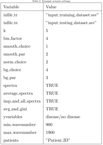
2.9.1. Example of operation

220

The following is an example of setting up and running the program in an R

environment. The user in this scenario wanted a binning of 4δ, S-G smoothing of order 2, vector normalisation and polynomial baseline correction of degree

3. They also wanted a wavenumber region of 900-1900 cm−1, and wished to

plot all available graphs. The descriptor being predicted was ”disease/no dis-225

ease”, which is a column with a 1 to denote a patient with the disease, and

2 for a patient without the disease. The desired split between training and

test sets was two thirds training - one third test. A script to do the splitting

is described in the Supporting Information. This script will by default split a

single CSV file into two files with training (input training dataset.ssv) and test-230

ing (input testing dataset.ssv) data respectively. The user intends to carry out

a 5-fold cross-validation of the training data. In this example scenario, there

are multiple spectra per patient, and the column denoting patient ID is called

”Patient ID”. The file user defined input.R would be set up according to Table

Table 2: Example scenario settings

Variable

Value

infile tr

”input training dataset.ssv”

infile te

”input testing dataset.ssv”

k

5

bin factor

4

smooth choice

1

smooth par

2

norm choice

2

bg choice

4

bg par

3

spectra

TRUE

average spectra

TRUE

imp and all spectra

TRUE

avg and gini

TRUE

yvariables

disease/no disease

min wavenumber

900

max wavenumber

1900

patients

”Patient ID”

and graphs would then be output as files into the current working directory. See

the flowchart for a list of the output files.

2.10. Example Data

240

As an example of the operation of the program, four datasets have been

analysed to find the best preprocessing parameters. These are all open-source

datasets available via the internet. The datasets were all FTIR spectra of food

items[34, 35, 36, 37]. The FTIR methods used included attenuated total

reflec-tion (ATR) and diffuse reflectance infrared Fourier transform (DRIFT). 245

2.10.1. Fruit Puree Example Dataset

The original fruit puree study[34] involved a PLS regression to predict

adul-teration of strawberry purees with various adulterants of other fruits or sugars.

The overall binary classes of the study were strawberry and non-strawberry,

with the adulterated samples being in the non-strawberry category. The study 250

used a training, tuning and test set for the regression. The classification was

then carried out by plotting the output of the PLS model, and cut-offs set by

95% confidence intervals. Using this methodology, overall results (mean of

sen-sitivity and specificity) were 96.5%, 93.5% and 94.3% for the training, tuning

and test sets respectively. There were 983 spectra in total, of which 351 were 255

pure strawberry.

2.10.2. Meats Example Dataset

The meat authenticity study[35] used ATR FTIR spectra of three different

types of meat. Chicken, pork and turkey samples were minced and the

spec-tra directly taken by placing the mince on an ATR crystal. There were two 260

spectra each of 20 samples, giving a total of 120 spectra. The classes were split

equally, giving 40 per meat type. The study used PLS regression to attempt to

detect varying levels of contamination of each meat into others. For example,

a regression was carried out to detect levels of turkey mixed with chicken. The

standard deviation of prediction errors (actual vs predicted composition) in that 265

2.10.3. Olive Oil Example Dataset

The olive oils study[36] combined multivariate analysis with ATR-FTIR, to

attempt to distinguish olive oils from different countries. The analysis methods

used were LDA based upon the scores from PLS, and a GA to determine variate 270

selection followed by LDA on the subset. The method of statistical analysis

and result collection was via a leave-one-out cross validation. The PLS-LDA

achieved a 96% success rate, and the GA-LDA achieved a 100% cross-validation

success rate.

The dataset itself consisted of 120 spectra, with 2 spectra per sample. Of 275

the samples, there were 10 from Greece, 17 from Italy, 8 from Portugal and 25

from Spain. The region of the IR spectrum used was 799-1897cm−1.

2.10.4. Coffee Example Dataset

The coffee study[37] focussed on the discrimination of two common types of

instant freeze-dried coffee,Arabica and Robusta. The original article explores 280

whether these types of coffee can be authenticated alone; and quantified in

mix-tures of the two. The spectra were collected via DRIFTS and ATR techniques.

LDA, PCA and regression were then employed as the data analysis methods.

LDA of the PCA scores yielded 100% accuracy of classification between the two

species. This classification was run with a roughly 4:1 training:test set split. 285

For the regression of differing proportions of each species, an R2 value of 0.99

and standard error of 1.2% were reported using internal cross-validation.

The available dataset (raw data) consisted of 56 samples (29 Arabica, 27

Robusta), collected in the 800-1900cm−1 _{region, using the DRIFTS technique.}

The data had a nominal resolution of around 3.85cm−1. 290

3. Results and Discussion

Grid searches were carried out to find best combinations of preprocessing.

The fitness evaluation function was the prediction accuracy statistic for the

search, every permutation of methods/parameters was tested on 96 randomly 295

selected training and test set splits. This was done to ensure a fair and accurate

portrayal of the abilities of the program. Results are given for best combinations

of preprocessing found for the data described above. In each subsection, tables

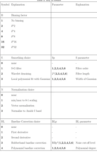
of the top 12 combinations are shown. A key to the table headings is given

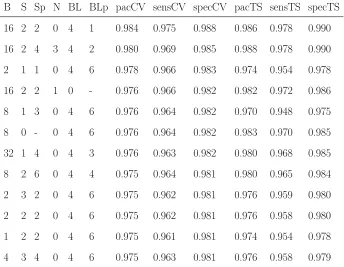
Table 3: Key to results

Symbol Explanation Parameter Explanation

B Binning factor

1 No binning

2 δ*2

4 δ*4

8 δ*8

16 δ*16

32 δ*32

S Smoothing choice Sp S parameter

0 none -

-1 S-G filter 1,2,3,4,5,6 Filter order

2 Wavelet denoising 2*(2,3,4,5,6) Filter length

3 Local polynomial fit with Gaussian 1,2,3,4,5,6 Width of Gaussian

N Normalisation choice

0 none

1 min/max to 0-1 scaling

2 Vector normalisation

3 Normalise to Amide I band

BL Baseline Correction choice BLp BL parameter

0 none -

-1 First derivative -

-2 Second derivative -

-3 Rubberband baseline correction RBp*(1,2,3,4,5,6) Noise cut-off level

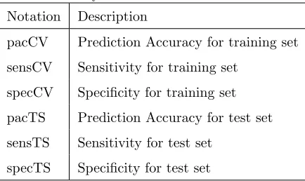
Table 4: Key to notation for statistical metrics

Notation Description

pacCV Prediction Accuracy for training set

sensCV Sensitivity for training set

specCV Specificity for training set

pacTS Prediction Accuracy for test set

sensTS Sensitivity for test set

specTS Specificity for test set

The statistical metrics used were sensitivity (true positive rate), specificity

(true negative rate) and prediction accuracy. The first two of these metrics are

widely used and have been defined elsewhere.[7]. Prediction accuracy, which is

defined in Equation 15, was used as the fitness function to identify the optimal

combinations of preprocessing routines. 305

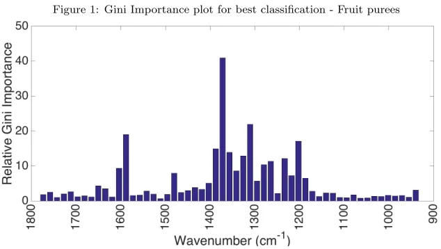
3.1. Fruit Example Dataset

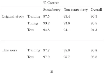
Table 5 shows the results for the binary classification of strawberry vs

non-strawberry purees. The results are on a par with the original study[34]. The

procedure in the original article is quite different from the procedure used to

generate our results. In this work, we used a direct classification with output 310

of important features. The original methodology was to use a PLS regression

both to find optimum number of PLS scores and to do a classification. Since

PRFFECT can directly produce a classification and report the best features, a

standard classification methodology was used by us. The original study used

three data partitions: training, tuning and test sets. As these were a third of 315

the data each, and RF training parameters are set to default values, we used two

thirds as a training set, and one third as a test set. A tuning set was not required

because RF is insensitive to small changes in its adjustable parameters and is

not prone to over-fitting.[7, 10, 38, 29] Default RF parameters were used for all

classifications reported in this article (500 trees per Random Forest, √ndesc.

320

more than 5 samples). Presented in Table 6 below is a direct comparison of our

best results from the top row of Table 5, and those of the original study.

The best combinations of preprocessing for this dataset always included a

binning factor of 4 or 8. When a factor of 8 was found to be preferable, it was 325

always followed with smoothing type 1 (S-G filter) with a smoothing parameter

of 5 (filter order). Smoothing types 1 and 3, S-G filter and local polynomial

Gaussian fit respectively, were the only two types to appear in the top dozen

results. The dataset shows an insensitivity to normalisation type, with all four

options appearing among the best classifiers. When it came to baseline correc-330

tion, every time the best choice was first derivative.

Overall, the results are very consistent across the measured metrics and CV

and test sets. The lowest statistic for both sets was specificity (equivalent to

”Non-strawberry” column in Table 6 below). However, our results were still

slightly in excess of the original study. Figure 1 shows the most important 335

Table 5: Results for fruit dataset

B S Sp N BL BLp pacCV sensCV specCV pacTS sensTS specTS

4

1 2

2

1

-

0.970

0.977

0.958

0.971

0.979

0.957

4

3 5

3

1

-

0.970

0.974

0.962

0.970

0.974

0.964

4

1 3

3

1

-

0.970

0.972

0.964

0.970

0.975

0.962

4

1 1

3

1

-

0.969

0.973

0.963

0.971

0.976

0.964

4

1 4

2

1

-

0.969

0.978

0.954

0.971

0.981

0.955

8

1 5

2

1

-

0.969

0.975

0.959

0.973

0.980

0.961

4

3 6

3

1

-

0.969

0.973

0.962

0.972

0.976

0.964

4

3 4

3

1

-

0.969

0.973

0.962

0.971

0.976

0.963

8

1 5

1

1

-

0.969

0.976

0.958

0.971

0.979

0.959

4

1 2

0

1

-

0.969

0.975

0.959

0.970

0.978

0.955

4

3 6

0

1

-

0.969

0.976

0.957

0.970

0.978

0.957

4

3 5

0

1

-

0.969

0.975

0.957

0.971

0.979

0.956

Table 6: Comparison of original results to this work, % correct classifications

% Correct

Strawberry Non-strawberry Overall

Original study Training 97.5

95.4

96.5

Tuning

93.2

93.8

93.5

Test

94.8

94.1

94.3

This work

Training 97.7

95.8

96.8

Figure 1: Gini Importance plot for best classification - Fruit purees

3.2. Meats Example Dataset

Since this dataset included 3 classes, metering the best possible preprocessing

was more cumbersome than with a binary classification. This is because there

are three separate sets of statistics which make up one result. Here, we have 340

simply averaged the results across all 3 meat types to find the best combinations.

A full database of all results obtained in this work can be found in the supporting

information. All found best combinations shown in Table 7 gave very strong

classification results. These are of course average results across pork, turkey

and chicken meats. As might be expected, pork was the easier meat to identify, 345

with many perfect results. The two bird meats were more difficult to separate

from one another, but overall the classifications performed very well.

The best combinations for this particular 3-way classification are very

in-teresting, especially the insensitivity to binning factor. All explored binning

factors are present in the top 12 results. The best combinations also appear 350

to be insensitive to smoothing choice and smoothing parameters. Again, all

possible smoothing types are present in the top 12. As for normalisations, 0

(no normalisation) was the preferred option. For baseline correction, option 4

(polynomial baseline correction) was seen in all but one of the top dozen. The

parameter space, with 6 appearing the most often.

Of all the results displayed in Table 7, specificity is the highest overall. This

could be due to the ease of which pork is separated from the two bird meats.

The slightly lower sensitivity values (although still very high) are probably due

to the difficulty of separating the turkey from the chicken meat. This gave a 360

very good test for the robustness of the random forest algorithm as a whole, in

that one class stood very far out from the others.

The main focus of the original paper[35] was to perform a regression of

varying compositions of meat mixtures. The spectra of the mixtures were not 365

available at the time of writing. Therefore, we have focussed on the classification

of different meats from the dataset. It is shown in the original article that PCA

was carried out on the whole meat data, and the loadings examined. The

loadings described show the strongest features in the 1550-1650 cm−1 _protein

region. There was also a smaller feature at 1740 cm−1 (lipid region). Figure 370

2 shows that this assessment fits well with what was found in this study. Of

course, it ought to be borne in mind that our best preprocessing combination

had a heavy binning factor of 16. Therefore, exact matches to wavenumber

Table 7: Results for meat dataset - average across 3 meat types

B

S Sp N BL BLp pacCV sensCV specCV pacTS sensTS specTS

16 2 2

0

4

1

0.984

0.975

0.988

0.986

0.978

0.990

16 2 4

3

4

2

0.980

0.969

0.985

0.988

0.978

0.990

2

1 1

0

4

6

0.978

0.966

0.983

0.974

0.954

0.978

16 2 2

1

0

-

0.976

0.966

0.982

0.982

0.972

0.986

8

1 3

0

4

6

0.976

0.964

0.982

0.970

0.948

0.975

8

0 -

0

4

6

0.976

0.964

0.982

0.983

0.970

0.985

32 1 4

0

4

3

0.976

0.963

0.982

0.980

0.968

0.985

8

2 6

0

4

4

0.975

0.964

0.981

0.980

0.965

0.984

2

3 2

0

4

6

0.975

0.962

0.981

0.976

0.959

0.980

2

2 2

0

4

6

0.975

0.962

0.981

0.976

0.958

0.980

1

2 2

0

4

6

0.975

0.961

0.981

0.974

0.954

0.978

4

3 4

0

4

6

0.975

0.963

0.981

0.976

0.958

0.979

Figure 2: Gini Importance plot for best classification - Meats

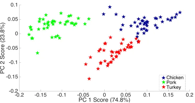
Figure 3 shows a PCA plot of the meat dataset, after being pre-processed 375

Figure 3: PCA plot for best preprocessing - Meats

plot present in the original study. Since the separation is better, it can be

concluded that the pre-processed data offers an improved classification.

3.3. Olive Oil Example Dataset

Similar to the meat example dataset, the olive oils dataset was a multi-380

class classification. In total there were four classes which represented country of

origin. Therefore Table 8 represents results averaged across these four classes.

A full database of results can again be found in the supporting information.

The results shown are for a 66:33 training:test split, as it is common to all

example datasets studied. The results were good overall, with specificity being 385

the strongest statistic. This may be expected since there were four classes

involved in the classification. Again, CV and TS results were very close.

Binning factors of 4 and 8 were preferred. The dataset appeared to be

rela-tively insensitive to smoothing choice and smoothing parameters. Normalisation

choice was similar, with normalisation to Amide I (option 3) being the only one 390

not appearing. It was clear however that baseline choice 1 (first derivative) was

strongly preferred.

Since the original study[36] employed a Leave-Two-Out Cross Validation

(LTOCV), we have repeated the classification with that methodology, using

A LTOCV was employed because there were two spectra per sample. While the

original study reported 100% correct classifications, our method misclassified

a total of 7 spectra from the 120 in the dataset. Three Spanish samples were

misclassified as Italian, two Spanish samples were misclassified as Portuguese

and two Portuguese samples misclassified as Italian. This meant a 94.2% correct 400

classification rate for our methodology. Although this is lower than the original

study, it is on a par with the overall results shown in Table 8.

Figure 4 shows the most important wavenumber descriptors for the four-way

classification. Some similarities can be seen between the histogram of the genetic

algorithm in the original paper (Figure 5a) and the Gini plot in our Figure 4. 405

It may be expected that these plots would show similar features, although they

were arrived at in very different ways.

Table 8: Results for olive oil dataset - average across 4 oil origins

B S Sp N BL BLp pacCV sensCV specCV pacTS sensTS specTS

8

0 -

1

1

-

0.964

0.928

0.975

0.965

0.927

0.975

4

3 6

2

1

-

0.963

0.929

0.974

0.963

0.927

0.973

4

3 6

1

1

-

0.963

0.929

0.974

0.958

0.923

0.970

4

1 2

2

1

-

0.962

0.927

0.974

0.963

0.934

0.973

4

3 5

2

1

-

0.962

0.924

0.973

0.963

0.931

0.974

4

3 4

2

1

-

0.961

0.923

0.972

0.965

0.937

0.975

8

0 -

2

1

-

0.961

0.916

0.973

0.969

0.940

0.978

4

1 6

0

1

-

0.960

0.924

0.972

0.966

0.939

0.976

4

1 3

0

2

-

0.960

0.927

0.972

0.964

0.930

0.974

4

3 4

1

1

-

0.960

0.922

0.972

0.961

0.927

0.972

4

1 4

1

1

-

0.960

0.921

0.972

0.971

0.947

0.979

Figure 4: Gini Importance plot for best classification - Olive Oils

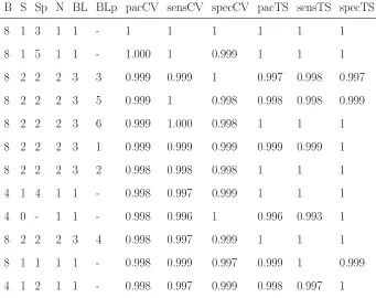
3.4. Coffee Example Dataset

Table 9 shows the classification results for the coffee dataset. This shows

clearly that the program performs just as well as the original study, even with 410

(effectively) a much smaller training set. Another interesting comparison to

make would be the areas of spectral distinction between the two species, as

identified in this work, and that of the original authors. This was originally

identified by examining PCA loadings. The Gini importance metric built into

our program should also show similar regions. The original study[37] found 415

areas of interest in the following regions: A large peak at around 1760 cm−1,

several loadings in the 1550-1750 cm−1 region, and several smaller features in

the 1150-1300 cm−1region. Figure 5 shows the Gini plot for the best

combina-tion of preprocessing parameters. As can be seen, the largest peak in the Gini

is in the same area as the original study’s PCA loadings. The other features 420

described by Briandet et. al. also match up rather well. Our best classification

happened to have a binning factor of 8 applied to the spectra. Therefore it

should be borne in mind that such heavily binned spectra by definition have

fewer datapoints overall.

It can be seen from Table 9 that the classification ofArabica vs Robusta was 425

near-perfect classifications. The reason there are small decreases in some statistics is

because these results were generated from averages of 96 separate training/test

set selections to ensure an un-biased test of the program. Binning factors of 8

and 4 were favourable. This translates to roughly a 30.8 cm−1_{and 15.4 cm}−1

ef-430

fective resolution respectively. The most favourable smoothing type was wavelet,

with a filter length of 4 (actual filter length is found by 2*Sp, as shown in

Ta-ble 3.) The best normalisation procedures were found to be min/max scaling

and vector normalisation. Interestingly, whenever min/max scaling was used,

the best baseline correction was always first derivative. Conversely, whenever 435

vector normalisation was used, the best baseline correction was the rubberband

technique. The rubberband technique appeared to be insensitive to the baseline

parameter, BLp (noise cut off level) for this dataset.

Overall, the program performed as well as the original study and showed 440

Table 9: Classification Results forArabica vsRobusta

B S Sp N BL BLp pacCV sensCV specCV pacTS sensTS specTS

8

1 3

1

1

-

1

1

1

1

1

1

8

1 5

1

1

-

1.000

1

0.999

1

1

1

8

2 2

2

3

3

0.999

0.999

1

0.997

0.998

0.997

8

2 2

2

3

5

0.999

1

0.998

0.998

0.998

0.999

8

2 2

2

3

6

0.999

1.000

0.998

1

1

1

8

2 2

2

3

1

0.999

0.999

0.999

0.999

0.999

1

8

2 2

2

3

2

0.998

0.998

0.998

1

1

1

4

1 4

1

1

-

0.998

0.997

0.999

1

1

1

4

0 -

1

1

-

0.998

0.996

1

0.996

0.993

1

8

2 2

2

3

4

0.998

0.997

0.999

1

1

1

8

1 1

1

1

-

0.998

0.999

0.997

0.999

1

0.999

4

1 2

1

1

-

0.998

0.997

0.999

0.998

0.997

1

Table 10: Results for coffee dataset - Comparison of methodologies

Source Correct Classifications

Original LDA classifier 100%

Figure 5: Gini Importance plot for best classification

4. Conclusions

Using PRFFECT, we were generally able to match or exceed the results

from the example studies. It was also a more streamlined process, and

pro-vided more information in some cases via the Gini Importance metric. It was 445

also possible to generate classification statistics automatically via the

built-in algorithms. PRFFECT shows great potential as a tool for spectroscopists

who wish to carry out classifications and explore various types of

preprocess-ing. Our group has already used it with success for diagnosing brain cancer

from serum FTIR samples.[7] It is particularly attractive since it is an all-in-one 450

package, no external preprocessing or statistical analysis of results is required.

Although PRFFECT dramatically simplifies the development of spectral

clas-sification models, it is not intended to be operated completely blindly. The

user must still make their own decisions about the reliability of the input data,

including whether the classes assigned to each sample are sufficiently well de-455

fined. Using the process-only version, it is possible to produce a dataset which

has been subject to several complex preprocessing procedures in one step. We

envision PRFFECT as being a popular and useful tool for spectroscopists of all

5. Independent testing

460

The software was independently tested by Dr John Mitchell of the

Depart-ment of Chemistry at the University of St. Andrews in the UK. At the time of

testing, the list of software dependencies in the manual was incomplete, but this

problem has now been fixed, as noted below. His comments in full:

“Thank you for giving me the opportunity to use your PRFFECT code. 465

I think it’s going to be a very useful resource for researchers looking to get

extra value from spectroscopic data at the interface between spectroscopy and

machine learning. I was aware of it from a poster at the ScotChem meeting in

Glasgow.

Having looked at the code, the manual is extensive and very helpful. I was 470

able to run the example datasets provided and they worked as expected. We

initially encountered some issues identifying which packages were to be

pre-installed. Thanks to your group for providing a definitive list of the R packages

required. I’m glad to see that the manual has been updated accordingly. I think

the current version of the manual is excellent and provides a clear and thorough 475

guide to the usage and capabilities of your excellent software.

I can confirm that the software runs as expected and that I expect it to

prove a valuable resource for the scientific research community.”

Acknowledgements

We thank Holly Butler and Robby Fritzsch for useful discussions. DSP and 480

BRS are grateful for use of the EPSRC funded ARCHIE- WeSt High

Perfor-mance Computer (http://www.archie-west.ac.uk, EPSRC Grant No. EP/K000586/1).

MJB and DSP would like to thank Scottish Enterprise for funding. MJB is

grateful for funding from EPSRC, Dstl, Rosemere Cancer Foundation, Brain

References

[1] D. I. Ellis, D. Broadhurst, D. B. Kell, J. J. Rowland, R. Goodacre, Rapid

and quantitative detection of the microbial spoilage of meat by fourier

transform infrared spectroscopy and machine learning, Appl. Environ.

Mi-crobiol. 68 (6) (2002) 2822–2828. 490

[2] M. G. Madden, A. G. Ryder, Machine learning methods for quantitative

analysis of raman spectroscopy data, in: OPTO Ireland, International

So-ciety for Optics and Photonics, 2003, pp. 1130–1139.

[3] F. Chauchard, R. Cogdill, S. Roussel, J. Roger, V. Bellon-Maurel,

Applica-tion of ls-svm to non-linear phenomena in nir spectroscopy: development of 495

a robust and portable sensor for acidity prediction in grapes, Chemometr.

Intell. Lab 71 (2) (2004) 141–150.

[4] J. R. Hands, G. Clemens, R. Stables, K. Ashton, A. Brodbelt, C. Davis,

T. P. Dawson, M. D. Jenkinson, R. W. Lea, C. Walker, et al., Brain

tu-mour differentiation: rapid stratified serum diagnostics via attenuated to-500

tal reflection fourier-transform infrared spectroscopy, J. Neurooncol 127 (3)

(2016) 463–472.

[5] C. L. Pickering, J. R. Hands, L. M. Fullwood, J. A. Smith, M. J. Baker,

Rapid discrimination of maggots utilising atr-ftir spectroscopy, Forensic

Sci. Int. 249 (2015) 189–196. 505

[6] T. Mudariki, R. Lea, G. Clemens, M. Baker, P59diagnostic application

of vibrational spectroscopy for the segregation of brain tumour cell lines

coupled with multivariate statistics, Neuro-oncology 16 (suppl 6) (2014)

vi10.

[7] B. R. Smith, K. M. Ashton, A. Brodbelt, T. Dawson, M. D. Jenkinson, 510

N. T. Hunt, D. S. Palmer, M. J. Baker, Combining random forest and

2d correlation analysis to identify serum spectral signatures for

[8] J. R. Hands, K. M. Dorling, P. Abel, K. M. Ashton, A. Brodbelt, C. Davis,

T. Dawson, M. D. Jenkinson, R. W. Lea, C. Walker, et al., Attenuated 515

total reflection fourier transform infrared (atr-ftir) spectral discrimination

of brain tumour severity from serum samples, J. Biophotonics 7 (3-4) (2014)

189–199.

[9] S. J. Barrington, H. Bird, D. Hurst, A. J. McIntosh, P. Spencer, S. H.

Pelfrey, M. J. Baker, Spectroscopic investigations of surface deposited bi-520

ological warfare simulants, in: SPIE Defense, Security, and Sensing,

Inter-national Society for Optics and Photonics, 2012, pp. 83580E–83580E.

[10] D. S. Palmer, N. M. O’Boyle, R. C. Glen, J. B. Mitchell, Random forest

models to predict aqueous solubility, J. Chem. Inf. Model 47 (1) (2007)

150–158. 525

[11] J. L. McDonagh, D. S. Palmer, T. v. Mourik, J. B. Mitchell, Are the

sublimation thermodynamics of organic molecules predictable?, J. Chem.

Inf. Model. 56 (11) (2016) 2162–2179.

[12] R. Diaz-Uriarte, S. de Andres, Gene selection and classification of

microar-ray data using random forest, BMC Bioinformatics 7. doi:{10.1186/

530

1471-2105-7-3}.

[13] D. R. Cutler, T. C. Edwards, Jr., K. H. Beard, A. Cutler, K. T. Hess,

Random forests for classification in ecology, Ecology 88 (2007) 2783–2792.

doi:{10.1890/07-0539.1}.

[14] F. Grosserueschkamp, A. Kallenbach-Thieltges, T. Behrens, T. Bruening, 535

M. Altmayer, G. Stamatis, D. Theegarten, K. Gerwert, Marker-free

au-tomated histopathological annotation of lung tumour subtypes by FTIR

imaging, Analyst 140 (7) (2015) 2114–2120. doi:10.1039/c4an01978d.

[15] J. Ollesch, D. Theegarten, M. Altmayer, K. Darwiche, T. Hager, G.

Stama-tis, K. Gerwert, An infrared spectroscopic blood test for non-small cell 540

adenocarcinoma, Biomedical Spectroscopy and Imaging 5 (2016) 129–144.

doi:10.3233/BSI-160144.

[16] J. Ollesch, M. Heinze, H. M. Heise, T. Behrens, T. Br¨uning, K. Gerwert,

It’s in your blood: spectral biomarker candidates for urinary bladder cancer 545

from automated FTIR spectroscopy, Journal of Biophotonics 7 (2014) 210–

221.

[17] H.-Z. Chen, G.-Q. Tang, W. Ai, L.-L. Xu, K. Cai, Use of Random Forest in

FTIR Analysis of LDL Cholesterol and Tri-Glycerides for Hyperlipidemia,

Biotechnology Progress 31 (6) (2015) 1693–1702. 550

[18] R Development Core Team, R: A Language and Environment for

Statisti-cal Computing, R Foundation for StatistiStatisti-cal Computing, Vienna, Austria,

ISBN 3-900051-07-0 (2008).

URLhttp://www.R-project.org

[19] A. Kohler, J. Sul´e-Suso, G. D. Sockalingum, M. Tobin, F. Bahrami, 555

Y. Yang, J. Pijanka, P. Dumas, M. Cotte, D. G. van Pittius, G. Parkes,

H. Martens, Estimating and Correcting Mie Scattering in

Synchrotron-Based Microscopic Fourier Transform Infrared Spectra by Extended

Mul-tiplicative Signal Correction, Appl. Spectrosc. 62 (3) (2008) 259–266.

[20] L. Kerr, B. Hennelly, A multivariate statistical investigation of background 560

subtraction algorithms for raman spectra of cytology samples recorded on

glass slides, Chemometr. Intell. Lab. Syst. 158 (Supplement C) (2016) 61

– 68.

[21] C. Beleites, V. Sergo, hyperspec: a package to handle hyperspectral data

sets in r, R package v. 0.98-20120725. 565

[22] B. K. Alsberg, A. M. Woodward, M. K. Winson, J. Rowland, D. B. Kell,

[23] D. Zhan, S. Sun, Q. Zhou, Z. Qin, Wavelet denoising and optimization of

two-dimensional correlation ir spectroscopy, Spectrosc. Spect. Anal. 24 (12)

(2004) 1549–1552. 570

[24] I. Daubechies, Orthonormal bases of compactly supported wavelets, Comm.

Pure Appl. Math 41 (7) (1988) 909–996.

[25] A. Savitzky, M. J. Golay, Smoothing and differentiation of data by

simpli-fied least squares procedures., Anal. Chem. 36 (8) (1964) 1627–1639.

[26] M. J. Baker, J. Trevisan, P. Bassan, R. Bhargava, H. J. Butler, K. M. 575

Dorling, P. R. Fielden, S. W. Fogarty, N. J. Fullwood, K. A. Heys, et al.,

Using fourier transform ir spectroscopy to analyze biological materials, Nat.

Protoc. 9 (8) (2014) 1771–1791.

[27] C. A. Lieber, A. Mahadevan-Jansen, Automated method for subtraction of

fluorescence from biological raman spectra, Appl. Spectrosc. 57 (11) (2003) 580

1363–1367.

[28] L. Breiman, Random forests, Mach. Learn. 45 (1) (2001) 5–32.

[29] L. D. Hughes, D. S. Palmer, F. Nigsch, J. B. O. Mitchell, Why are some

properties more difficult to predict than others? A study of QSPR models

of solubility, melting point, and log P, J. Chem. Inf. Model. 48 (2008) 585

220–232.

[30] D. S. Palmer, M. Miˇsin, M. V. Fedorov, A. Llinas, Fast and general method

to predict the physicochemical properties of druglike molecules using the

integral equation theory of molecular liquids, Mol. Pharm. 12 (9) (2015)

3420–3432. 590

[31] E. O. Cannon, A. Bender, D. S. Palmer, J. B. O. Mitchell,

Chemoinformatics-based classification of prohibited substances employed

[32] A. Liaw, M. Wiener, Classification and regression by randomforest, R news

2 (3) (2002) 18–22. 595

[33] B. R. Smith, M. J. Baker, D. S. Palmer, PRFFECT User Manual,

Univer-sity of Strathclyde, Glasgow, UK (2017).

URLhttps://github.com/Palmer-Lab/PRFFECT

[34] J. Holland, E. Kemsley, R. Wilson, Use of fourier transform infrared

spec-troscopy and partial least squares regression for the detection of adulter-600

ation of strawberry purees, J. Sci. Food Agr. 76 (2) (1998) 263–269.

[35] O. Al-Jowder, E. Kemsley, R. Wilson, Mid-infrared spectroscopy and

au-thenticity problems in selected meats: a feasibility study, Food Chem.

59 (2) (1997) 195–201.

[36] H. S. Tapp, M. Defernez, E. K. Kemsley, Ftir spectroscopy and multivariate 605

analysis can distinguish the geographic origin of extra virgin olive oils, J.

Agr. Food Chem. 51 (21) (2003) 6110–6115.

[37] R. Briandet, E. K. Kemsley, R. H. Wilson, Discrimination of arabica and

robusta in instant coffee by fourier transform infrared spectroscopy and

chemometrics, J. Agr. Food Chem. 44 (1) (1996) 170–174. 610

[38] D. S. Palmer, J. B. O. Mitchell, Is experimental data quality the

limit-ing factor in predictlimit-ing the aqueous solubility of druglike molecules?, Mol.