Leveraging big data for fuel oil consumption modelling

Leveraging Big Data for Fuel Oil Consumption Modelling

Christos Gkerekos, University of Strathclyde, Glasgow/UK, christos.gkerekos@strath.ac.uk

Iraklis Lazakis, University of Strathclyde, Glasgow/UK, iraklis.lazakis@strath.ac.uk

Stylianos Papageorgiou, Lomar Shipping, London/UK, stylianos.papageorgiou@lomarshipping.com

Abstract

Fuel oil consumption constitutes over 25% of a vessel’s overall running costs. Therefore, accurately forecasting, and optimising fuel costs majorly impacts a vessel’s operation sustainability and profitability. This paper presents data-driven, multivariate main engine fuel consumption models leveraging the vast amount of data currently being recorded onboard vessels. Different data-driven modelling methodologies, such as shallow neural networks, deep neural networks, support vector machines, and random forest regressors are presented and implemented, comparing results. The suggested multivariate modelling allows the uncovering of latent interconnections that increase the robustness of the model in varied operating conditions.

1. Introduction

Efficient operations of vessels are desired from various maritime industry stakeholders such as ship operators, Classification Societies, consultancy companies, maritime regulators, and policy makers. Efficient operations lead to both decrease of Green House Gases (GHGs) and operating cost reduction. Τhis desire can be justified by financial reasons, such as reduced fuel consumption and decreased maintenance costs. Ronen (2011) notes that when bunker fuel price is at around 500 USD per ton, fuel costs correspond to approximately 75% of the total operating cost of a large containership. Accordingly, Stopford (2009) notes that fuel oil consumption constitutes approximately two-thirds of a vessel’s voyage costs and over one-quarter of a vessel’s overall running costs. For this reason, shipping companies are lately focusing on implementing fuel efficiency measures. In order to monitor fuel efficiency and eventually offer a formalized optimization approach to fuel consumption, a suitable modelling framework that can take into account relevant variables (measurements) and their correlation is required.

The purpose of this study is to develop a fuel consumption model that utilizes data obtained from the noon-reports that are transmitted daily back to shore. Compared to other approaches where modelling is performed using the data acquired through specialized sensors, implementation of this approach has an infinitesimal cost as no additional hardware is required. Through that, scaling this methodology from vessel- to fleet-level becomes a triviality. Additionally, unlike methods that utilize data from sea- and shop-trials for modelling, this method provides the flexibility of permitting only the utilization of data corresponding to a specific period and/or vessel’s operational profile for modelling.

2. Background

This section provides an overview of scientific literature, pertinent to this paper. First, methodologies relevant to fuel efficiency and fuel consumption modelling are included. Besides, a synopsis of data-driven techniques pertinent to the modelling requirements of this paper are presented.

Beşikçi et at (2016) suggested the use of Artificial Neural Networks (ANNs) for the prediction of ship fuel consumption at various operational conditions. Additionally, a Decision Support System (DSS) is elaborated for real-time, energy efficient operations. The suggested methodology is compared against Multiple Regression (MR) analysis, displaying superior results. Meng et al. (2016) suggest a data pre-processing methodology based on outlier-score-based data. Following that, two regression models are developed in order to link available data to fuel consumption. The first model connects the ship's fuel consumption with its speed and displacement. The second model builds on the first, utilising the information provided by the first while also including weather conditions. They validated the work performed utilising noon-report data from 13000-TEU containerships.

Cichowicz et al. (2015) provide a methodology for first-principles, time-domain modelling of main and auxiliary engines for assessment of life-cycle ship performance and energy efficiency. Speed and draught are taken into consideration, along with hull fouling and deterioration of engine performance. Sea state is included implicitly by considering an additional ME load. The methodology was demonstrated using data from 3700-TEU containership. Coraddu et al. (2017) performed a comparison of white, grey, and black box models for the estimation of fuel consumption, concluding that grey-box models can effectively forecast fuel consumption when only limited historical data are available.

Trodden et al. (2015) focuses on data pre-processing and suggests a methodology, ancillary to the ones elaborated above, for splitting available ship data into steady-state chunks that can then be used for fuel efficiency monitoring.

From the above, modelling of vessels’ fuel oil consumption is an active research field with multiple different approaches being realised concurrently. Up to now, modelling attempts seem to be focused either on the evaluation of noon-report data using first-principles modelling or a priori knowledge, or on a noon-report dataset or the use of high-frequency data along with a machine-learning approach. This paper aims to examine how noon-report data can be combined with different machine learning approaches and whether acceptable results can be achieved through that.

3. Methodology

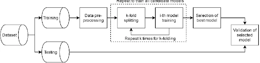
The methodology elaborated in this section concerns a) the description of a suitable pre-processing technique for the acquired dataset; b) the derivation of multiple models following different modelling methodologies; c) the optimisation of the hyperparameters of these models; and d) the comparison of those models so that modelling techniques that offer the best performance are identified. Fig.1 shows the suggested methodology with all suggested modules and their relevant interconnections.

Fig.1: Suggested methodology

3.1 Data pre-processing

accurately be used as predictors for the FO consumption of the vessel.

All numerical attributes in the dataset are standardized by removing the mean and scaling to unit variance. Therefore, for a numerical attribute 𝑥, a standardised attribute 𝑥′ is produced by

𝑥′ =𝑥 − 𝜇 𝜎

where 𝜇 is the mean value of all values belonging to that attribute and 𝜎 its standard deviation. All attributes are standardised so that all attributes can contribute equally to the objective function that is used for model training.

3.2 Modelling methodologies

All modelling methodologies presented below are methodologies relating to regression analysis. Regression analysis is a set of statistical processes that aims to derive a relationship between several dependent variables (predictors) and an independent (target) variable.

Regression models can be derived with a varying level of complexity and consequently accuracy of results. Therefore, possible methods span a wide range of options, from closed-form linear models to deep (i.e. multi-layered) neural networks.

Different modelling approaches can be split into parametric and non-parametric. Parametric models assume some finite set of parameters 𝜃. Given these parameters, any future prediction, 𝑥, are independent of the observed dataset 𝐷 so that:

𝑃(𝑥|𝜃, 𝐷) = 𝑃(𝑥|𝜃)

In other words, 𝜃 is assumed to capture all variance contained in the dataset 𝐷.

Therefore, even if the complexity of a dataset is unbounded (potentially infinite), the complexity of the model is bounded. Linear models such as linear regression and Support Vector Regressors (SVRs) with a linear kernel are parametric models.

In contrast to that, non-parametric models assume that the dataset distribution cannot be defined using any finite number of parameters. Therefore, the amount of information that 𝜃 can capture grows with the number of training data points in dataset 𝐷. Decision tree regressors, random forest regressors and SVRs with a Radial Basis Function (RBF, a non-linear kernel used in support vector machines to allow the learning of non-linear mappings) kernel are considered non-parametric as the number of parameters grows with the size 𝐷.

Finding the optimal model-derivation methodology is non-trivial as this is affected, among others, by the quantity and quality of available data, and the nature (also complexity) of the problem at hand.

3.2.1 Decision tree regressors

Decision tree regressors are a non-parametric, supervised regression method. Decision tree regressor models learn simple decision rules inferred from the dataset features and predict the value of the target variable through those, Hastie et al. (2009).

3.2.2 Random forest regressors

Random forests are based on the bagging (bootstrap aggregating) meta-algorithm, a technique that aims to reduce the variance of an estimated prediction function, Hastie et al. (2009). In the case of random forest regressors, a number of de-correlated decision tree regressors are produced based on the available training set. Then, the output of the random forest regressor is calculated by averaging the results of individual decision trees.

3.2.3 Support vector machines

Support Vector Machines (SVMs) in their simplest form constitute a two-class classifier in cases where the two classes are linearly separable. SVMs work by deriving the optimal hyperplane, i.e. the hyperplane that offers the widest possible margin between instances of the two classes. (In geometry, a hyperplane is a subspace whose dimension is one less than that of its ambient space. For example, in the case of observations with two attributes (therefore positioned in a 2D space), their separating plane will be one-dimensional, i.e. a line.) Their functionality can be extended by the introduction of a non-linear kernel, allowing them to learn non-non-linear mappings, i.e., classify between non-non-linearly separable classes, Theodoridis (2008).

SVMs can also be built as regressors, Smola et al. (2004). Support Vector Regressors (SVRs) work in a similar way, this time trying to fit a hyperplane that accurately predicts the target values of training samples within a margin of tolerance 𝜀.

3.2.4 Shallow & deep neural networks

Artificial Neural Networks (ANNs) are computing systems, inspired by the way biological nervous systems work. Various ANN architectures exist, offering superior performance at many machine learning tasks, including classification and regression. ANNs are extremely versatile as they can accurately model complex non-linear behaviours.

ANNs are based on an interconnected group of connected units (neurons) where each connection between these units can transmit a signal from one to another. The receiving unit can process that signal and then pass it on to the next unit.

Two important parameters of ANNs are the number of hidden (between input and output) layers and the number of units per layer. Excluding the input and output layers that always exist, different architectures call for different number of hidden layers and units. Accordingly, different activation functions can be implemented, altering the complexity learnable by the model.

Consequently, depending on the number of layers implemented, ANNs can be classified as shallow and deep. While no formal rule exists to separate shallow and deep neural networks, Schmidhuber (2015), usually networks that have more than 1 hidden layer are considered deep. As the number of layers increases, the model can “learn” more non-linear behaviours. At the same time, training becomes more computationally expensive and the risk of overfitting the dataset also increases.

3.3 Model hyperparameter optimisation

evaluated (especially in the case of multiple tuneable hyperparameters per model). Another approach is to employ a random search implementation. There all hyperparameter ranges are randomly sampled, usually producing more accurate results given a predefined number of draws, Bergstra and Bengio (2012).

3.4 Selection of best model

In order to reasonably ensure that selected hyperparameter values are actually close to optimal and not merely overfitting the model, a 𝑘-fold technique is implemented. There, the training dataset is split into 𝑘 subsets and an iterative process runs 𝑘 times, using 𝑘 − 1 subsets for training and the remaining one for testing. Therefore, for each hyperparameter combination several results are obtained and averaged. Using the same technique for all models, allows us to identify the model that performs best while at the same time ensuring good generalisation capabilities.

4. Application description, results, and discussion

In this section, a case study utilising noon-report data from a reefer vessel is included. 834 data points were available, corresponding to approximately 2.5 years of noon-report data. An overview of the available attributes can be seen below in Table I.

Table I: Noon-report measurements used for model training

# Name Units # Name Units

1 Speed (noon) Knots 8 Sea state (1-12)

2 Engine speed RPM 9 Sea direction degrees, summed

in 12 bins 3 Sea current

(relative to vessel)

knots 10 Slip %

4 Wind force (1-12) 11 Draft fwd m

5 Wind direction degrees, summed in 12 bins

12 Draft aft m

6 Daily M/E FOC tn 13 Daily steam hours hr

7 Daily distance run nm

These data were pre-processed to keep only points where all required attributes were available and where the following conditions were met:

• Daily steam hours > 10 • Daily M/E FOC > 5 tn • Speed (noon) > 8 nm • Engine speed > 20 RPM

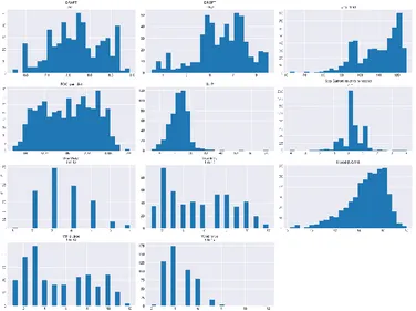
These values were selected to only take into account data points that correspond to relatively steady state conditions, without significant transient instances, e.g. manoeuvring. Following this pre-processing, 512 data points were kept. A histogram of the selected attributes is shown in Fig.2. Additionally, Daily M/E FOC and Daily distance run were combined into a single “FOC per distance run” attribute, in order to more accurately represent model target. Then, 20% of the data were kept aside for model validation, leaving the rest for model training. As a brief investigation of the available training dataset, a correlation matrix was obtained, focusing on how “FOC per distance run” correlates with other attributes, shown in Table II.

model produced at each fold. The Neural Network model utilizing default hyperparameters is not included as the relevant model failed to converge.

Fig.2: Histogram plots of attributes used for model input after pre-processing

Table II: Correlation of “FOC per distance run” to other attributes Attribute Correlation

Engine speed 0.777729 Sea State 0.491557 Slip 0.470700 Wind force 0.429272 Speed (noon) 0.398368 Draft aft 0.129491 Draft fwd -0.012756 Sea direction -0.053529 Wind direction -0.079869 Sea current -0.279159

An overview of obtained results is presented in the box plots of Fig.3 shown below. The value inside each box corresponds to the median (second quartile) score of this model in 𝑘-folding, the top and bottom of the box respectively correspond to the first and third quartiles. The whiskers represent the lowest point of data within 1.5 Interquartile Range (IQR) of the lowest quartile and the highest point of data within 1.5 IQR of the upper quartile. Accordingly, the mean of the dataset is noted by a triangle. Data points beyond the whisker range as shown individually as small circles. A logit y-axis is used to emphasize model performance in the range of 85-95%, i.e. the most interesting range as all candidate models are performing around that range.

Fig.3: Box plot of 𝑅2 _{score obtained from different models and hyperparameters in 𝑘-folding}

Moreover, neural networks performed rather poorly in this case study. As noted above, default hypermeters yielded a model that failed to converge. While models with hyperparameters obtained through random search fared better, results were still significantly worse off that those obtained through other modelling techniques. An additional key remark is how increasing the depth of the neural network did not provide better results and, in fact, delivered worse mean accuracy in all attempted cases.

The best accuracy was obtained by random forests and RBF-based SVMs, both after optimizing their hyperparameters. Comparing the two models, the SVM model yielded higher mean/median scores. However, it should be noted that the random forest model yielded a lower spread between different folds (i.e. less elongated box and whiskers).

Having selected the model that performed best in k-folding, the same parameters are now tested in the dataset held aside for validation. There, a score of 𝑅2=0.8230, corresponding to an accuracy of 82.3% was obtained, ensuring that the model developed generalizes well.

5. Conclusions

This paper presented a data-driven methodology of estimating main engine fuel oil consumption of sailing vessels through the use of noon-report data. An overview of the current state of research in this field was provided, followed by a compact description of the main idea behind multiple regression modelling approaches.

To conclude, future research includes examination of this problem in the existence of denser datasets and whether that alters the model ranking described above. Furthermore, additional modelling techniques can also be examined.

Acknowledgements

The work presented in this paper is partially funded by INCASS and ISEMMS projects. INCASS Project has received research funding from the European Union’s Seventh Framework Program under grant agreement no 605200. ISEMMS project has received research funding from Innovate UK under Project No. 102435. This publication reflects only the authors’ views and European Union/Innovate UK are not liable for any use that may be made of the information contained within.

References

BERGSTRA, J.; BENGIO, Y. (2012), Random search for hyper-parameter optimization, J. Machine Learning Research 13, pp.281-305

BEŞIKÇI, E.B.; ARSLAN, O.; TURAN, O.; ÖLÇER, A.I. (2016), An artificial neural network based decision support system for energy efficient ship operations, Computers & Operations Research 66, pp.393-401

BIALYSTOCKI, V.; KONOVESSIS, D. (2016), On the estimation of ship's fuel consumption and speed curve: A statistical approach, J. Ocean Engineering and Science 1/2, pp.157-166

CICHOWICZ, J.; THEOTOKATOS, G.; VASSALOS, D. (2015), Dynamic energy modelling for ship life-cycle performance assessment, Ocean Engineering 110/B, pp. 49-61

CORADDU, A.; ONETO, L.; BALDI, F.; ANGUITA, D. (2017), Vessels fuel consumption forecast and trim optimisation: a data analytics perspective, Ocean Engineering 130, pp. 351-370

GLANTZ, S.A.; SLINKER B.K. (1990), Primer of Applied Regression and Analysis of Variance, McGraw-Hill

HASTIE, T.; TIBSHIRANI, R.; FRIEDMAN, J. (2009), The Elements of Statistical Learning: Data Mining, Inference, and Prediction, Springer

LU, R.; TURAN, O.; BOULOUGOURIS, E.; BANKS, C.; INCECIK, A. (2015), A semi-empirical ship operational performance prediction model for voyage optimization towards energy efficient shipping, Ocean Engineering 110/B, pp.18-28

MENG, Q.; DU, Y.; WANG, Y. (2016), Shipping log data based container ship fuel efficiency modeling, Transportation Research Part B: Methodological 83, pp.207-229

PEDREGOSA, F.; VAROQUAUX, G.; GRAMFORT, A.; MICHEL, V.; THIRION, B.; GRISEL, O.; BLONDEL, M.; PRETTENHOFER, P.; WEISS, R.; DUBOURG, V.; VANDERPLAS, J.; PASSOS, A.; COURNAPEAU, D.; BRUCHER, M.; PERROT, M.; DUCHESNAY, E. (2011), Scikit-learn: Ma-chine Learning in Python, J. MaMa-chine Learning Research, 12, pp.2825-2830

RONEN, D. (2011), The effect of oil price on containership speed; fleet size, J. Operational Research Society 62/1, pp.211-216

SCHMIDHUBER, J. (2015), Deep Learning in Neural Networks: An Overview, Neural Networks 61, pp. 85-117

14/3, pp.199-222

STOPFORD, M. (2009), Maritime Economics, Routledge

THEODORIDIS, S. (2008), Pattern Recognition, Elsevier