City, University of London Institutional Repository
Citation
:
Zhu, R., Wang, Z., Sogi, N., Fukui, K. and Xue, J-H. (2019). A Novel Separating
Hyperplane Classification Framework to Unify Nearest-class-model Methods for
High-dimensional Data. IEEE Transactions on Neural Networks and Learning Systems,
This is the accepted version of the paper.
This version of the publication may differ from the final published
version.
Permanent repository link:
http://openaccess.city.ac.uk/id/eprint/23006/
Link to published version
:
Copyright and reuse:
City Research Online aims to make research
outputs of City, University of London available to a wider audience.
Copyright and Moral Rights remain with the author(s) and/or copyright
holders. URLs from City Research Online may be freely distributed and
linked to.
City Research Online:
http://openaccess.city.ac.uk/
[email protected]
A Novel Separating Hyperplane Classification
Framework to Unify Nearest-class-model Methods
for High-dimensional Data
Rui Zhu, Ziyu Wang, Naoya Sogi, Kazuhiro Fukui,
Member, IEEE,
and Jing-Hao Xue
Abstract—In this paper, we establish a novel separating hyper-plane classification (SHC) framework to unify three nearest-class-model methods for high-dimensional data: the nearest subspace method (NSM), the nearest convex hull method (NCHM) and the nearest convex cone method (NCCM). Nearest-class-model methods are an important paradigm for classification of high-dimensional data. We first introduce the three nearest-class-model methods and then conduct dual analysis for theoreti-cally investigating them, to understand deeply their underlying classification mechanisms. A new theorem for the dual analysis of NCCM is proposed in this paper, through discovering the relationship between a convex cone and its polar cone. We then establish the new SHC framework to unify the nearest-class-model methods based on the theoretical results. One important application of this new SHC framework is to help explain empirical classification results: why one class model has better performance than others on certain datasets. Finally, we propose a new nearest-class-model method, the soft NCCM, under the novel SHC framework to solve the overlapping class model problem. For illustrative purposes, we empirically demonstrate the significance of our SHC framework and the soft NCCM through two types of typical real-world high-dimensional data, the spectroscopic data and the face image data.
Index Terms—Classification, convex cone, convex hull, dual analysis, separating hyperplane, subspace.
I. INTRODUCTION
A
Category of popular generative classifiers to classifyhigh-dimensional data is the nearest-class-model meth-ods, also known as the class modelling methods in the chemo-metrics community or the subspace methods in the machine learning and pattern recognition communities. In the nearest-class-model methods, we construct a class model for each class from the training samples of that class, independently of other classes; a test sample is assigned to the class with the highest similarity between the sample and the class model.
Three class models have been studied in the literature, the principal component (PC) subspace, the convex hull model
R. Zhu is with the Faculty of Actuarial Science and Insurance, City, University of London, London EC1Y 8TZ, UK. E-mail: [email protected]
Z. Wang is with the Department of Security and Crime Science and the Department of Statistical Science, University College London, London WC1E 6BT, UK. E-mail: [email protected]
N. Sogi and K. Fukui are with the Department of Computer Science, University of Tsukuba, Tsukuba, Japan. Email: [email protected]; [email protected]
J.-H. Xue is with the Department of Statistical Science, University College London, London WC1E 6BT, UK. E-mail: [email protected]
This work was partially supported by University College London’s Security Science Doctoral Training Centre under Engineering and Physical Sciences Research Council (EPSRC) grant EP/G037264/1.
and the convex cone model. PC subspace is a widely-used class subspace. The PC subspace of a class is built through principal component analysis (PCA) of the training samples of that class, such that a class is represented by a low-dimensional linear subspace spanned by a small number of learning PCs which present the most variable information in the class. Hence the PC subspace has been widely used as a class representation for high-dimensional data. Soft independent
modelling of class analogy (SIMCA) [1]–[6] in chemometrics
and the mutual subspace method (MSM) [7]–[10] and the
nearest subspace classifier (NSC) [11]–[14] in pattern
recog-nition are famous examples of PC-subspace-based classifiers. In SIMCA and NSC, the dissimilarity measure is related to the Euclidean distance between a test sample and a PC subspace; in MSM, it is the canonical angle between them. It is, however, not necessary to use subspaces to represent classes. The geometric convex model representation is another popular class representation approach for classification tasks. The geometric convex model for a class is constructed by a linear combination of class samples, with certain constraints on the linear combination coefficients.
The convex hull model [15]–[19] is one geometric model
that attracts a lot of attention recently. Nalbantov et al. [15]
propose the nearest convex hull classification, which uses a convex hull model to represent a class and classifies a test sample to the class with the nearest convex hull. The convex hull model of a class is constructed by the convex combination, i.e. the linear combination with nonnegative and sum-to-one constraints on the coefficients, of the training samples of that class. The dissimilarity measure is the Euclidean distance from
a test sample to a convex hull [15].
The convex cone model has also been used as class
repre-sentation for face recognition [14], [20]. A convex cone model
is constructed by the conic combinations of the class samples, i.e. the linear combinations with nonnegative coefficients.
Kobayashi et al. [20] propose the cone-restricted subspace
method, using the angle between a test sample and a convex cone for classification.
The restricted area is bounded by the class samples that are used to construct the convex models. The convex hull model adopts the convex constraints on the linear combination coefficients. However, the convex constraint is often too tight in the sense that the classes often extend well beyond the
convex hulls [17]. Considering the tightness of a model, a
convex cone model lies in between a linear subspace model and a convex hull model. A convex cone is more restricted than a linear subspace because of the nonnegative constraints on the coefficients, while is looser than a convex hull because the conic combination constraint is looser than the convex combination constraint.
The geometric convex models have shown superior
classifi-cation performances to the PC subspace [15], [20]. However,
theoretically why and when this will happen is barely studied
in literature. Therefore, in this paper, we aim to theoretically
investigate and unify three nearest-class-model classification methods which respectively use the PC subspace, the convex hull and the convex cone. Under the unified framework, we are able to explain why for certain datasets one class model is superior to the others in terms of empirical classification per-formance. In addition, we aim to develop new nearest-class-model methods under this framework to better classify data with specific properties, e.g. with overlapping class models.
To make the theoretical investigation more straightforward, we use the distance as the dissimilarity measure. In this fashion, the PC subspace representation leads to a nearest subspace
method (NSM) [11]; the convex hull model leads to a nearest
convex hull method (NCHM) [15]; and the convex cone model
leads to a nearest convex cone method (NCCM), which is
similar to the method in [20].
We first establish the novel separating hyperplane classi-fication (SHC) framework to unify the nearest-class-model methods through the separating hyperplanes as a common platform. To achieve this, we shall investigate the correspond-ing hyperplane-based classifiers to NSM, NCHM and NCCM,
through thedual analysis of their minimum distance problems.
We first introduce the dual analysis for NSM and NCHM in literature and then show a new theoretical result of the dual analysis for NCCM through discovering the relationship between a convex cone and its polar cone. This relationship is analogous to that between a subspace and its orthogonal complement. We shall show that the minimum distance from a test sample to a class model is equivalent to the maxi-mum distance from that sample to a hyperplane. Thus for each class model, we can find one separating hyperplane that separates the test sample from the class models. The test sample is then classified to the class with its nearest hyperplane. Therefore different class models are unified by the separating hyperplanes which can be simply described by their normal vectors and biases. However, we note that formulating a nearest class problem using hyperplanes does
not bring advantages in computation [21].
Based on the SHC framework, we can then explain em-pirical classification results by investigating the discriminative abilities of the normal vectors associated with the separating hyperplanes. We shall show that the normal vectors of the sep-arating hyperplanes are of great importance to classification:
the more discriminative the normal vectors are, the better the classification.
It is worth noting that our SHC framework is different from the extensions of support vector machine (SVM) based on a pair of separating hyperplanes in one-sided or two-sided
best fitting hyperplane classifiers [22], generalised eigenvalue
proximal SVM [23] or twin SVM [24]. In [22]–[24], the pair of
separating hyperplanes are found for the pair of class models and fixed for all the test samples, making the classification boundary linear for linear kernels. In contrast, the pair of separating hyperplanes in our SHC framework vary with test samples, making the classification boundary nonlinear.
We then propose a new classifier, the soft NCCM, under the SHC framework by imposing proper constraints to solve the overlapping class model problem. In real applications, it is possible to have overlapping class models and the class mem-berships of the test samples locating in the overlapping area are ambiguous. The new soft NCCM utilises the discriminative between-class information when constructing the class cones and can eliminate the overlapping area between the cones. The test instances locating in the overlapping area can then be better classified unambiguously.
For illustrative purposes, we apply NSM, NCHM, NCCM and soft NCCM to two types of typical high-dimensional data, the spectroscopic data and the face image data. We shall show the effectiveness of the new SHC framework in explaining the empirical classification results on these real data. We shall also show the superior classification performance of the new soft NCCM classifier over other methods to classify these data.
The contributions of our work are threefold.
1) We develop new theoretical results of the dual analysis of NCCM, by discovering the relationship between a convex cone and its polar cone.
2) We establish a novel separating hyperplane classifica-tion (SHC) framework to unify and easily compare the nearest-class-model methods. Empirically, the new SHC framework can help explain why a class model is superior for certain datasets; and methodologically, it can help to design more sophisticated nearest-class-model methods with better classification performance. 3) We propose a new nearest-class-model method, the
soft NCCM, under the SHC framework to solve the overlapping class model problem.
II. NEAREST-CLASS-MODEL METHODS
In this section we introduce the three nearest-subspace-methods, NSM, NCHM and NCCM, with illustrative examples in a two-dimensional feature space.
A. PC subspace model: NSM
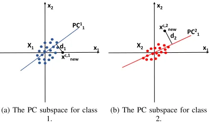
The nearest subspace method (NSM) models each class by a principal component (PC) subspace which can be obtained by applying the singular value decomposition on the centred training set of one class. A test instance is then classified to the nearest class by comparing its Euclidean distances to the
two class subspaces. Fig. 1 shows an illustrative example of
x1
x2
PC1 1
X1
xc,1 new
d1
(a) The PC subspace for class 1.
x1
x2
PC2 1
X2
xc,2 new
d2
[image:4.612.68.283.64.190.2](b) The PC subspace for class 2.
Fig. 1: An illustrative example of NSM in a 2D space.
straight lines are the PC class subspaces of the two classes, respectively, which are constructed by the first PCs. The
Euclidean distances fromxnewto the two class subspaces are
shown as d1 andd2, respectively. In this example, we assign
xnew to class 1 sinced1< d2. Note that we use two plots to
represent the PC subspaces of the two classes, respectively, in order to achieve better visualisation. The technical details of NSM are described as follows.
Definition II.1. Subspace.SupposeS ={xi}Ni=1 is a subset
of Rp. The setL(S) ={v: v =
N
P
i=1
αixi|xi∈S, αi∈R},
called the subspace generated by S, consists of all vectors in
Rp which are linear combinations of vectors in S. We also
say that the vectors in S span the subspaceL(S).
In the training phase, the nearest subspace method (NSM) builds class subspaces for the classes separately using PCA.
We denote Xk ∈ RNk×p as the training set of class k
(k= 1,2for two-class classification), whereNkis the number
of training samples and each row of Xk represents a p
-dimensional training sample. The PC subspace for the kth
class can be obtained from applying the reduced singular value
decomposition to the column-centred Xk:Xck =UkΛkVTk,
where the rows of Uk ∈ RNk×qk denote the normalised PC
scores; the columns ofVk ∈Rp×qkdenote the PCs; andΛ
kis
a diagonal matrix of singular values {λ1≥λ2≥. . .≥λqk}.
The rk-dimensional (rk ≤ qk) PC subspace L(Wk) is
spanned by the first rk PCsWk ∈Rp×rk.
In the test phase, a new sample xnew ∈R1×p is assigned
according to the distance from xc,knew to the class subspace
L(Wk), wherexc,knew is the centredxnew by the mean vector
ofXk. The distance is defined as the minimum distance from
xc,k
new to the vectors in L(Wk):
dLk = min
αL
k
||xc,knew−(WkαLk)
T||
2, (1)
where αLk ∈ Rrk×1 contains r
k coefficients associated with
therkPCs inWk. The minimisation problem (1) has a
closed-form solution of αL∗k = (xc,knewWk)T. Thus the distance
can be written as dLk = ||xc,knew−xc,knewPk||2, where Pk =
WkWTk is the projection matrix of the subspace L(Wk);
xc,k
newPk is the projection ofxc,knew onL(Wk). NSM assigns
xnew to the class with the smallestdLk:
ˆ
yL= argmin
k
dLk, (2)
whereyˆL denotes the predicted label forxnew by NSM.
B. Geometric convex models: NCHM, NCCM
Besides the PC subspace, we can also model a class by using a geometric convex model in the training phase. There are two major differences between the PC subspace representation and the geometric convex model representation. First, the PC subspace is spanned by PCs which are the linear combinations of the original features, while the geometric convex model is constructed by the linear combinations of the class samples. To be more specific, the PC subspace is spanned by a set of
vectors inWk, which are linear combinations of the original
features in Xk, i.e. the columns of Xk. In contrast, the
geometric convex model is for the linear combinations of the
rows of Xk. Second, since there are no constraints on the
linear combination, the PC subspace representation has weak information about the location of the class samples. However, the geometric convex model representation imposes constraints on the linear combination of the training samples, providing more restricted areas for class representation.
Here we introduce the nearest convex hull method (NCHM) and the nearest convex cone method (NCCM), both based on the geometric convex model representation.
x1
x2
X1
X2
xnew
d2
d1
(a) NCHM
x1
x2
X1
X2
xnew
d2
d1
[image:4.612.326.547.416.536.2](b) NCCM
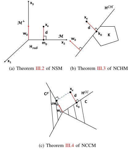
Fig. 2: An illustrative example of NCHM and NCCM in a 2D space.
1) Nearest convex hull method (NCHM): Nalbantov et
al. [15] propose the NCHM, which models each class as a
convex hull by using the training instances in that class. An illustrative example of NCHM is shown in a 2D space in
Fig. 2(a). The convex hulls of the two classes are shown as
the blue and red polygons, respectively. Since d1 < d2, we
assign xnew to class 1 in this example. In NCHM, we first
define convex hull as follows.
Definition II.2. Convex hull.LetS={xi}Ni=1be an arbitrary
set in a linear vector space. The convex hull, ch(S) ={z :
z =
N
P
i=1
αixi | xi ∈ S, 0 ≤ αi ≤ 1,
N
P
i=1
αi = 1}, is the
smallest convex set containingS. In other words,ch(S)is the
Given the training samples Xk ∈ RNk×p of class k, the
convex hull built by Xk is the set of vectors z ∈ Rp:
ch(Xk) = {z : z = XkTαCHk | 0 ≤ αCHk ≤
1, 1TαCHk = 1}, whereαCHk ∈RNk×1 is a vector containing
the coefficients associated with the Nk training samples in
Xk, 0 ≤ αCHk ≤ 1 means each element are in [0,1], and
1∈RNk×1 has all elements of one.
Given a new samplexnew∈R1×p, the distance fromxnew
to the convex hull ch(Xk)of thekth class is
dCHk = min
αCH
k
||xnew−(XTkαCHk )
T||
2,
s.t. 0≤αCHk ≤1, 1TαCHk = 1. (3)
Thenxnew is assigned to the class with the smallestdCHk :
ˆ
yCH= argmin
k
dCHk , (4)
whereyˆCH denotes the predicted label forxnew by NCHM.
2) Nearest convex cone method (NCCM): NCCM models each class as a convex cone by using the training instances in that class. We show an illustrative example of NCCM in a
2D space in Fig. 2(b). The convex cones for the two classes
are shown as the blue and red triangular area, respectively.
Since d1< d2, we assignxnew to class 1 in this example. In
NCCM, we first define convex polyhedral cone as follows.
Definition II.3. Convex polyhedral cone.A convex polyhedral cone is a convex cone that is generated by a finite number of
generators. Let S = {xi}Ni=1 be an arbitrary set in a linear
vector space. The set, cc(S) = {z : z =
N
P
i=1
αixi | xi ∈
S, αi≥0}, is the convex polyhedral cone generated byS.
Given the training samples Xk ∈ RNk×p of class k, the
convex polyhedral cone built by Xk is defined as a set of
vectors z ∈ Rp: cc(X
k) = {z : z =XTkαCCk | α
CC
k ≥0},
where αCCk ∈ RNk×1 and αCC
k ≥ 0 means each element in
αCCk is nonnegative. Thus each vector incc(Xk)is a conical
combination of the samples in Xk.
To assign a new samplexnew∈R1×pto one of the classes,
we calculate the distance fromxnew tocc(Xk):
dCCk = min
αCC
k
||xnew−(XTkαCCk )
T
||2, s.t. αCCk ≥0. (5)
Thenxnew is assigned to the class with the minimumdCCk :
ˆ
yCC = argmin
k
dCCk , (6)
whereyˆCC denotes the predicted label forxnew by NCCM.
III. DUAL ANALYSIS OF THE MINIMUM DISTANCE
PROBLEMS
Here we aim to establish a common platform to unify and compare the nearest-class-model methods through dual analysis of the minimum distance problems (1), (3) and (5). By studying the nearest-class-model methods together, we will have better understanding of the classification mechanisms of this important category of classification methods.
Dual analysis of the minimum distance problems enables us to find the separating hyperplanes, making finding the
minimum distance from a sample to a class model equivalent to finding the maximum distance from that sample to a separating hyperplane. Different from the Euclidean distances used in the previous section, we discuss more general cases in the normed linear vector space with arbitrary norm in this section. Examples and illustrations for the Hilbert space are also presented for a better geometric understanding.
We first introduce some important theoretical settings in preliminary. Then we show the dual analysis for the three minimum distance problems (1), (3) and (5). The dual analysis
for the subspace and the convex hull can be found in [25]
and we only show their results in Theorems III.2 and III.3,
respectively. In contrast, we provide a novel dual analysis and
its proof for the convex cone in Theorem III.4, based on the
relationship between a convex cone and its polar cone.
A. Preliminary
Definition III.1. Normed linear vector space.A normed linear
vector space is a vector space X, on which a real-valued
function is defined to map each element x in X into a real
number ||x|| called the norm of x. The norm satisfies the
following axioms: 1)||x|| ≥0 for allx∈ X,||x||= 0if and
only ifx= 0; 2)||x+y|| ≤ ||x||+||y||for eachx,y∈ X;
and 3)||αx||=|α|||x||for all scalarαand eachx∈ X.
Definition III.2. Linear functional. A transformation from a
vector space X into the space of real scalars is said to be a
functional onX. A functionalf on a vector spaceX is linear
if for any two vectors x,y ∈ X and any two scalars α, β
there holds f(αx+βy) =αf(x) +βf(y).
Definition III.3. The normed dual space. LetX be a normed linear vector space. The space of all bounded linear functionals
onX is called the normed dual ofX and is denoted by X∗.
The norm of an elementf ∈ X∗is||f||= sup
||x||≤1 |f(x)|.
Following [25], we usex∗ to denote the linear functionals
and writehx,x∗ito denotef(x).
Definition III.4. Real inner space. A real inner space is a
real linear vector space X together with an inner product,
which is a map from X × X to R and denoted by hx,yi
where x,y ∈ X. The inner product satisfies the following
axioms: 1) hx,yi=hy,xi; 2)hx+y,zi=hx,zi+hy,zi;
3) hλx,yi =λhx,yi; and 4)hx,xi ≥ 0; hx,xi= 0 if and
only ifxis the origin.
Definition III.5. Real Hilbert space. A complete real inner space is called a real Hilbert space.
A Hilbert space has the following nice property. If x∗
is a bounded linear functional on a Hilbert space H, there
exists a unique vector w ∈ H such that for all x ∈ H,
hx,x∗i=hx,wi. Moreover, we have||x∗||=||w||and every
w determines a unique bounded linear functional in this way.
B. Hyperplane
Definition III.6. Hyperplane. A hyperplane H in a linear
vector space X is a maximal proper linear variety, that is,
a linear variety H such that H 6=X, and if V is any linear
variety containing H, then eitherV =X or V =H.
Proposition 1 ( [25]). Let H be a hyperplane in a linear vector spaceX. Then there is a linear functionalx∗onX and a constant c such thatH ={x:hx,x∗i=c}. Conversely, if
x∗is a nonzero linear functional onX, the set{x:hx,x∗i= c} is a hyperplane in X. H is closed for everyc if and only if x∗ is continuous.
As shown in Proposition 1, hyperplanes have a close
rela-tionship with linear functionals. Thus the primal problem can be transformed to the dual problem by using the hyperplane as a media.
For a closed hyperplane H, we define two closed
half-spaces: the negative half-space {x : hx,x∗i ≤ c} and the
positive half-space {x : hx,x∗i ≥ c}. The distance from a
point to a hyperplane is of great importance in dual analysis,
thus we introduce it in TheoremIII.1.
Theorem III.1 ( [26]). Let xe be an element in a real
normed linear spaceX and letddenote its distance from the hyperplane H:{x:hx,x∗i=c}. Then,d= inf
h∈H ||xe−
h||=|hxe,x∗i−c|
||x∗|| .
C. Dual analysis for NSM, NCHM and NCCM
1) Dual analysis of the minimum distance problem in NSM:
In NSM, the separating hyperplane between an instancexeand
a subspace Mis found based on the orthogonal complement
M⊥ofM, which is stated in Theorem7. To make the
theoret-ical settings clear, we first define the orthogonal complement of a subspace as follows.
Definition III.7. Orthogonal complement.LetMbe a subset
of a normed linear spaceX. The orthogonal complementM⊥
of Mconsists of all elements x∗ ∈ X∗ orthogonal to every
vector in M.
Theorem III.2( [25]). Letxebe an element in a real normed
linear spaceX and letddenote its distance from the subspace
M. Suppose the orthogonal complement ofMisM⊥. Then,
d= inf
m∈M||xe−m||=||x∗||≤max1,x∗∈M⊥hxe,x
∗i, (7)
where the maximum on the right is achieved for some x∗0 ∈
M⊥.
If the infimum on the left is achieved for some m0 ∈ M,
thenx∗0 is aligned withxe−m0, i.e.hxe−m0,x∗0i=||xe−
m0||||x∗0||.
Based on Theorem III.1, the right-hand side of (7) can be
explained as the maximum distance fromxeto the hyperplane
Hsub ={x:hx,x∗i= 0 |x∗ ∈ M⊥}, since the maximum
is achieved when ||x∗|| = 1. Thus Theorem III.2 can be
understood as: The minimum distance from a point xeto the
subspace Mis equivalent to the maximum distance from xe
to the hyperplaneHsub.
For a better geometric understanding, we discuss
Theo-rem III.2 in the Hilbert space. For each x∗, we can find a
uniquew ∈ Hwhich is the normal vector of Hsub. Replace
x∗byw, the right-hand side of (7), i.e.hxe,wi, still denotes
the distance fromxetoHsub since the maximum is achieved
for||w||=||x∗||= 1. We also havehxe−m0,w0i=||xe−
m0||||w0||, thus xe−m0 =µw0 (µ >0). For any vector
m ∈ M, hxe−m0,mi =hµw0,mi=µhw0,mi= 0, as
w0∈ M⊥. This indicates thatxe−m0has the same direction
as w0 andxe−m0 is perpendicular to M.
x1
x2
x3
xe
m0
d
M
w0
M
Hsub
(a) TheoremIII.2of NSM
K k0
xe
d w0
HCH
(b) TheoremIII.3of NCHM
xe
c0
d w0
uw0
Cp
C HCC
[image:6.612.328.536.175.418.2](c) TheoremIII.4of NCCM
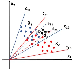
Fig. 3: Illustrative examples of (a) TheoremIII.2 of NSM,
(b) TheoremIII.3of NCHM and (c) Theorem III.4of
NCCM.
Fig.3(a) illustrates an example of TheoremIII.2. Suppose
x1,x2 andx3 are the orthogonal bases for R3. Assume M
is the subspace spanned by x2. Thus M⊥ is the subspace
spanned by x1 and x3. Suppose xe lies in the subspace
spanned by x2 and x3. Then the minimum distance from
xe to M is achieved at the point m0; and the maximum
distance fromxe to any subspaces with their normal vectors
inM⊥ is attained whenw
0has the same direction asx3; the
subspace associated with this maximum distance is denoted by
Hsub, which is a plane spanned byx1andx2, as illustrated in
Fig.3(a). That is, we can find that these two distances are the
same, both equal tod. The hyperplane with the normal vector
w0is actually the subspace spanned byx1andx2. The vector
xe−m0has the same direction asw0. This result is clear with
simple geometry, if we treatm0 as the orthogonal projection
of xe on the subspaceM.
2) Dual analysis of the minimum distance problem in NCHM: In NCHM, the maximum distance between xe and
a separating hyperplane that separates xe and a convex hull
Kis achieved when the separating hyperplane is a supporting
hyperplane ofK. The details are shown in Theorem8.
vector space X and let d > 0 denote its distance from the convex set K having support functional h, i.e. h(x∗) = supk∈Khk,x∗i. Then
d= inf
k∈K||xe−k||= max||x∗||≤1[hxe,x
∗i −h(x∗)], (8)
where the maximum on the right is achieved by somex∗0∈ X∗.
If the infimum on the left is achieved by some k0 ∈ K,
thenx∗0 is aligned with xe−k0, i.e.hxe−k0,x∗0i=||xe−
k0||||x∗0||.
The right-hand side of (8) can be understood as the
max-imum distance from xe to the hyperplane HCH = {x :
hx,x∗i = h(x∗)}. Thus Theorem III.3 indicates that the
minimum distance from xe to the convex hull is equivalent
to the maximum distance from xe to the hyperplaneHCH.
In the Hilbert space, we can find a unique w0∈ Hfor x∗0.
Since x∗0 is aligned with xe−k0, xe−k0 =µw0 (µ >0)
andxe−k0 has the same direction as w0.
Fig. 3(b) shows an intuitive example of Theorem III.3 in
R2. The minimum distance fromxetoKis achieved at point
k0, which lies on the nearest face of Ktoxe. The maximum
distance between xe and HCH that separates xe and K is
achieved when the nearest face of K to xe is inHCH. The
normal vectorw0 is perpendicular toHCH and has the same
direction asxe−k0.
3) Dual analysis of the minimum distance problem in NCCM: Inspired by the relationship between M and M⊥
used in Theorem III.2, we apply the relationship between a
convex cone and its polar cone to the dual analysis of (5) to
obtain the separating hyperplane for NCCM in TheoremIII.4.
We first introduce the definition of a polar cone and then show
Theorem III.4and its proof.
Definition III.8. Polar cone.Given a convex polyhedral cone
C in a normed space X, the set Cp={x∗∈ X∗:hx,x∗i ≤
0, ∀x∈C} is called the polar cone ofC.
Ifxeis an interior point ofC, thend= 0, which is a trivial
case. Thus in the following theorem, we discuss the case when
xe is not an interior point of C withd >0.
Theorem III.4. Letxebe an element in a real normed linear
spaceX. Letd >0denote the distance fromxeto the convex
cone C. Then,
d= inf
c∈C||xe−c||=||x∗||≤max1,x∗∈Cphxe,x
∗i,
where the maximum on the right is achieved for some x∗0 ∈
Cp.
If the infimum on the left is achieved for somec0∈C, then
x∗0is aligned withxe−c0, i.e.hxe−c0,x∗0i=||xe−c0||||x∗0||.
Proof. We first show that there exist somex∗∈Cp with the
hyperplane {x:hx,x∗i= 0} being able to separatexe and
C. The two closed half-spaces associated with the hyperplane
{x:hx,x∗i= 0} are {x:hx,x∗i ≥0} and{x:hx,x∗i ≤
0}. When x∗ ∈Cp,hc,x∗i ≤0 for c∈C, and C is in the
negative half-space. Since xe is not an interior point of C,
we can find some x∗ ∈ Cp such that hx
e,x∗i ≥ 0 and xe
is in the positive half-space. Thus xe and C lie in opposite
half-spaces determined by the hyperplane {x: hx,x∗i= 0}
withx∗∈Cp.
Let S() be the sphere centred at xe of radius . For
x∗ ∈ Cp having hx
e,x∗i ≥0 and ||x∗|| = 1, let ∗ be the
supremum of the’s for which the hyperplane{x:hx,x∗i=
0} separates C and S(). It is clear that 0 ≤ ∗ ≤d. Also
hxe,x∗i = ∗ when ||x∗|| = 1. Thus, for every x∗ ∈ Cp
having hxe,x∗i ≥0and||x∗||= 1, we have hxe,x∗i ≤d.
On the other hand, since C contains no interior point of
S(d), there is a hyperplane separating C and S(d), and thus
anx∗0∈Cp such thathxe,x∗i=d.
To prove the alignment statement, suppose c0 ∈ C and
||xe−c0|| = d. Since c0 ∈ C, hc0,x∗0i ≤ 0 and hxe−
c0,x∗0i ≥ hxe,x∗0i=d. However, according to the
Cauchy-Schwarz inequality, hxe−c0,x∗0i ≤ ||xe−c0||||x∗0|| = d.
Thushxe−c0,x∗0i=||xe−c0||||x∗0||=dandx∗0 is aligned
withxe−c0.
TheoremIII.4indicates that the minimum distance between
xe and C is equivalent to the maximum distance between
xe and the hyperplane HCC = {x : hx,x∗i = 0 | x∗ ∈
Cp,||x∗||= 1} that separatesxe andC.
In the Hilbert space, we can find a unique w0 ∈ H for
x∗0. Substitutingw0 withx∗0, we can get hxe,w0i=d. Also
hxe−c0,w0i=||xe−c0||||w0||=d. The equality holds when
xe−c0=µw0 (µ >0). Thus we can get the following two
conclusions. First,hc0,w0i= 0, which indicates that c0 and
w0 are orthogonal. Second,xe=c0+µw0, which indicates
that xe can be decomposed toc0∈C and µw∈Cp. These
two conclusions indicates that the orthogonal decompositions
ofxetoCandCparec0andµw0, respectively. Based on the
Moreau’s theorem in the Hilbert space [27],c0andµw∈Cp
are the projections ofxe onC andCp, respectively.
Fig. 3(c) illustrates Theorem III.4 in R2. The minimum
distance d from xe to C is achieved by c0, which is the
orthogonal projection of xe to the nearest face of C to xe.
The maximum distance from xe to HCC is achieved when
HCC contains the nearest face of C toxe. It is obvious that
the distance fromxeto thisHCC is alsod. The normal vector
associated with this hyperplane is w0, which has the same
direction asxe−c0; the pointµw0is the orthogonal projection
of xe toCp.
IV. UNIFY THE NEAREST-CLASS-MODEL METHODS
In Section IV-A, we propose the novel separating
hyper-plane classification (SHC) framework based on the theoretical
discussion in Section III. The nearest-class-model methods
can be unified under the SHC framework with different set
of constraints on the normal vectorsw and the bias b.
The SHC framework has two advantages. First, we can explain the empirical classification performance by analysing the discriminative abilities of the normal vectors. Second, we can design new nearest-class-model methods by imposing appropriate constraints to the framework based on the prop-erties of the data. We show an example of designing a new soft NCCM classifier under the SHC framework, to solve the
A. A novel separating hyperplane classification (SHC) frame-work
xnew
d1 d2
X1 X
2
H1 H2
Fig. 4: The separating hyperplane classification framework.
The dual analysis enables us to explain the classification schemes of NSM, NCCM and NCHM from the separating
hyperplane point of view. Theorems III.2, III.3 and III.4
indicate that the three methods all classify a test sample by using separating hyperplanes associated with each class. We
illustrate a binary classification case in Fig. 4. The red and
blue ellipses represent the two class models, respectively, and the red and blue lines represent the separating hyperplanes
between a new instance xnew and the class models,
respec-tively.xnew is classified by comparing its distance to the two
separating hyperplanes.
Based on the separating hyperplanes, we can derive a new separating hyperplane classification (SHC) framework for different class representation models and distances with
arbitrary norms: First, for thekth class, we obtain
max
ck,||x∗k||=1
dk=hxnew,x∗ki −ck
s.t. constraint(x∗k, ck), (9)
wherex∗
k andck are the two parameters to define the
separat-ing hyperplane Hk ={x:hx,x∗ki=ck} betweenxnew and
thekth class model, and constraint(x∗k, ck)denotes constraints
onx∗k andck. Then,xnew is assigned to the classkwith the
minimum dk.
This SHC framework for two-class classification can be explained as follows. For each test sample, we find a pair of separating hyperplanes that separate the test sample and the two class models, respectively. The test sample is then assigned to the class with the minimum distance from that sample to the corresponding hyperplane.
In the SHC framework, the normal vectors of the sep-arating hyperplanes play important roles in classification.
TheoremsIII.2,III.3andIII.4suggest that the dual functionx∗0
that determines the separating hyperplane is aligned with the
vectorxnew−x0, wherex0is the nearest point toxnewin the
class model. In the Hilbert space, this means that the normal
vector of the separating hyperplane is parallel withxnew−x0.
The norm of xnew −x0 is defined as the distance from
xnew to the class model. Thus the discriminative information
contained in the direction of xnew−x0, which is also the
direction of the associated normal vector of the hyperplane, is vital to classification. The more the discriminative information
contained in the normal vector, the higher the classification ac-curacy. In other words, to get better classification, constraints should be specified to make the normal vector contain more discriminative information.
In NSM, NCHM and NCCM, the Euclidean norm|| · ||2 is
used. We summarise constraint(x∗k, ck)for NSM, NCHM and
NCCM in TableI. Note thatx∗k is replaced bywk. For NSM,
wk has a closed-form solution of xc,knew −xc,knewPk, where
xc,k
[image:8.612.133.215.109.200.2]new is the centredxnewby the column mean ofXk.
TABLE I: constraint(x∗k, ck)for NSM, NCHM and NCCM.
NSM NCHM NCCM
hxc,knewPk,wki= 0 hxnew,wki ≥ck hxnew,wki ≥0
ck= 0 hxki,wki ≤ck hxki,wki ≤0
ck= 0
Pkdenotes the projection matrix for classk.
xk i ∈R1
×pdenotes theith row inXk.
B. A novel soft nearest-convex-cone method (soft NCCM)
Besides the constraints listed in Table I, other constraints
can also be specified based on the properties of the dataset and the requirements from the user, to extend further. In this section, we show an example of designing a new nearest-class-model method under the SHC framework, to better classify data with overlapping class models.
x1 x2
X1
X2 xnew
d2 d1 c11
c12 c21
c22 s12
[image:8.612.377.493.378.489.2]s21
Fig. 5: An illustrative example of soft NCCM in a 2D space.
When the class models overlap, the class memberships of the test instances locating in the overlapping area are am-biguous and cannot be determined by the nearest-class-model methods. This is because the distances from those instances to class models are all zeros and we cannot find a hyperplane to separate them with the class models. We illustrate this situation
in Fig. 5. The original convex cone models are shown by the
triangular areas constructed by the solid lines: the blue solid
linesc11andc12form the convex cone for the first class while
the red solid lines c21 and c22 form the convex cone for the
second class. We can observe a large overlapping area between
the two convex cones. The instances located betweenc21 and
c12 cannot be clearly classified to a specific class because of
the overlapping problem.
To address this problem, we propose a novel nearest-class-model method, the soft NCCM classifier, by imposing
proper constraints into the optimisation problem (9). In Fig.5,
by using the soft NCCM, we expect to get two separating
the first class and the second class, respectively. It is clear that we actually reduce the areas of the convex cones by
pushing the overlapping boundariesc12andc21towardsxnew
and obtain the new boundaries s12 ands21, respectively. The
resulting ‘soft’ convex cones of the two classes are constructed
by the blue lines c11 and s12 for the first class and the red
lines c22 and s21 for the second class. Thus xnew can be
then classified by comparing d1 andd2 to the two separating
hyperplanes s12 ands21, respectively.
In soft NCCM, we design the constraints to achieve the following two aims: first, the test instances in the overlap-ping area can be classified unambiguously, and second, the discriminative between-class information is utilised to make separating hyperplanes better for classification. The optimisa-tion problem is written as follows:
max
||wk||2=1
dSCCk =wTkxnew,
s.t. wTkxnew≥0,
wTkxki ≤ξi, i= 1,2, . . . , Nk,
wTkx−jk≥ −ξj, j= 1,2, . . . , N−k,
ξi≥0∀i, ξj≥0∀j,
X
i
ξi+
X
j
ξj ≤C, (10)
where the subscript kdenotes thekth class while −kdenotes
all other classes, i.e. Nk is the number of training samples in
the kth class and N−k is the number of training samples in
all classes except for the kth class.
To achieve the first aim, we introduce slack variables ξi,
allowing some of the training instances from the kth class
to locate on the same side of the separating hyperplane as
xnew. In this way, we can find a hyperplane that can separate
xnewand the convex cone class model with tolerance of errors,
even whenxnew locates in the convex cone. Thus there is no
overlapping area when we use the separating hyperplanes to
classifyxnew, and an unambiguous class membership can be
obtained. To achieve the second aim, we propose the third constraint which utilises the discriminative information from
other classes and makes the training instances from the kth
class and those from all other classes locate on different sides
of the separating hyperplane corresponding to the kth class.
V. EXPERIMENTS
For illustration, we apply NSM, NCHM, NCCM and soft NCCM to two types of high-dimensional data, the
spectro-scopic data and the face image data, in SectionsV-AandV-B,
respectively. For each type of data, we first show the classi-fication results of the four nearest-class-model methods. The classification performances of a popular classification method for high-dimensional data, support vector machine (SVM), are also recorded to show the effectiveness of the nearest-class-model methods. We then analyse why a class nearest-class-model performs better than others, by exploring the discriminative abilities of the normal vectors based on the SHC framework.
A. The spectroscopic data
10 20 30 40 50 60 70 80 90 100 2
2.5 3 3.5 4 4.5 5 5.5 6
Wavelengths
Abundance
Less than 20% More than 20%
(a) The fat dataset
100 200 300 400 500 600 700 800 9001000 0.7
0.8 0.9 1 1.1 1.2 1.3 1.4 1.5 1.6 1.7
Wavelengths
1/log(reflectance)
Chicken samples Turkey samples
[image:9.612.323.554.65.171.2](b) The meat dataset
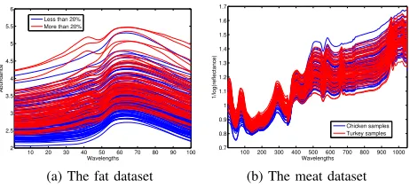
Fig. 6: The spectroscopic datasets.
1) Datasets: We use two high-dimensional spectroscopic datasets, the fat dataset and the meat dataset, in the following experiments.
The fat dataset [28] measures the spectra of finely chopped
meat, which can be downloaded from http://lib.stat.cmu.edu/
datasets/tecator. Each spectrum is measured at 100 wave-lengths. The dataset contains 193 spectra, with 122 meat samples of less than 20% fat and 71 samples of larger than
20% fat. Fig.6(a)shows the spectra of the fat dataset.
For the fat dataset, a training set contains 100 randomly selected samples, with 35 samples of less than 20% fat and 35 samples of larger than 20% fat, and a test set contains the remaining samples.
The meat dataset contains 55 chicken and 54 turkey meat spectra measured at 1051 wavelengths. We use the first 350 wavelengths ranging from 400 to 1100 nm, following the
suggestion in Arnalds et al. [29]. Fig.6(b)shows the spectra
of the meat dataset.
For the meat dataset, a training set contains 27 chicken samples and 27 turkey samples, and a test set contains 28 chicken samples and 27 turkey samples.
2) Experiment settings: In NSM, the dimensions of the two class subspaces are tuned by 10-fold cross-validation on the training set. The dimensions are chosen to minimise the classification error. In NCHM, the optimisation prob-lem (3) is solved using the ‘cvx’ package in MATLAB. In NCCM, the optimisation problem (5) is solved using the ‘lsqnonneg’ function in MATLAB. In soft NCCM, the
optimisation problem (10) and the parameter C is tuned by
10-fold cross-validation from[10−1,1,10]. In SVM, the linear
kernel is adopted, because it is usually recommended for
high-dimensional data [30]. We randomly split the data to a training
set and a test set 100 times and the experiments are performed on all training/test splits. The classification accuracies of all the experiments are recorded and depicted in boxplots.
3) Classification results: The classification accuracies of SVM, NSM, NCHM, NCCM and soft NCCM for the two
datasets are shown in Fig. 7. It is clear that soft NCCM can
SVM NSM NCHM NCCM Soft NCCM
Classification accuracy
0.84 0.86 0.88 0.9 0.92 0.94 0.96 0.98 1
(a) The fat dataset
SVM NSM NCHM NCCM Soft NCCM
Classification accuracy
0.3 0.4 0.5 0.6 0.7 0.8 0.9 1
[image:10.612.62.293.65.165.2](b) The meat dataset
Fig. 7: The classification accuracies of SVM, NSM, NCHM, NCCM and soft NCCM on the two spectroscopic datasets.
the effectiveness of the constraints that we propose in (10). For the fat data, SVM and soft NCCM have the best median accuracies. However, it is obvious that soft NCCM has a much smaller variance in classification accuracies than SVM. The classification performances of NSM, NCHM are worse than that of NCCM, which suggests that convex cone is a better class model than PC subspace and convex hull for this dataset. For the meat data, SVM performs the worst with a large variation. Soft NCCM has a similar median to NSM while less extreme low accuracies than NSM. Comparing the clas-sification performances of NSM, NCHM and NCCM, we can state that PC subspace is a better class model for this dataset compared with the geometric class models.
w
20 40 60 80
Discriminative ability
0 0.1 0.2 0.3 0.4 0.5 0.6 0.7 0.8 0.9 1
wS
wCH
wCC
wSCC
(a) Fat: less than 20%
w
20 40 60 80
Discriminative ability
0 0.1 0.2 0.3 0.4 0.5 0.6 0.7 0.8 0.9 1
wS
wCH
wCC
wSCC
(b) Fat: more than 20%
w
10 20 30 40 50
Discriminative ability
0 0.1 0.2 0.3 0.4 0.5 0.6 0.7 0.8 0.9 1
wS
wCH
wCC
wSCC
(c) Meat: chicken
w
10 20 30 40 50
Discriminative ability
0 0.1 0.2 0.3 0.4 0.5 0.6 0.7 0.8 0.9 1
wS
wCH
wCC
wSCC
[image:10.612.60.289.392.610.2](d) Meat: turkey
Fig. 8: The discriminative abilities, denoted by wS,wCH,
wCC andwSCC, of the normal vectors of NSM, NCHM,
NCCM and soft NCCM, respectively, for the two spectroscopic datasets.
4) Analysis of classification results: Section V-A3 shows that different data prefer different class models. To understand this pattern, we compare the normal vectors of pairs of separating hyperplanes of the four methods. As discussed in
SectionIV-A, the more discriminative the normal vectors are,
the higher the classification accuracy.
Here we measure the discriminative ability of the normal vectors by the classification accuracies of linear discriminant analysis (LDA). More specifically, for each test instance, we have two normal vectors associated with the two separating hyperplanes for the two classes, respectively. We project all the instances to each normal vector and apply LDA on the projected instances based on 100 random training/test splits. The mean classification accuracies are recorded for the two normal vectors. We repeat this procedure for all test instances from one training/test split in the previous section.
We show in Fig.8the mean classification accuracies for the
normal vectors of NSM, NCHM, NCCM and soft NCCM,wS,
wCH,wCCandwSCC. The horizontal line indices the normal
vectors for the test instances and the vertical line denotes the discriminative abilities. The black solid line shows the classification accuracy of 0.5, which is a threshold indicating with and without discriminative ability.
Obviously, the normal vectors of soft NCCM, wSCC, has
the best discriminative abilities with the highest curves for both classes and both datasets, which is consistent with its best classification performances on the two datasets. For
the fat data, wS of NSM has much lower discriminative
abilities in most cases, which is also consistent with its worst classification performance compared with other methods. For the meat data, NSM has better classification performance than NCHM and NCCM and this is also shown in the turkey meat
class in Fig.8(d):wS has a higher curve thanwCHandwCC.
B. The face image data
1) Dataset: To further show the effectiveness of the pro-posed SHC framework and the new soft NCCM, we also apply the methods to another popular type of high-dimensional data, the face image data. We use the extended Yale face
database B [11] as an exemplar. The database contains 38
individuals, each with around 64 near frontal images under different illuminations. Each image has a frontal face cropped
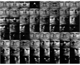
from the original image and is resized to 32×32 pixels. Fig.9
shows the 64 face images of one individual. Here we take the first ten individuals in the experiments for illustration.
Fig. 9: Example face images in the Yale face database B.
[image:10.612.373.502.544.649.2]SVM NSM NCHM NCCM Soft NCCM
Classification accuracy
[image:11.612.322.552.61.290.2]0.88 0.9 0.92 0.94 0.96 0.98
Fig. 10: The classification accuracies of SVM, NSM, NCHM, NCCM and soft NCCM on the face image data.
3) Classification results: Fig. 10 shows the boxplots for the classification accuracies of the five classifiers. All methods have median accuracies over 0.9, which shows their effective-ness to classify face image data. NSM has the lowest box and the largest variation among all methods. SVM is competitive with NCHM, while NCHM has a higher median accuracy.
The two cone-based methods, NCCM and soft NCCM, show the best classification accuracies. This is reasonable because the frontal face images under various illumination conditions
can be effectively represented by an illumination cone [11].
Soft NCCM performs even better than NCCM, which shows the advantage of considering the between-class information.
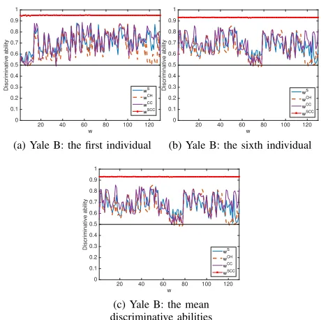
4) Analysis of classification results: To show the discrim-inative ability of the normal vector, we make a slight change to the multi-class case here compared with the binary case in the spectroscopic data. We first project all the data to the direction of the normal vector and then apply LDA to do binary classification: one is for the class associated with that normal vector and the other is for other classes. Given one normal vector, we repeat this process nine times for all other nine classes and take the average of the mean classification accuracies as the discriminative ability of that normal vector. The reason for this is that, based on the separating hyperplane corresponding to one class, it is hard to achieve multi-class classification. It is natural to use this separating hyperplane to distinguish between the corresponding class and the other classes. All other settings to analyse the classification results are the same as those for the spectroscopic data.
For the ten classes tested in the experiments, we can find the
discriminative abilities of the ten normal vectors. Figs. 11(a)
and 11(b) show the discriminative abilities of the normal
vectors corresponding to the first and sixth individuals in one training/test split, respectively, for example. The normal vectors of soft NCCM have the highest discriminative abilities.
We can also observe that the curves forwCCare slightly above
those forwSandwCHin most cases. To visualise the ten plots
together, we also plot the means of the discriminative abilities
of the ten normal vectors in Fig.11(c). The pattern is roughly
the same as that in Figs. 11(a)and11(b).
To sum up, we can draw two conclusions from the exper-iments on both the high-dimensional spectroscopic and face image datasets. First, the new soft NCCM that solves the overlapping class model problem has the best classification performances over all compared methods. Second, the discrim-inative ability of the normal vector is associated with the
clas-w
20 40 60 80 100 120
Discriminative ability
0 0.1 0.2 0.3 0.4 0.5 0.6 0.7 0.8 0.9 1
wS
wCH
wCC
wSCC
(a) Yale B: the first individual
w
20 40 60 80 100 120
Discriminative ability
0 0.1 0.2 0.3 0.4 0.5 0.6 0.7 0.8 0.9 1
wS
wCH
wCC
wSCC
(b) Yale B: the sixth individual
w
20 40 60 80 100 120
Discriminative ability
0 0.1 0.2 0.3 0.4 0.5 0.6 0.7 0.8 0.9 1
wS
wCH
wCC
wSCC
[image:11.612.115.240.62.157.2](c) Yale B: the mean discriminative abilities
Fig. 11: The discriminative abilities of two normal vectors and the mean discriminative abilities of NSM, NCHM,
NCCM and soft NCCM for the Yale face database B.
sification performance of nearest-class-model methods, which demonstrates the effectiveness of the new SHC framework in explaining the classification results.
VI. CONCLUSIONS AND FUTURE WORK
In this paper, we establish a new separating hyperplane classification (SHC) framework to unify three nearest-class-model methods for high-dimensional data: NSM, NCHM and NCCM. The SHC framework is established on the theoretical results from the dual analysis of the three methods. We show a new theorem for the dual analysis of NCCM by discovering the relationship between a convex cone and its polar cone.
Based on this novel SHC framework, we can explain why one class model is good to classify a specific dataset by showing the discriminative ability of the normal vectors of the separating hyperplanes. The higher the discriminative abilities of the normal vectors, the higher the classification accuracy of one method. The experiment results also demonstrate this argument. In addition, we propose a new soft NCCM under the SHC framework to solve the overlapping class model problem. The experiments on both spectroscopic data and face image data show the superior classification performance of the new soft NCCM over other nearest-class-model methods.
Our future work includes: 1) investigating and unifying
more class models, such as the affine hull [31] and
hyper-disk [17], [32] class models; 2) unifying the
ACKNOWLEDGEMENTS
We sincerely thank the four anonymous reviewers for their insightful and critical comments, which largely improved the theoretical and empirical presentations of our work, and stimulated our proposal of soft NCCM.
REFERENCES
[1] S. Wold, “Pattern recognition by means of disjoint principal components models,”Pattern Recognition, vol. 8, no. 3, pp. 127–139, 1976. [2] P. Poˇr´ızka, J. Klus, A. Hrdliˇcka, J. Vr´abel, P. ˇSkarkov´a, D. Prochazka,
J. Novotn`y, K. Novotn`y, and J. Kaiser, “Impact of laser-induced break-down spectroscopy data normalization on multivariate classification accuracy,”Journal of Analytical Atomic Spectrometry, vol. 32, no. 2, pp. 277–288, 2017.
[3] Y. Lee, S.-H. Han, and S.-H. Nam, “Soft independent modeling of class analogy (SIMCA) modeling of laser-induced plasma emission spectra of edible salts for accurate classification,” Applied Spectroscopy, p. 0003702817697337, 2017.
[4] K. N. Basri, M. N. Hussain, J. Bakar, Z. Sharif, M. F. A. Khir, and A. S. Zoolfakar, “Classification and quantification of palm oil adulteration via portable NIR spectroscopy,”Spectrochimica Acta Part A: Molecular and Biomolecular Spectroscopy, vol. 173, pp. 335–342, 2017.
[5] R. Zhu and J.-H. Xue, “On the orthogonal distance to class subspaces for high-dimensional data classification,”Information Sciences, vol. 417, pp. 262 – 273, 2017.
[6] R. Zhu, K. Fukui, and J.-H. Xue, “Building a discriminatively ordered subspace on the generating matrix to classify high-dimensional spectral data,”Information Sciences, vol. 382–383, pp. 1–14, 2017.
[7] O. Yamaguchi, K. Fukui, and K.-i. Maeda, “Face recognition using tem-poral image sequence,” inProceedings of the Third IEEE International Conference on Automatic Face and Gesture Recognition. IEEE, 1998, pp. 318–323.
[8] K. Fukui and O. Yamaguchi, “Face recognition using multi-viewpoint patterns for robot vision,” inThe Eleventh International Symposium on Robotics Research. Springer, 2005, pp. 192–201.
[9] M. Nishiyama, O. Yamaguchi, and K. Fukui, “Face recognition with the multiple constrained mutual subspace method,” in International Conference on Audio-and Video-Based Biometric Person Authentication. Springer, 2005, pp. 71–80.
[10] K. Fukui and A. Maki, “Difference subspace and its generalization for subspace-based methods,”IEEE Transactions on Pattern Analysis and Machine Intelligence, vol. 37, no. 11, pp. 2164–2177, 2015.
[11] K.-C. Lee, J. Ho, and D. J. Kriegman, “Acquiring linear subspaces for face recognition under variable lighting,”IEEE Transactions on Pattern Analysis & Machine Intelligence, no. 5, pp. 684–698, 2005.
[12] Y. Chi, “Nearest subspace classification with missing data,” inSignals, Systems and Computers, 2013 Asilomar Conference on. IEEE, 2013, pp. 1667–1671.
[13] Y. Chi and F. Porikli, “Connecting the dots in multi-class classification: From nearest subspace to collaborative representation,” in Computer Vision and Pattern Recognition (CVPR), 2012 IEEE Conference on. IEEE, 2012, pp. 3602–3609.
[14] C.-P. Chen and C.-S. Chen, “Intrinsic illumination subspace for lighting insensitive face recognition,”IEEE Transactions on Systems, Man, and Cybernetics, Part B (Cybernetics), vol. 42, no. 2, pp. 422–433, 2012. [15] G. Nalbantov, P. Groenen, and C. Bioch, “Nearest convex hull
classifi-cation,” Erasmus University Rotterdam, Erasmus School of Economics (ESE), Econometric Institute, Tech. Rep., 2006.
[16] H. Cevikalp and B. Triggs, “Face recognition based on image sets,” in
IEEE Conference on Computer Vision and Pattern Recognition (CVPR). IEEE, 2010, pp. 2567–2573.
[17] H. Cevikalp, B. Triggs, and R. Polikar, “Nearest hyperdisk methods for high-dimensional classification,” inICML. ACM, 2008, pp. 120–127. [18] X. Zhou and Y. Shi, “Nearest neighbor convex hull classification method for face recognition,” in International Conference on Computational Science. Springer, 2009, pp. 570–577.
[19] D. Fern´andez-Francos, ´O. Fontenla-Romero, and A. Alonso-Betanzos, “One-class convex hull-based algorithm for classification in distributed environments,”IEEE Transactions on Systems, Man, and Cybernetics: Systems, 2017.
[20] T. Kobayashi and N. Otsu, “Cone-restricted subspace methods,” in19th International Conference on Pattern Recognition (ICPR 2008). IEEE, 2008, pp. 1–4.
[21] M. S. Bazaraa, H. D. Sherali, and C. M. Shetty,Nonlinear programming: theory and algorithms. John Wiley & Sons, 2013.
[22] H. Cevikalp, “Best fitting hyperplanes for classification,”IEEE Trans-actions on Pattern Analysis and Machine Intelligence, 2016.
[23] O. L. Mangasarian and E. W. Wild, “Multisurface proximal support vector machine classification via generalized eigenvalues,”IEEE Trans-actions on Pattern Analysis and Machine Intelligence, vol. 28, no. 1, pp. 69–74, 2006.
[24] Jayadeva, R. Khemchandani, and S. Chandra, “Twin support vector machines for pattern classification,” IEEE Transactions on Pattern Analysis and Machine Intelligence, vol. 29, no. 5, pp. 905–910, 2007. [25] D. G. Luenberger,Optimization by Vector Space Methods. John Wiley
& Sons, 1969.
[26] D. Zhou, B. Xiao, H. Zhou, and R. Dai, “Global geometry of SVM classifiers,” Technical Report 30-5-02, Institute of Automation, Chinese Academy of Sciences, Tech. Rep., 2002.
[27] J.-J. Moreau, “D´ecomposition orthogonale dun espace hilbertien selon deux cˆones mutuellement polaires,”CR Acad. Sci. Paris, vol. 255, pp. 238–240, 1962.
[28] F. Ferraty and P. Vieu,Nonparametric Functional Data Analysis: Theory and Practice. Springer Science & Business Media, 2006.
[29] T. Arnalds, J. McElhinney, T. Fearn, and G. Downey, “A hierarchical discriminant analysis for species identification in raw meat by visible and near infrared spectroscopy,”Journal of Near Infrared Spectroscopy, vol. 12, no. 3, pp. 183–188, 2004.
[30] C.-W. Hsu, C.-C. Chang, and C.-J. Lin, “A practical guide to support vector classification,” 2003.
[31] H. Cevikalp, B. Triggs, H. S. Yavuz, Y. K¨uc¸¨uk, M. K¨uc¸¨uk, and A. Barkana, “Large margin classifiers based on affine hulls,” Neuro-computing, vol. 73, no. 16, pp. 3160–3168, 2010.
[32] H. Cevikalp and B. Triggs, “Hyperdisk based large margin classifier,”
Pattern Recognition, vol. 46, no. 6, pp. 1523–1531, 2013.
Rui Zhureceived her Ph.D. degree in statistics from University College London in 2017. She is a lecturer in the Faculty of Actuarial Science and Insurance, City, University of London. Her research interests include spectral data analysis, hyperspectral image analysis, subspace-based classification methods and image quality assessment.
Ziyu Wangreceived her Ph.D. degree in the security science and statistical science from University Col-lege London in 2017. Her research interests include hyperspectral image analysis, sparse representation and statistical classification.
Naoya Sogi received his B.E. and M.E. degrees from the University of Tsukuba in 2017 and 2019, respectively. He is currently a Ph.D. candidate at the University of Tsukuba. His interests include the theories of computer vision, pattern recognition, machine learning and applications of these theories.
Kazuhiro Fukui received his Ph.D. degree from Tokyo Institute of Technology in 2003. He is a professor in the Department of Computer Science, University of Tsukuba. His interests include the theories of computer vision, pattern recognition, and applications of these theories. He has been serving as a program committee member at many pattern recog-nition and computer vision conferences, including as an Area Chair of ICPR’12, 14 and 16.