Measuring smoothness of real-valued functions defined by sample points on the unit circle

Measuring Smoothness of Real-Valued Functions

Defined by Sample Points on the Unit Circle

Stephan Weiss

, Ian K. Proudler

, and Malcolm D. Macleod

1_{Dept. Electronic & Electrical Engineering, University of Strathclyde, Glasgow G1 XW, Scotland}

2 _{QinetiQ Ltd., Malvern, Hertfordshire, UK}

{stephan.weiss,ian.proudler,malcolm.macleod}@strath.ac.uk

Abstract—In the context of extracting analytic eigen- or singu-lar values from a polynomial matrix, a suitable cost function is the smoothness of continuous, real, and potentially symmetric periodic functions. This smoothness can be measured as the power of the derivatives of that function, and can be tied to a set of sample points on the unit circle that may be incomplete. We have previously explored the utility of this cost function, and here provide refinements by (i) analysing properties of the cost function and (ii) imposing additional constraints on its evaluation.

I. INTRODUCTION

For a matrix R(z) :_C →_CM×M _{that comprises rational}

analytic functions in the variablez ∈C and is parahermitian such that RP(z) = RH(1/z∗) = R(z) [1], a parahermitian matrix eigenvalue decomposition (EVD) with analytic factors exists in almost all cases [2], [3]. These may generally be transcendental functions and as such absolutely conver-gent Laurent series. If the decomposition is approximated by Laurent polynomials, the choice for the factors widens, and include others, such as spectrally majorised solutions, which time domain polynomial matrix EVD algorithms [4]– [8] encourage or even guarantee [9] to obtain. The difference between these solutions is contrasted in Fig. 1. In comparison, discrete Fourier transform (DFT) domain algorithms [10]– [13] can permit a choice to extract approximations of both spectrally majorised and analytic solutions.

DFT-domain algorithms do not naturally possess the fre-quency domain coherence that has motivated time domain ap-proaches [4], [5], [7], and therefore require association across frequency bins. In [10]–[12] this association is based on the continuity of eigenvectors, which in principle is easier to detect than a non-differentiability of eigenvalues. The association de-cisions are most crucial nearQ-fold algebraic multiplicities of eigenvalues, where eigenvectors can be arbitrarily selected as an orthogonal basis within aQ-dimensional subspace [2], thus creating challenges for an eigenvector-driven association [13]. Similar challenges exist for the analytic SVD [14]–[18], where analytic singular values can be extracted for a matrix

A(ω), ω ∈ _R, over a given interval of ω, i.e. A(ω) is not considered to be periodic inω, and hence does not correspond to a discrete time function. In fact, in [15],ωis not necessarily This work was supported by the Engineering and Physical Sciences Research Council (EPSRC) Grant number EP/S000631/1 and the MOD University Defence Research Collaboration in Signal Processing.

a frequency parameter. The extraction of analytic functions in A(ω) is driven by their arc length as a measure for smoothness [15] or by a Chebyshev interpolation. For a self-adjoint matrix A(ω) (equivalent to parahermitianity on the unit circle), an analytic EVD according to Rellich exists [19], and again an algorithm for their extraction requires a suitable cost function.

Since analyticity implies infinite differentiability, in this paper we explore a suitable cost function that can distin-guish between analytic and alternative (such as spectrally majorised) solutions: the power of derivatives of a function

F(ejΩ_{). In [20], we have explored this metric and successfully}

applied it to drive an analytic eigenvalue extraction in [13]. The extraction algorithm in [13] aims to create associations for maximally smooth functions from an initially small but iteratively increasing number of sample points, similar to the ‘missing samples problem’ [21]. Any yet unassigned sample points are chosen such that a maximally smooth function for the given sample set is extracted.

In this paper, we aim to further explore the smoothness metric in [20], establish that is positive real, and introduce additional constraints onto the solution to reflect the real-valued and potentially symmetric nature of the eigenvalues of a parahermitian matrix [2]. For this, Sec. II illuminates the problem, with the interpolation of a continuous function based on samples points discussed in Sec. III. Its derivative powers are tied to the sample points in Sec. IV, followed by a

0 /4 /2 3 /4 5 /4 3 /2 7 /4 2

0 2 4

(a)

0 /4 /2 3 /4 5 /4 3 /2 7 /4 2

0 2 4

(b)

0 /4 /2 3 /4 5 /4 3 /2 7 /4 2 0

2 4

(2)

(2) (a)

0 /4 /2 3 /4 5 /4 3 /2 7 /4 2 0

2 4

(b)

0 /4 /2 3 /4 5 /4 3 /2 7 /4 2 0

2 4

(c)

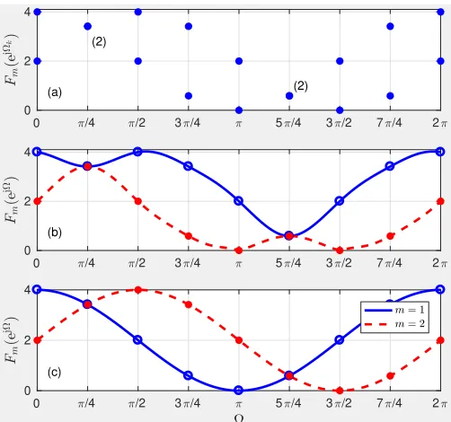
Fig. 2. (a) set of sample points forK= 8andM= 2, and (b) spectrally majorised and (c) analytic associations of values and their interpolations.

smoothness metric for an incomplete grid of sample points is elaborated in Secs. V and VI. Finally some results and conclusions are provided in Secs. VII and VIII.

II. PROBLEMFORMULATION

We are given a set of M K sample points, which is spread over K out of a total of N frequency bins and contains M

values per bin. The ultimate aim is to find an association of this set to M functions that interpolate across the distinct sample points as smoothly as possible. As an example, Fig. 2 demonstrates this for a case of N = K = 8 and M = 2. The sample points are drawn in Fig. 2(a), whereby algebraic multiplicities of values greater than one are indicated in parentheses. Two different associations and their interpolation — to be discussed later — are shown in Fig. 2(b) and (c).

Thus, the challenge is to measure the smoothness of a function F(ejΩ_{) defined by sample points F}

k = F(ejΩk) on

a regular grid ofN frequency binsΩk = 2πk/N. We further

specify:

(C1) onlyK≤N sample points may be known, (C2) F(ejΩ_{)is real-valued,}

(C3) F(ejΩ_{)may be symmetric with respect toΩ = 0.}

As a result, we can state for its inverse Fourier transformf[τ],

f[τ] = 1 2π

Z π

−π

F(ejΩ)ejΩτdΩ, (1) or in short f[τ]◦—•F(ejΩ_{), that f[τ] must be symmetric}

such that f[τ] =f∗[−τ]and that it may be real valued. III. DIRICHLETINTERPOLATION

For f[τ] to be a symmetric sequence, it has to be of even order, or odd length. However, to align with powerful fast Fourier transform techniques, it can be advantageous to select

the number of sample pointsNif not to be a power of two then at the very least to be even. We first address the simple case ofN being odd, and thereafter focus on the more challenging case of N being even.

A. Interpolation for Odd Number of Sample Points

ForN being odd, the interpolation across the sample points

Fk can be accomplished by the Dirichlet kernelPN(ejΩ),

PN(ejΩ) =

sin N₂Ω

sin 1₂Ω =

(N−1)/2

X

τ=−(N−1)/2

e−jΩτ , (2)

which links to a rectangular window pN[τ] that sits centred

with respect toτ = 0.

The kernel in (2) permits to express a2π-periodic function

F(ejΩ) as a superposition of weighted and shifted contribu-tions,

F(ejΩ) = 1

N

N−1

X

k=0

FkPN(ej(Ω−Ωk)) (3)

= 1

N

N−1

X

k=0

Fk

(N−1)/2

X

τ=−(N−1)/2

e−j(Ω−Ωk)τ _{, (4)}

=

(N−1)/2

X

τ=−(N−1)/2

f[τ]e−jΩτ , (5)

where (4) utilises the Fourier series representation of the kernel, and f[τ] is the result of an N-point inverse discrete Fourier transform (IDFT) of F(ejΩk_{). The outcome in (5)}

confirmsf[τ]◦—•F(ejΩ_{), as set out in (1).}

B. Interpolation for Even Number of Sample Points

The challenge for even N is exemplified in Fig. 3. When basing an inverse Fourier transform on the discrete spectrum represented by the sample points Fk of F(ejΩ), a periodised

time domain f˜[τ]◦—•F(ejΩk_{)emerges. For an odd number}

of samples pointsFk, here N = 3, in Fig. 3(a), f[τ] can be

extracted as the fundamental period of f˜[τ] in Fig. 3(b). In the even case in Fig. 3(c) and (d), f˜[τ] will be periodic with

N, but also needs to be symmetric. Without loss of generality,

F(ejΩk₎

Ω

0

-2π 2π

~

f[τ]

0 -1

-2 1 2

(a)

(b)

4π 3 2π

3

-3

τ

N= 3

F(ejΩk₎

Ω

0

-2π 2π

~

f[τ]

0 -1

-2 1 2

(c)

(d)

-π π

τ

N= 2

3 -2π

3

-4π 3

N= 3 N= 2

we therefore determinef˜[τ]as an inverse DFT ofFk over the

interval −N/2 + 1≤τ≤N/2, and then constructf[τ]as

f[τ] =

  

˜

f[τ] |τ|< N/2,

1

2f˜[τ] + jsgn{τ}A |τ|=N/2, 0 |τ|> N/2.

(6)

Thus, f˜[τ] emerges as a periodised version off[τ], whereby time domain aliasing occurs at the marginal points of the interval. Note that in this periodisation, the imaginary part A

is spurious, and therefore can be selected arbitrarily asA∈R. We define the modified Dirichlet kernel for even N as

PN(ejΩ) = e−j Ω 2

sin N₂Ω

sin 1₂Ω =

N/2

X

τ=−N/2+1 e−jΩτ .

Analysis similar to (3) through (5) leads to

F(ejΩ) =

N−LN−1

X

τ=−LN ˜

f[τ]e−jΩτ, (7) followed by the extraction off[τ]from (7) via (6). In (7), the summation limit uses the parameterLN, which generalises the

results for arbitrary N ∈ N, whereby LN =N/2−1 for N

being even and LN = (N−1)/2 for N being odd.

IV. POWER OFDERIVATIVES OF THEDIRICHLET INTERPOLATION

A. Power of Derivatives

To measure the smoothness of F(ejΩ_{), we evaluate the}

power of its pth derivative,

χp= 1 2π

π

Z

−π

dp dΩpF(e

jΩ₎

2 dΩ.

Differentiating F(ejΩ) ptimes with respect to the frequency parameterΩyields

dp dΩpF(e

jΩ_{) =} 1

N

N−1

X

k=0

Fk dp dΩPP(e

j(Ω−Ωk)₎

= N−LN1

X

τ=−LN

(−jτ)pf˜[τ]e−jΩτ

using (7).

Note that due to orthogonality of the complex exponential terms and integration over an integer number of fundamental periods, for a Fourier series with some arbitrary coefficients

b`, 1 2π

π

Z

−π

X

l

b`ejΩ`

2

dΩ =X

` 1 2π

π

Z

−π

b`ejΩ`

2 dΩ

=X

`

|b`|2. (8)

Therefore, given (8) we can write

χp=

N−LN−1

X

τ=−LN

(−jτ)

p _˜

f[τ]

2 =

N−LN−1

X

τ=−LN

τ2p|f˜[τ]|2,

i.e. the power of the derivatives can be entirely calculated based on the time domain samplesf˜[τ].

B. Matrix Formulation

An N-point DFT matrix TN is normalised such that

TNTHN = I. Based on the permutation matrix P ∈ NN×N

to exert a DFT shift,

P=

0LN×N−LN ILN

IN−LN 0N−LN×LN

, (9) the coefficient vectors F∈RN and˜f ∈CN,

F = [F0, F1, . . . , FN−1] T

˜

f =hf˜[−LN], . . . , f˜[N−LN −1]

iT

, (10) relate as˜f =√1

NPT H

NF. The organisation of˜f in (10), being

centred with respect toτ = 0according to Fig. 3(b) and (d), requires the DFT shift byPin (9).

Further, we define

D=diag{(−LN), . . . , 0, . . . , (N−LN −1)} ,

such that

χp= ˜fHD2p˜f = 1

NF

H

TNPHD2pPTHNF .

If power is accumulated across several derivatives up to order

P,χ(P)₌PP

p=0χp, then with the abbreviation

C= 1

NTNP

H P

X

p=0

D2pPTH_N ,

we can evaluate the cost as a weighted inner productχ(P)=

FHCF. Since the inner part PHPP

p=0D

2p_{P is real valued}

and diagonal, with a symmetric sequence occupying this diagonal, C necessarily is a circulant matrix comprising of real-valued entries [22].

V. CONSTRAINEDOPTIMISATION

Algorithms for the extraction of analytic eigenvalues often require to measure the smoothness of function segments based on a limited number of sample point [13]. This, together with additional conditions on F(ejΩ), is in this section addressed as an optimisation problem on the time domain coefficients in a stacked vectorfT= [˜fT

r ˜fiT],

min

f f

H_{∆f such that Gf =b,}

(11)

with appropriate quantities∆,Gandbto be defined below. We embed up to three different conditions onF(ejΩ_):

C1: If only a limited number of sample points K ≤N

are available, then we define a selection matrixS∈

ZK×N that relates this reduced setF(r)toF and˜f as

or

Re{A} −Im{A}

Im{A} Re{A}

f =

F(r)

0_K

. (12) C2: F(ejΩ) is real-valued ↔ f[τ] is symmetric,

i.e.f[τ] =f∗[−τ], which imposes the constraint

ILN −KN 0LN×N

0LN×N ILN KN

f = 0, (13) withKN given via theLn×Lnreverse identityJLN

KN =

[0JLN 0] Neven [0JLN] Nodd.

C3: For a symmetricF(ejΩ), we can demandf[τ], and therefore alsof˜[τ], to be real-valued:

˜

fi = 0N .

Thus, for constraints C1 and C2, the overall constraint in (11) will be drawn from (13) and (12), such that G ∈

R2(LN+K)×2N _{and b∈}

R2(LN+K)_{. For K > N −L} N, the

constraint equation will be an overdetermined system, and it will either be possible to condense the constraint equation Gf = b via an SVD similar to robust MVDR beamform-ing [23], or in case it is approximately full rank, entirely via

f =G†b, with{·}† _{denoting the pseudo-inverse. Otherwise,}

with ∆ = PP

p=0blockdiag{D

2p_{, D}2p_{}, the solution to the}

optimisation problem is analogous to the Capon or minimum variance distortionless response beamformer, with [20]

χmin=bH(G∆−1GH)†b.

Constraint C3 can be combined with C1 and C2 by purging any reference to ˜fi, and therefore condensing the constraints

such that

G=

Re{A}

ILN −KN

, b=

F(r)

0LN

,

followed by optimisation forf = ˜fronly.

VI. SCHURCOMPLEMENT

An alternative approach to Sec. V is to solveχ(P)_=FH_CF

under the conditions C1–C3 via the Schur complement of C directly for the sample points in F. For this, we define F(q)

as containing F(r) as well as any additional components due to the symmetry condition C3, such that

F(q)

x

=

Sq

S⊥_q

F=ΣF

with Sq ∈ ZL×N a binary selection matrix similar to S ∈ ZK×N but potentially with added rows to reflect the symmetry condition C3, i.e. K ≤ L < 2K, and S⊥_q its orthogonal complement.

The matrix B=ΣCΣT∈RN×N can be partitioned as

B=

B1 B2

BT 2 B4

,

0 /2 3 /2 2 0

0.5 1 1.5 2 2.5 3

(a)

0 /2 3 /2 2 -0.5

0 0.5 1 1.5 2 2.5

(b)

0 /2 3 /2 2 0

0.5 1 1.5 2 2.5 3

(c)

0 /2 3 /2 2 -0.5

0 0.5 1 1.5 2 2.5

(d)

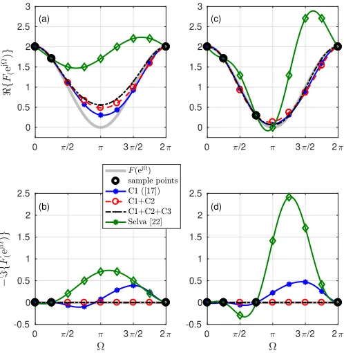
Fig. 4. Smooth approximations of F(ejΩ_{) using various interpolation}

approaches given (a,b)K= 2and (c,d)K= 3sample points.

with B1 ∈ RL×L and all other components of appropriate dimensions. Based on the solution to

minx[F(q),T xT_]B[F(q),T

xT_]T_{, the smoothness metric}

for the optimal completionx is given by [20]

χmin=F(q),T(B1−B2B−41B T 2)F

(q)

via the Schur complementB1−B2B−41BT2 of B, but which

differently from [20] incorporates the additional constraints.

VII. RESULTS ANDDISCUSSION

We first provide an example for the interpolations achieved by various settings, benchmarked against [20] and [21], whereby the latter aims to achieve a time domain response that does not exceed a support of K, without explicit de-sire for smoothness but at minimal computational cost. In Fig. 4, we see a sampling grid of N = 8 for the function

F(ejΩ_{) = 1 + cos Ω, and are given (i) K = 2 sample points}

fork={0,1}and (ii)K= 3sample points fork={0,1,3}. As the number of sample points increases, the interpolated function is further tied down and therefore better approximates the original F(ejΩ_{). A similar effect can be observed as}

more constraints are taken on board. Constraining the missing sample points to be real valued provides a small enhancement and eliminates any deviation in the imaginary part, while the symmetry condition essentially increases the number of given sample points.

When checking on the Pth derivative power σ_P2 of an interpolation based on K given sample points of the above

F(ejΩ_{), the metrics in Tab. I for P = 5 are returned.}

Note that as K and the number of constraints increases, the values converge towards the true σ2

P =

1

TABLE I

POWER IN THEP= 4TH DERIVATIVE OF AN INTERPOLATION DRIVEN BY A COST FUNCTION WITHP= 4FOR A VARIABLE NUMBERKOF SAMPLE

POINTS ON A GRIDN= 8.

K C1 [20] C1+C2 C1+C2+C3 Selva [21] 2 0.152832 0.196791 0.401503 0.146447 3 0.438293 0.445379 0.488754 5.707107 4 0.493379 0.493481 0.499909 51.935029 5 0.499571 0.499572 0.500000 297.524387 6 0.499368 0.499368 0.500000 761.419354 7 0.499929 0.499929 0.500000 333.250000 8 0.500000 0.500000 0.500000 0.500000

Selva [21], which aims to solve the missing samples problem by providing an interpolation for a compactf[τ]◦—•F(ejΩ₎

via a highly efficient fast Fourier transform scheme, does not offer the smooth interpolation that we seek.

Without the additional constraints C1–C3, in [20] the constraint optimisation was found to have lower complexity and better conditioning compared to the Schur approach for

K N, and vice versa for K → N. Here, with additional constraints, the cost is shifted: MVDR is computationally more expensive due to the increased dimension of the constraint matrix, while the Schur complement scheme — dominated the matrix inverse ofB4 — contents with a lower dimension

and therefore lower cost.

VIII. CONCLUSIONS

This paper has illuminated properties of a cost function that evaluates the power of derivatives from the smoothest possible interpolation through a potentially incomplete number of sample points on the unit circle. The particular type of function to be interpolated here are eigenvalues, which in the Fourier domain will be non-negative, real-valued, and can potentially be symmetric. The cost function can be evaluated as a weighted inner product of the coefficient vector, whereby the weighting matrix is real-valued and circulant.

The real-valuedness and potential symmetry of eigenvalues can be enforced by constraints, which also aids in matching the power of the derivatives of an approximated function more closely. We have benchmarked this method against the previously existing approach in [20], and compared it to a low-cost interpolation in [21]. The latter is not aimed at providing a maximally smooth interpolation but sets an aspiration in terms of its very low computational footprint.

Therefore, the proposed metric offers some good properties for the extraction of analytic factors for, for example, the EVD of an analytic, parahermitian matrix [12], [13]. Analyticity in turn offers the opportunity of Laurent polynomial approxima-tions that can be siginificantly lower in order than for factors that are obtained by current time domain algorithms favouring spectral majorisation [4], [5], [7], [9]. With lower order poly-nomials translating into lower implementation cost, the pro-posed metric may directly contribute to reduced computational cost for applications such as broadband beamforming [24], angle or arrival estimation [25], or source separation [26].

REFERENCES

[1] P. P. Vaidyanathan,Multirate Systems and Filter Banks, Prentice Hall, Englewood Cliffs, 1993.

[2] S. Weiss, J. Pestana, and I.K. Proudler, “On the existence and uniqueness of the eigenvalue decomposition of a parahermitian matrix,”IEEE TSP,

66(10):2659–2672, May 2018.

[3] S. Weiss, J. Pestana, I.K. Proudler, and F.K. Coutts, “Corrections to ‘On the existence and uniqueness of the eigenvalue decomposition of a parahermitian matrix’,” IEEE TSP,66(23):6325–6327, Dec. 2018. [4] J.G. McWhirter, P.D. Baxter, T. Cooper, S. Redif, and J. Foster,

“An EVD Algorithm for Para-Hermitian Polynomial Matrices,” IEEE Trans. SP,55(5):2158–2169, May 2007.

[5] S. Redif, J.G. McWhirter, and S. Weiss, “Design of FIR paraunitary filter banks for subband coding using a polynomial eigenvalue decom-position,” IEEE Trans. SP,59(11):5253–5264, Nov. 2011.

[6] J. Corr, K. Thompson, S. Weiss, J.G. McWhirter, S. Redif, and I.K. Proudler, “Multiple shift maximum element sequential matrix diagonalisation for parahermitian matrices,” inIEEE SSP, Gold Coast, Australia, June 2014, pp. 312–315.

[7] S. Redif, S. Weiss, and J.G. McWhirter, “Sequential matrix diagonaliza-tion algorithms for polynomial EVD of parahermitian matrices,” IEEE Trans. SP,63(1):81–89, Jan. 2015.

[8] Z. Wang, J. G. McWhirter, J. Corr, and S. Weiss, “Multiple shift second order sequential best rotation algorithm for polynomial matrix EVD,” in

EUSIPCO, Nice, France, Sep. 2015, pp. 844–848.

[9] J.G. McWhirter and Z. Wang, “A novel insight to the SBR2 algorithm for diagonalising para-hermitian matrices,” in IMA Maths in Signal Proc., Birmingham, UK, Dec. 2016.

[10] M. Tohidian, H. Amindavar, and A.M. Reza, “A DFT-based approximate eigenvalue and singular value decomposition of polynomial matrices,”

J. Adv. SP,2013(1):1–16, 2013.

[11] F.K. Coutts, K. Thompson, S. Weiss, and I.K. Proudler, “A comparison of iterative and DFT-based polynomial matrix eigenvalue decomposi-tions,” inIEEE CAMSAP, Curacao, Dec. 2017.

[12] F.K. Coutts, K. Thompson, J. Pestana, I.K. Proudler, S. Weiss, “En-forcing eigenvector smoothness for a compact DFT-based polynomial eigenvalue decomposition,” inIEEE SAM, Sheffield, UK, July 2018. [13] S. Weiss, I.K. Proudler, F.K. Coutts, and J. Pestana, “Iterative

approxi-mation of analytic eigenvalues of a parahermitian matrix EVD,” inIEEE ICASSP, Brighton, UK, May 2019.

[14] B.L.R. De Moor and S.P. Boyd, “Analytic properties of singular values and vectors,” Tech. Rep., KU Leuven, 1989.

[15] A. Bunse-Gerstner, R. Byers, V. Mehrmann, and N.K. Nicols, “Numeri-cal computation of an analytic singular value decomposition of a matrix valued function,” Numer. Math.,60:1–40, 1991.

[16] K. Wright, “Differential equations for the analytic singular value decomposition of a matrix,” Numer. Math.,63(1):283–295, Dec. 1992. [17] L. Dieci and T. Eirola, “On smooth decompositions of matrices,”SIAM

J. Matrix Analysis and Applications,20(3):800–819, 1999.

[18] E.S. Van Vleck,Numerical algebra, matrix theory, differential-algebraic equations and control theory, chapter Continuous Matrix Factorizations, pp. 299–318, Springer, 2015.

[19] F. Rellich, “St¨orungstheorie der Spektralzerlegung. I. Mitteilung. An-alytische St¨orung der isolierten Punkteigenwerte eines beschr¨ankten Operators,”Math. Annalen,113:DC–DCXIX, 1937.

[20] S. Weiss and M.D. Macleod, “Maximally smooth Dirichlet interpolation from complete and incomplete sample points on the unit circle,” inIEEE ICASSP, Brighton, UK, May 2019.

[21] J. Selva, “FFT interpolation from nonuniform samples lying in a regular grid,” IEEE TSP,63(11):2826–2834, June 2015.

[22] G.H. Golub and C.F. Van Loan, Matrix Computations, John Hopkins University Press, Baltimore, Maryland, 3rd edition, 1996.

[23] R.G. Lorenz and S.P. Boyd, “Robust minimum variance beamforming,”

IEEE TSP,53(5):1684–1696, May 2005.

[24] S. Weiss, S. Bendoukha, A. Alzin, F.K. Coutts, I.K. Proudler, and J.A. Chambers, “MVDR broadband beamforming using polynomial matrix techniques,” inEUSIPCO, Nice, Sep. 2015, pp. 839–843. [25] M. Alrmah, S. Weiss, and S. Lambotharan, “An extension of the

MUSIC algorithm to broadband scenarios using polynomial eigenvalue decomposition,” inEUSIPCO, Barcelona, Aug. 2011, pp. 629–633. [26] S. Redif, S. Weiss, and J.G. McWhirter, “Relevance of polynomial

matrix decompositions to broadband blind signal separation,”Sig. Proc.,